Evaluating Sampling Strategies for Characterizing Energy Demand in Regions of Colombia Without AMI Infrastructure

Abstract

This study presents and evaluates three sampling strategies to characterize electricity demand in regions of Colombia with limited metering infrastructure. These areas lack Advanced Metering Infrastructure (AMI), relying instead on traditional monthly consumption records. The objective of the research is to obtain user samples that are representative of the original population and logistically efficient, in order to support energy planning and decision-making. The analysis draws on five years of historical data from 2020 to 2024. It includes monthly energy consumption, geographic coordinates, customer classification, and population type, covering over 500,000 users across four subregions of operation determined by the region grid operator: North, South, Center, and East. The proposed methodologies are based on Shannon entropy, consumption-based probabilistic sampling, and Kullback–Leibler divergence minimization. Each method is assessed for its ability to capture demand variability, ensure representativeness, and optimize field deployment. Representativeness is evaluated by comparing the differences in class proportions between the sample and the original population, complemented by the Pearson correlation coefficient between their distributions. Results indicate that entropy-based sampling excels in logistical simplicity and preserves categorical diversity, while KL divergence offers the best statistical fit to population characteristics. The findings demonstrate how combining information theory and statistical optimization enables flexible, scalable sampling solutions for demand characterization in under-instrumented electricity grids.

1. Introduction

1.1. Background and Motivation

Accurate characterization of electricity demand is fundamental for planning and managing power systems. In regions with advanced metering infrastructure (AMI), this process can rely on granular, real-time data collected through smart meters. However, in many developing regions, especially in Latin America, AMI deployment remains extremely limited. In Colombia, for example, fewer than 4% of users were equipped with smart meters as of 2021, despite a national goal of 75% coverage by 2030 [1]. This lack of granular, high-frequency data restricts the implementation of demand-side management, real-time control, and efficient forecasting. As a result, utilities in these regions must rely on alternative approaches to understand user behavior and support energy planning, using conventional metering infrastructure based on monthly or manual readings [2].

Conventional metering methods suffer from several key limitations. Monthly consumption records provide only a coarse summary of usage and fail to capture temporal patterns like peak hours or daily variability. These gaps introduce uncertainty into load forecasting, tariff design, and infrastructure investment decisions [3]. Moreover, the low resolution of conventional data prevents the application of advanced strategies like time-of-use pricing or grid-responsive load management. Existing methods for characterizing electricity demand largely rely on data from smart metering infrastructure. However, in many developing regions, this technology is unavailable. There is a need for scalable, low-cost sampling strategies that can provide representative insights without relying on AMI.

1.2. Low Infrastructure Development in the Colombian Context

The need for alternative demand characterization strategies is especially relevant in regions with low infrastructure development. This term refers to areas with poor grid coverage, unreliable service, minimal digital infrastructure, and—of special interest to this research—limited access to modern metering technologies. In Colombia, such conditions are found in the rural and mountainous areas of the Andean region, where economic and topographical barriers hinder electrification. High installation costs, difficult terrain, and low customer density make it economically unattractive to extend infrastructure [4]. Studies estimate that in these areas, logistics and transport alone can account for over 50% of the cost of electrification projects [5]. Despite national electrification rates above 97%, these underserved zones face persistent energy insecurity—some communities receive less than four hours of electricity per day or remain entirely off-grid [6].

1.3. Research Objectives and Hypothesis

A flexible and low-cost strategy is useful in addressing the challenges presented by the low-tech areas found in this region of Colombia [7]. To address these challenges, this paper proposes and evaluates three sampling methodologies designed to characterize energy demand in regions without AMI. Each methodology is built on a distinct theoretical foundation—information theory, statistical modeling, and probabilistic optimization—and is adapted to work with the type of conventional data typically available to utilities in developing countries. These techniques allow the present use case to be studied from complementary approaches uncommon in the state of the art. The goal is to select statistically representative user samples that enable accurate energy planning while remaining logistically feasible in difficult environments. The proposed strategies are tested using real-world data from a Colombian grid operator covering four subregions in the central Andean area.

This study seeks to answer how energy demand can be effectively characterized in regions with low infrastructure development and without AMI, using only conventional metering data. In pursuit of this objective, the paper develops and applies three sampling strategies tailored to data-scarce contexts, compares the effectiveness of each method in terms of statistical representativeness and logistical feasibility, evaluates trade-offs between categorical diversity, consumption coverage, and spatial distribution, and recommends sampling strategies appropriate for different planning needs in infrastructure-limited environments. The working hypothesis guiding this study is that it is possible to construct statistically representative and operationally viable energy demand samples in low-infrastructure regions using conventional metering data through the integration of entropy-based, consumption-based, and divergence-minimizing sampling strategies. This addresses the need for more efficient approaches to energy management in developing regions.

1.4. Structure of the Paper

The remainder of this paper is organized as follows. Section 2 presents a detailed review of existing sampling approaches and demand characterization techniques, particularly in AMI-scarce contexts. Section 3 describes the mathematical foundations behind each sampling strategy, including entropy, probabilistic sampling, and KL divergence. Section 4 explains the data sources, preprocessing steps, regional context, and implementation of the sampling methodologies. Section 5 presents results of the strategies based on statistical fit, spatial distribution, and category coverage. Section 6 presents a discussion of the results, evaluating the applicability and limitations of each approach in the context of developing regions. Section 7 concludes the paper by summarizing key findings, outlining policy and operational recommendations, and suggesting directions for future research.

2. Literature Review

The characterization of energy demand in regions lacking Advanced Metering Infrastructure (AMI) presents a unique set of challenges. Most conventional approaches to demand estimation rely on granular, high-frequency data that AMI systems provide. However, in much of Latin America, and especially in Colombia, these technologies remain under-deployed due to a combination of economic, technical, and regulatory factors [3,4,6]. Technically, AMI systems require robust and reliable communication infrastructure, which is often lacking or unreliable in rural and mountainous areas of Colombia, particularly in the Andean region. These areas also face significant logistical barriers to installation and maintenance. From a regulatory standpoint, delays in standardization, limited incentives for private utilities to invest in metering upgrades, and insufficient funding programs have all slowed AMI adoption [3,4,6]. Therefore, alternative methods capable of functioning under low-data conditions are needed for effective planning and demand management.

This review is structured into three main thematic groups. (i) Machine-learning-based and AMI hybrid modeling techniques for demand estimation with limited data, which are the most common type of techniques found in the recent literature. (ii) Statistical and stratified sampling strategies used in demand characterization. (iii) Emerging information-theoretic approaches, including the use of entropy and Kullback–Leibler divergence for sample optimization. These last two points are more closely related to the purposes of this study. Each group is examined with an emphasis on its applicability to low-infrastructure contexts, and its relevance to the proposed methodologies in this study.

2.1. Demand Modeling with ML and Hybrid Approaches

Traditionally, demand estimation in regions with limited data availability has been addressed through mathematical modeling techniques. Early efforts used Monte Carlo simulations to estimate residential transformer loads, aiding in grid expansion planning [1]. These models function by using probabilistic reconstructions of load curves from aggregated or infrequent data. Monte Carlo methods align with the goals of this study in that they enable the composition of a user sample by extracting users from a reconstructed demand curve. However, unlike the proposed information-theoretic strategies, Monte Carlo techniques are less efficient at identifying areas of high diversity for sampling and do not inherently optimize information gathering, as this method is random. It is possible to directly quantify uncertainty (via entropy) or divergence from population distributions (via KL divergence) to guide sampling placement.

As modeling techniques advanced, more sophisticated tools such as regression, clustering, and wavelet analysis were incorporated to improve accuracy and represent heterogeneity in consumption [8,9]. Furthermore, the concept of community networks has been applied to group curves and improves the detection of consumption patterns [10]. In a study on under-electrified rural regions, hierarchical clustering and geospatial proxies like satellite imagery were used to estimate demand [11]. This approach emphasizes the value of indirect indicators—a strategy that complements the use of entropy by validating the usefulness of external features for demand estimation.

The integration of AI and machine learning has enhanced these models, enabling more dynamic representations of consumption patterns. For example, clustering methods have been used to disaggregate aggregated loads, while LSTM neural networks and nonparametric regression have been applied to adaptively predict variations linked to new technologies like electric vehicles or solar PV [12,13]. Bayesian inference has also been used to reconstruct consumption from readings in low-income regions [14]. Despite their promise, these methods are often constrained by the need for large training datasets, which are not so often available in low-infrastructure regions [1].

Hybrid models that leverage limited smart meter data have also been developed. Hybrid models that combine statistics and machine learning have been proposed to improve demand prediction. One approach integrates MEMD with PSO-optimized SVR and improves the estimation of daily peaks [15]. Another model combines IEMD, ARIMA, and FOA-optimized Wavelet Neural Networks to predict short-term load [16]. A strategy combining SVR with fuzzy systems has been proposed. This approach improves the management of nonlinear weather conditions and reduces load uncertainty. This increases the accuracy of daily forecasting [17]. These methodologies allow for the inference of detailed consumption patterns and improve energy management in regions where the AMI infrastructure does not have complete coverage. To characterize demand in systems without full AMI coverage, hybrid models that combine limited data with machine learning have been developed. One study combined ARIMA, logistic regression, and neural networks to predict peak load days. This facilitates demand response and reduces costs [18]. Additionally, an intelligent system was designed to manage non-technical losses in residential users. This system uses machine learning to detect anomalies [19]. Load disaggregation models are applied in smart buildings that allow the identification of the consumption of each device [20]. Nevertheless, while effective, these methods still depend on at least partial AMI coverage and significant computational resources.

2.2. Stratified and Statistical Sampling in Demand Estimation

Given the limitations of modeling techniques in data-scarce environments, statistical sampling strategies are a practical alternative. Sampling allows for the collection of data from a representative subset of users, reducing monitoring costs while still providing valid inferences about the broader population [21].

An effective technique for representing different types of users is stratified sampling. This method divides the population into homogeneous subgroups based on criteria such as user type, location, or consumption level. This improves the accuracy of inferences and reduces bias. For example, the TURKSTAT 2019 Household Budget Survey applied stratified cluster sampling to estimate monthly electricity consumption in households in Turkey. This improved the extrapolation of results [22]. In Colombia, similar approaches have been employed by public utilities to improve the representativeness of manual metering surveys [5]. Sample size determination in these methods typically relies on Cochran’s formula, accounting for desired confidence levels and margins of error. Some studies have also recommended post-survey validation through follow-up interviews or statistical comparisons with known consumption distributions [23]. Although effective, stratified sampling methods often lack the mathematical rigor to optimize sampling placement, especially in heterogeneous regions.

To overcome this, smart sampling techniques have been introduced. These approaches utilize clustering algorithms, historical billing data, and optimization metrics to select the most informative users or time periods for measurement. One example is machine-learning-assisted active sampling, which alternates between estimation and data collection based on predictions about unobserved data [24]. In environmental monitoring, a strategy for selecting sampling sites for micropollutants in rivers is proposed that combines spline interpolation, hierarchical analysis, and geographic information systems to optimize spatial distribution [25]. In fields like deep metric learning, an approach based on clustering representations in feature spaces has been proposed to select informative samples. This improves convergence by avoiding local minima [26]. Sampling is also essential in contexts with unbalanced data. Increasing the sample size and balancing classes improves accuracy and predictive power. The choice of random seeds also influences the stability and generalization of the model [27]. Furthermore, Gibbs sampling in conjunction with GRNN neural networks allows the generation of synthetic samples that preserve the original structure of the data. This improves the representation of the true distribution and the predictive performance in contexts with limited data [28]. These advances show the variety of methodologies and highlight the importance of adapting each technique to its context. However, once again, these methods are limited by the availability of data in regions with limited measurement infrastructure. Deep-learning-based methods generally improve as the amount of data increases. They often outperform other techniques when trained on very large datasets, magnitudes greater than a million records [29]. Time-series scenario reduction through smart sampling has been used to maintain accuracy in power flow simulations while lowering computational loads [30]. Algorithms like A-DPC apply sampling logic to allow prioritizing customers in response programs based on their consumption patterns. This increases the effectiveness of the strategies [31]. In informal settlements in Kenya, combining stratified sampling with regression has improved consumption estimation [32]. Demand characterization has improved thanks to data-driven load modeling too. These techniques capture the diversity and variability of loads in distribution networks and improve simulation and planning [33]. However, all these studies lack divergence-based optimization or the determinism and clarity of a fixed metric such as entropy proposed in this study.

2.3. Information-Theory Approaches to Sample Optimization

More recently, information-theoretic metrics have been introduced into sampling methodology to improve efficiency and representativeness. These approaches are particularly valuable in regions where AMI is absent and the sampling budget is constrained. Among these metrics are Shannon entropy and Kullback–Leibler (KL) divergence.

Entropy-based sampling identifies users or areas with high diversity in consumption, ensuring that the most informative data is collected [34]. In semi-rural grids, entropy-maximizing models have been used to reconstruct load curves using limited and coarse data sources [35]. Entropy-based selection has shown promise in identifying diverse consumption zones even when only billing or categorical data is available [34]. These studies support the strategy of targeting uncertainty-rich areas—a foundational principle in the methodology proposed in this study.

KL divergence, on the other hand, provides a quantitative measure of how one probability distribution diverges from another. In sampling, it can be used to select subsets whose aggregate consumption profile most closely resembles the full population, minimizing representational bias. This is particularly useful when comparing sample-generated distributions to known or estimated consumption patterns. When combined with clustering or smoothing techniques, KL divergence-based sampling has proven to yield robust results even in data-scarce settings [36,37].

Both entropy and KL divergence can complement stratified methods, adding quantitative rigor to group definitions and sample selection. The methods proposed in this study—Shannon Entropy Sampling and KL Divergence Sampling—build on these principles, offering flexible yet statistically grounded tools for representative sampling in low-infrastructure regions. These approaches directly address reviewer concerns about the lack of discussion comparing conventional techniques like stratified sampling to more sophisticated methods. While stratified sampling ensures group-level representation, entropy and divergence optimize for information content and distributional fidelity, respectively. The proposed methodology bridges these strategies, enhancing applicability to Colombia’s Andean region where infrastructure, terrain, and socioeconomics vary significantly.

3. Theoretical Framework

3.1. Shannon Entropy for Identifying High-Information Transformers

Shannon entropy is a measure of the uncertainty or amount of information contained in a random variable. In the context of energy sampling, it can be used to identify distribution transformers whose users provide the most information. For example, this occurs when there are more diverse demand patterns depending on the type or population of the user. The entropy of a discrete variable $X$ with probabilities $p_i$ for each possible state $x_i$ is calculated as [38]:

$$H\left(X\right)=-\sum _i{p}_i{log}_2\left(p_i\right)$$

(1)

3.2. Cochran’s Formula for Optimal Sample Size in Electricity Consumer Studies

This formula is used to calculate sample size for infinite populations under a specific confidence level and margin of error.

$$n_0={\displaystyle \frac{Z^2\cdot p\cdot (1-p)}{e^2}}$$

For a finite population $N$ the adjusted formula is:

$$n={\displaystyle \frac{n_0\cdot N}{n_0+N-1}}$$

(2)

The proportion p represents the expected fraction of the population with the characteristic of interest. For example, if it is known that 40% of the population uses renewable energy, $p$ = 0.4 can be used as the probability of selecting a user who consumes these energies. Without prior data, it is recommended to keep $p$ = 0.5 [39]. Section 5.1 of the results presents the sample size calculation for different confidence levels for each of the four subregions. The size of the original population for each subregion is also indicated. Z is the score for the selected confidence level and indicates the margin of error.

-

99% → 2.576

-

98% → 2.326

-

95% → 1.96

-

90% → 1.645

3.3. Logarithmic Discretization to Represent Consumption Across Multiple Scales

Logarithmic discretization transforms continuous values by grouping them into increasing intervals according to a logarithmic scale. Linear discretization uses equidistant intervals. However, logarithmic discretization uses exponentially increasing limits. It is useful for data that cover several orders of magnitude. For example, energy consumption data includes users with very low and very high consumption. This approach allows for the use of more precise intervals for small values and wider intervals for large values. It better represents variability and prevents high consumption from being under-represented. For a continuous data set $X$ divided into $B$ intervals:

$$b_i=exp\left(log\left(x_{min}\right)+i{\displaystyle \frac{log\left(x_{max}\right)-log\left(x_{min}\right)}{B}}\right)$$

(3)

For $i=1,2,\dots B$, where $b_i$ is the upper bound of the interval. Logarithmic scaling is applied by calculating the logarithm of the minimum and maximum values. The values are then divided into $B$ equidistant intervals in the logarithmic space. Finally, the inverse exponential is applied to return to the original scale and the exponentially growing bounds are obtained. This allows the data to be grouped proportionally to its scale instead of using fixed intervals [40]. In this study, logarithmic discretization was applied to the monthly consumption data of 502,347 electricity users across four Colombian subregions. The minimum recorded monthly average consumption was 5 kWh and the maximum exceeded ${10}^6$ kWh. Using $B=90$, the logarithmic transformation ensured that the lower-consumption users (around less than 100 kWh/month, typically rural or low-income households) were captured, just like higher-consumption users (superior to ${10}^4$ kWh/month, often commercial or industrial users). This prevented under-representation of small-demand and high-demand users, capturing the tail behavior of the demand curve.

3.4. Smoothing Functions to Improve Representation of Rare Consumption Patterns

This method seeks to give a higher probability to less frequent elements without significantly altering the original distribution. To do this, a parameter β is introduced that regulates the degree of smoothing [41]. The distribution is normalized by dividing each value by the total sum. Then, the average of the normalized distribution is calculated. Finally, values greater than the average are slightly reduced and those lower than the average are increased, increasing the probability of the less common ones. This function is applied to each $x_i$ of the distribution:

$${x’}_i=x_i-\beta \left(x_i-\mu \right)$$

(4)

$\mu$ is the mean of the normalized distribution and $\beta$ is the smoothing factor with values between 0 and 1. If $\beta <0$, the term $-\beta \left(x_i-\mu \right)$ changes sign, so instead of pulling values towards the mean $\mu$, it pushes them away from it. That means frequent elements get even more dominant and rare elements get even rarer—exactly the opposite of the smoothing goal. This would exacerbate inequality in the distribution. If $\beta >1$, the adjustment overshoots the mean, excessively distorting the distribution. It follows that if $\beta =0$, then ${x’}_i=x_i$, and if $\beta =1$, all values converge to ${x’}_i=\mu$. Therefore constraining $\beta$ to the interval [0, 1] ensure the transformation is a weighted average between $x_i$ and $\mu$, so each value is moved closer to the mean, proportionally to $\beta$, without crossing it. This ensures a controlled and predictable smoothing effect.

3.5. Kullback–Leibler Divergence as a Statistical Similarity Measure for Sampling

It is a measure of the difference between two probability distributions. It is based on cross entropy, which represents the degree of uncertainty that would arise when using a $q\left(x\right)$ distribution instead of a reference $p\left(x\right)$ distribution to describe a set of events [42]. The KL divergence is defined as [43]:

$$DKL\left(p\right|\left|q\right)=H(p,q)-H\left(p\right)$$

(5)

where $H(p,q)$ is the cross entropy and $H\left(p\right)$ is the entropy for the distribution $p\left(x\right)$ that measures the uncertainty of $p\left(x\right)$. The KL divergence measures the difference between both, that is, how much additional information is needed when using $q\left(x\right)$ instead of $p\left(x\right)$. If $q\left(x\right)=p\left(x\right)$ then $H(p,q)=H\left(p\right)$ and the divergence is minimal with $DKL\left(p\right|\left|q\right)=0$. As the divergence increases, more additional information is required to get from $q$ to $p$. This is because there is greater loss of information and there is greater difference between both distributions. In this context, KL divergence was selected over other statistical divergence measures—such as Jensen–Shannon divergence or total variation distance—because it directly quantifies the loss of information when a sample distribution is used to approximate the full population distribution. This aligns with one of the goals of the proposed methodology: to ensure that the sampled subset retains the maximum possible fidelity to the original population in terms of categorical and consumption distributions. Additionally, KL divergence has an intuitive interpretation: a value of zero represents the ideal case of perfect representativeness, making it easier to compare and interpret results across different sampling strategies. Moreover, its interpretation and compatibility with entropy-based methods make it a natural complement to the Shannon entropy strategy, allowing both techniques to share a common information-theoretic foundation.

4. Materials and Methods

The present study aims to develop and evaluate three sampling strategies for characterizing electricity demand in regions of Colombia with limited metering infrastructure. The analysis is based on consumption and geospatial data provided by the regional electricity distribution company operating in the Andean area of Colombia.

4.1. Materials

4.1.1. Data Sources

The primary dataset consists of monthly electricity consumption records for all active users in the service area over a period of 58 consecutive months, from January 2020 to October 2024. Each record contains the following:

• User identifier (anonymized).
• Monthly energy consumption in kilowatt-hours (kWh).
• Transformer ID supplying the user.
• Customer type, classified as street lighting, commercial, industrial, official, provisional, residential (strata 1–6), and other.
• Population type, categorized as urban, rural, or populated center.
• Geographic coordinates (latitude and longitude) of the service point.

The geographic coordinates (latitude and longitude) of each user are available. Transformers—and, by extension, users—are classified into four subregions defined by the grid operator: North/Northwest, South/Southwest, Central, and East. This division allows the sampling problem to be broken down into four independent subproblems. Each sampling strategy can be applied separately in each subregion to achieve a more geographically representative sample. The North/Northwest subregion is primarily rural, with mountainous terrain and limited road infrastructure. The South/Southwest subregion combines growing rural and urban areas, with industrial and port activity concentrated near a major river. The Central subregion concentrates the main metropolitan areas and most of the population, with a variety of residential, commercial, and industrial users. The Eastern subregion has low elevations and a commercially important river. In general, temperate and warm thermal floors predominate throughout the region.

A total of 568,291 active users were identified, distributed across 20,102 transformers. In addition, a geographic assignment file for transformers was maintained. This file locates each transformer in one of the subregions of the company’s area of influence. The North/Northwest subregion has 117,399 users. The South/Southwest subregion has 169,165 users. The Central subregion has 213,260 users, and the East subregion has 68,468 users.

4.1.2. Data Processing and Preparation

Once the information sources were identified, the data were processed. An additional column was calculated with the average annual consumption in kWh. To do this, the monthly consumption for each year was added together to obtain the annual average. This measure summarizes user consumption and allows for the consideration of users who have missing records in some months. The annual average consumption represents the population’s consumption distribution. This distribution will be used as a basis for applying the sampling strategies. Each user has an associated transformer, and each transformer is classified into one of the four subregions. Users were then grouped into four subsets, and the sampling methodologies will be applied independently to each subset.

The result was a structured dataset of active users in the region. This dataset contains sufficient and reliable energy consumption information for appropriate sample selection.

4.2. Methods

4.2.1. Research Outline

This study aims to design, implement, and evaluate three distinct sampling strategies for characterizing electricity demand in regions of Colombia without Advanced Metering Infrastructure (AMI). The purpose is to develop cost-effective and logistically feasible approaches that preserve statistical representativeness despite the limitations of conventional metering systems.

The first stage consists of data acquisition and preprocessing. It is important to compile and prepare the necessary datasets to enable accurate and reliable sampling. Monthly consumption records, user classifications, and geographic information from the utility’s databases are compiled, cleaned, and standardized. The main goal is to obtain four consistent and comprehensive datasets for subsequent analysis, one for each subregion.

The second stage consists of the definition of sampling parameters. It is necessary to define appropriate parameters to manage a fixed and defined comparison framework between the different sampling approaches. The sample sizes for each subregion will be determined using Cochran’s formula, specifying the confidence level, and margin of error.

The third stage involves the development and application of sampling strategies. Three methodologies are tested: (i) Shannon entropy-based sampling, prioritizing categorical diversity; (ii) consumption-based sampling, emphasizing balanced coverage of different demand levels; and (iii) KL divergence-based sampling, integrating categorical and consumption representativeness through statistical optimization. From this stage, a sample of users is obtained for each of the three proposed methods.

The fourth stage focuses on evaluation and comparison, where it is assessed how well each method captures the characteristics of the full population while considering logistical efficiency. The performance of each strategy is assessed mainly using differences in category proportion and correlation coefficient. Spatial distribution of selected users is also examined to ensure geographical representativeness. The results of this evaluation will be reflected in Section 5 of results.

Finally, the fifth stage is based on integration and recommendation. The purpose is to identify the most suitable sampling strategies for various planning scenarios in low-infrastructure environments. Which results are synthesized to determine the most suitable strategies for different operational contexts in low-infrastructure regions. The conclusions drawn from this process are intended to guide utilities and policymakers in the design of sampling frameworks that can support energy planning in similar environments.

4.2.2. Sampling by Shannon Entropy Methodology

The sampling methodology based on Shannon entropy is presented. It aims to identify the transformers that provide the most information. The population connected to each transformer is analyzed according to its characteristics, and entropy is calculated to prioritize those with the greatest variety of profiles.

The process begins with calculating Shannon entropy for each transformer based on the associated users. Customer type and population type categories are considered. For each transformer, the proportion of users per category is determined. These proportions are used as probabilities to calculate the entropy using Formula (1). A category with probability 0 does not contribute to the entropy. To prevent small but diverse transformers from having an inflated value, the entropy is normalized by multiplying it by the number of users. This allows prioritizing transformers that have both diversity and volume at the same time. This achieves a representative and efficient sampling without having to measure many small transformers unnecessarily. A user ranking based on entropy is then constructed. Entropies are calculated by customer type and population type. Both rankings are combined with an adjustable weighting scheme that balances the selection criteria. Greater weight is given to the customer type due to its greater diversity, but the inclusion of rural users is ensured. To achieve this, several customer type/population type weight combinations are tested: 100/0, 90/10, 80/20, 70/30, 50/50, 30/70, 20/80, 10/90, 0/100. To validate the best combination of weights, the sample of users associated with each weight combination is obtained, and the proportion of these samples is determined based on the type of customer and population. The total cumulative difference between the proportions of each category and the proportions of the original population is then found. The weights whose associated sample yields the smallest cumulative difference are selected.

Cochran’s Formula (2) is applied with several confidence levels $c$: 99%, 98%, 95%, 90% and errors $1-c$. This to define the optimal sample size. From the ranking, processors are selected in descending order, and their users are extracted until the determined size is reached. Due to the variability in users per processor, there may be a slight difference between the ideal size and the obtained one.

Each subpopulation is treated separately, and the four subsamples are integrated into a final sample of the entire region. The overall process is shown in Figure 1.

4.2.3. Sampling by Consumption Methodology

The sampling methodology based on annual energy consumption seeks to construct a representative sample that captures the variability in demand levels within a region. Unlike pure random sampling, this approach applies adjustments to improve the representation of rare categories, such as users with very high or very low consumption.

To achieve this, logarithmic discretization and distribution smoothing techniques are used. The starting point is the distribution of annual consumption in kWh for each user. A small adjustment of 0.1 is added to avoid problems with consumption equal to 0 when applying logarithmic discretization. This discretization (3) allows for better grouping of users because consumption varies across several orders of magnitude. A linear scale would concentrate most users in a few low intervals and leave those with high demand under-represented. This generates a biased sample. In contrast, the logarithmic scale creates more balanced categories. Smoothing (4) is also applied with an adjustment factor of $\beta$ = 0.05. This prevents excessive bias toward the most frequent values and favors the inclusion of users with atypical consumption patterns, such as industrial users or those in strata 5 and 6. This value allows for equitable representation without significantly distorting the original distribution, something that does occur with values greater than.

After defining the sample size (2), the Monte Carlo method is used to select users. The process calculates the cumulative probability of each consumption interval. A random number ($n$) between 0 and 1 is generated, and a user is randomly selected within the corresponding interval based on where that number falls. For example, if two intervals have cumulative probabilities of 0.1 and 0.3, and $n$ falls between 0 and 0.1, a user is chosen from the first interval. If 0.1 $<n\le$ 0.3, a user is chosen from the second interval. The results from each subregion are combined into a final sample. Figure 2 shows the general outline of the process.

4.2.4. Sampling by KL Divergence Methodology

This section describes a sampling strategy that combines elements of previous methodologies, aiming to construct a representative sample in terms of both consumption patterns and customer type composition (which is the most informative category).

The process begins with logarithmic discretization and smoothing of the consumption distribution, followed by Monte Carlo random sampling. Instead of using a single random seed, multiple samples associated with different seeds within a range of 0, …, $n$ are generated. For each seed, the statistical closeness between the obtained sample and the population is evaluated based on customer type. The sample whose distribution minimizes the KL divergence is selected. This hybrid approach mitigates the effects of chance in sample selection and improves the quality of the derived energy analyses. Logarithmic discretization (3) is applied to user consumption to adjust for extreme values in the distribution and make it more manageable. The smoothing function (4) with $\beta$ = 0.05 is then applied. After this, we move on to iterating over a range of seeds between 0 and 10,000. This considering that each iteration takes an average of 20.87 s to be executed in a machine with 6 CPU cores—Socket-AM4-3.90 GHz and 16 Gb of memory. This metric was found using the utility library tqdm of Python 3.12.

In each iteration, a sample is drawn from the population using the corresponding random seed using the Monte Carlo method. Up to this point, the procedure is similar to that of the consumption-based sampling strategy. The generated sample is now taken and the KL divergence (5) between the distribution by customer type in the sample and the distribution by customer type in the population is calculated. The resulting value is saved. This process is repeated for the entire range of seeds. The final sample selected will be the one with the lowest KL divergence. This ensures that the sample is representative of both consumption patterns and customer type distribution. Consumption representativeness is achieved with the smoothed random sampling approach. Representativeness by customer type is achieved with the KL divergence criterion. This process is applied in each subregion (totaling 40,000 iterations) and the results are combined to form the final sample. Figure 3 shows the general outline of the process.

In summary, the three sampling strategies presented offer complementary approaches. The entropy-based strategy prioritizes the categorical diversity of users. The consumption-based strategy seeks balanced coverage of different consumption levels. The strategy based in KL divergence integrates both aspects through statistical optimization based on similarity to the general population.

5. Results of Sampling Strategies

5.1. Determination of Sample Size Across Subregions

This brief section presents

Table 1. Theoretical sample size by subregion for different confidence levels.

Level	Center	North	South	East	Total
0.90	68	68	68	68	272
0.95	384	383	384	383	1534
0.98	3329	3288	3316	3223	13,156
0.99	15,394	14,540	15,112	13,358	58,404

with the results for the theoretical sample sizes using Cochran’s Formula (2) segregated by subregion.

Based on the results in Table 1, a 95% confidence level with a 5% error was selected. This level provides a moderate sample size. The sample size becomes too large for a higher confidence level. This defeats the initial purpose of achieving a convenient sample size.

5.2. Samples Geospatial Distribution Comparation

This section presents a description and comparison of the spatial distribution obtained with the three sampling approaches applied. The maps shown have been anonymized and are intended solely to illustrate and compare the location of the selected users with the rest of the population.

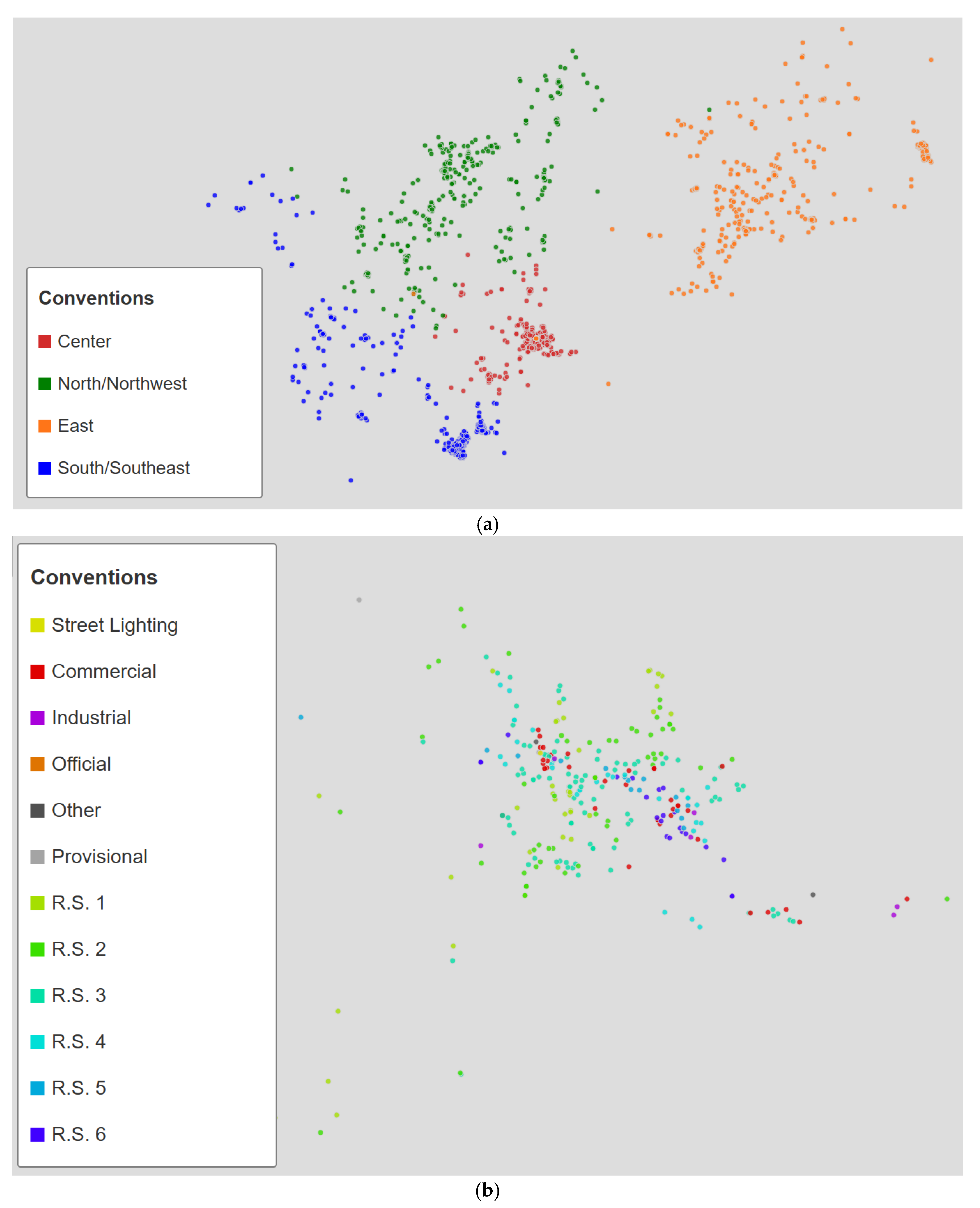
Figure 4 shows the spatial distribution of the sample based on Shannon entropy. This sample was obtained with a 95% confidence level and a customer/population weighting of 90/10 (the weighting is explained in Section 5.4). Figure 4b presents a close-up of a major city where a high concentration of users is observed in high-activity areas. Although there appear to be few selected users, they are actually so clustered that they are not clearly distinguishable on the overall map. To achieve a more uniform distribution, a 98% confidence level and a sample 7.7 times larger would be necessary. The clusters are located in residential neighborhoods of large cities where most consumption is concentrated. The clusters have so many residential users that commercial, official, and provisional users are not shown in this close-up of the city, and the street lighting points are covered by residential user points within the clusters. When analyzing each subregion, we also observe high-density areas near population centers. This reflects the natural pattern of consumption. This pattern is concentrated in a few urban centers. Figure 4a shows that dividing the problem by subregions disperses the concentrations more evenly throughout the region. This prevents the sample from concentrating in the central area, as would occur if sampling were applied directly to the entire population. This occurs because the transformers with the greatest diversity are in the largest cities.

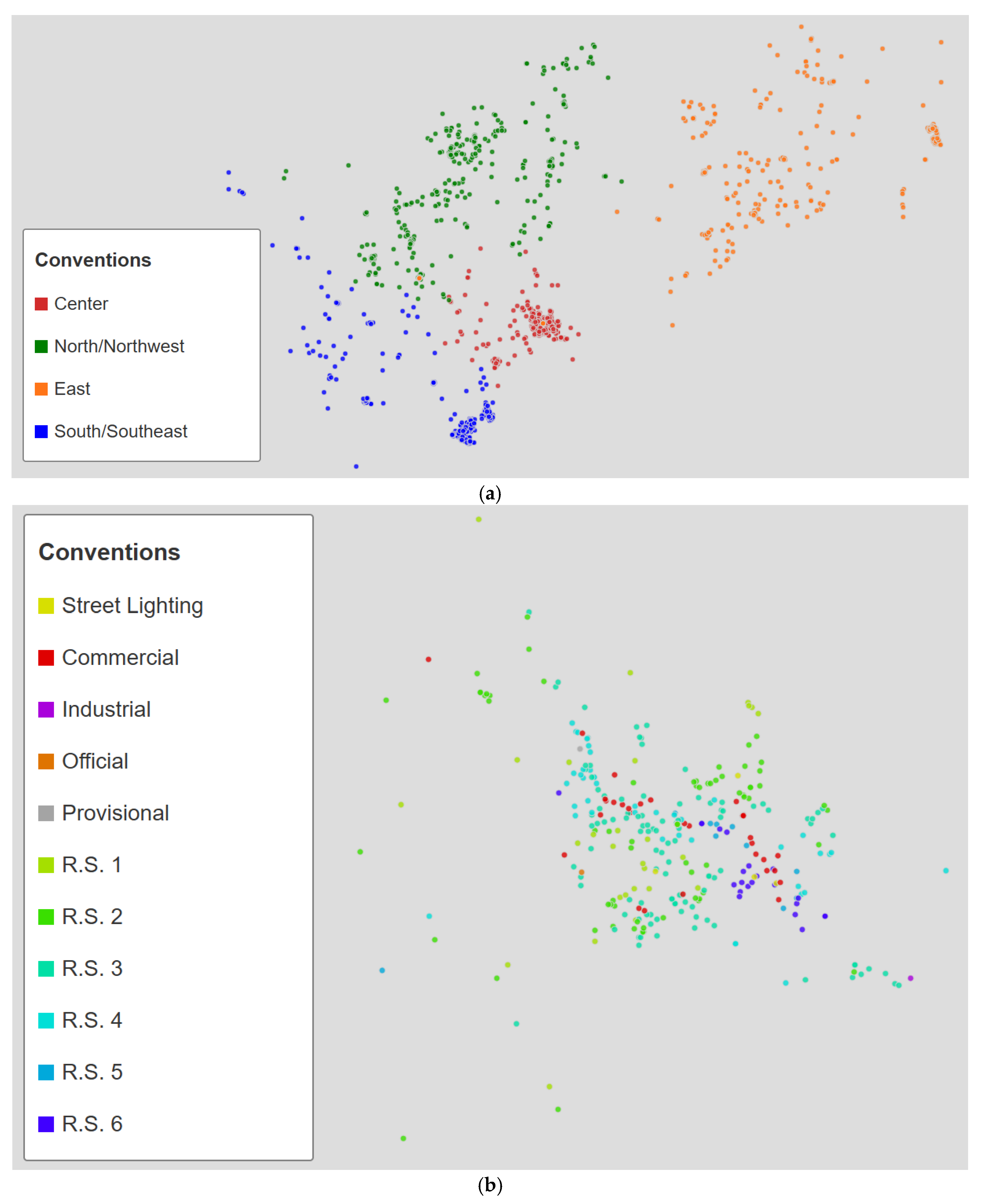
Figure 5 shows the spatial distributions of the consumption-based strategy. Figure 5a presents the general distribution across the entire region. Figure 5b shows a close-up of the same city used in Figure 4b. The main difference is greater geographic dispersion. Even within urban areas, dense clusters do not form, as is the case with entropy sampling. This occurs because the consumption-based strategy prioritizes diversity. Logarithmic discretization and smoothing are used to include users with atypical consumption patterns. While the entropy sample is concentrated in residential neighborhoods, the consumption sample has a greater presence of industrial users and users from strata 5 and 6 with high consumption. This is analyzed in Section 5.5.

Figure 6 shows the maps of the best sample according to the KL divergence criterion at 95% confidence level. Both Figure 6a,b show distributions very similar to that of the consumption sample. At first glance, it is not possible to adequately determine how the diversity of customer types in the KL divergence sample differs from the consumption sample. The difference between these two approaches will be better explored in the following consumption sample and KL Divergence results Section 5.4 and Section 5.5.

In summary, the spatial distribution maps clearly show the differences between the three strategies. The entropy sample tends to concentrate in densely populated areas and reflects the urban consumption pattern. The consumption sample shows greater geographic dispersion and seeks diversity by including atypical users. The KL divergence approach achieves a very similar geographic dispersion to that of the consumption sample. This may increase logistical complexity but improves overall coverage. This spatial comparison complements the analyses in subsequent sections and reinforces the importance of choosing a sampling strategy aligned with the operator’s objectives and the characteristics of the territory.

5.3. Evaluation and Results of the Sample by Shanon Entropy

This section presents the results of applying the Shannon entropy-based sampling strategy. The objective is to construct a sample that maximizes the amount of information contained in the selected users.

The first step was to select the weights between customer type and population type to construct the ranking of distribution transformers according to their entropy. For

Table 2. Difference between the proportions of the samples and those of the general population based on the categories according to the mixing proportion.

Differences in customer type proportions
	100	90	80	70	50	30	20	10	0
Total	13.5	44.7	35.2	34.9	51.5	60.6	60.6	65.8	76.5
Differences in population type proportions
Total	48.2	6.2	18.2	16.5	56.5	65.2	65.2	70.8	69.4
Acc.	61.7	50.9	53.3	51.4	108.0	125.8	125.8	136.6	145.9

The name of each column represents the weight for the customer type.

, samples with a 95% confidence level and different combinations of customer/population weights were generated. The proportions of each sample were then calculated by customer type and population type. These proportions were compared with those of the general population. Based on the differences, a cumulative total deviation was estimated, and the sample with the lowest deviation was selected. The best configuration was the 90/10.

The selected sample has 1750 users associated with eight distribution transformers (two transformers per subregion). These transformers have a normalized average Shannon entropy of 186.41. By comparison, the general population includes 569,423 users, 20,222 transformers, and their weighted average entropy with 90/10 weights is 12.03. The sample size for a 95% confidence level was determined to be 1525. However, the entropy strategy generates slightly different sizes. This is because transformers are selected to cover or exceed the theoretical size, and all users associated with each transformer are included to avoid losing information. Each transformer has a different number of users. Therefore, variations in size depend on the weighting, which affects the ranking of transformers.

Table 3. Difference in proportions between population and sample based on entropy by customer type and region.

Region	S.L.	Com.	Ind.	Off.	Oth.	Prov.	R.S.1	R.S.2	R.S.3	R.S.4	R.S.5	R.S.6
North	0.6	0.8	0.3	0.4	0.0	0.4	19.1	7.6	27.7	0.7	0.1	0.1
South	0.4	9.3	0.3	0.3	0.0	0.4	29.0	19.9	8.4	8.1	0.4	0.1
Center	0.7	6.9	0.3	0.3	0.0	0.4	46.5	8.3	24.9	11.6	4.0	6.4
East	0.6	6.9	0.1	1.0	0.0	0.4	7.0	11.9	9.5	0.8	0.2	0.1
General	0.6	1.6	0.3	0.3	0.0	0.0	20.2	2.1	8.6	7.0	1.7	2.4

S.L.: Street Lighting, Com.: Commercial, Ind.: Industrial, Off.: Official, Oth.: Other, Prov.: Provisional, R.S.: Residential Strata.

and

Table 4. Difference of average distances between users and population-sample ratios by population type and region for the entropy-based sample.

Region	P. Center	Rural	Urban	Avg. Distance [km]
North	18.32	26.72	45.04	06.04
South	3.41	20.00	23.41	6.78
Center	19.54	4.87	24.41	0.43
East	14.31	20.57	34.88	2.00
General	0.41	03.09	2.68	11.48

show the distribution of users by subregion with 95% confidence level and 90/10 weights, as well as the average distance between users. The Central subregion is the most urbanized subregion and has the smallest average distance from them all. Which is to be expected, since in an urban environment, users are closely located, living in residential neighborhoods that can group together several thousand people. This behavior is amplified within the entropy-based sample, since the sample tends to generate dense user clusters in these urban areas. To the point that the average distance in the central subregion is slightly smaller than the average distance for the entire population of this same subregion. The average distance between each user in the central subregion’s population is 7.41 km, while the average distance for the sample is 6.98 km, representing a difference of 0.43 km. On the other hand, the overall average distance of the whole sample increases by 11.48 km relative to the whole population. This is explained by the smaller number of users in the sample compared to the original total population, which will naturally make the sample more spatially sparse. The formation of clusters that leave gaps between subregions, especially in the mountainous Eastern subregion, will also be a normal cause that explains the increase in the average distance in the sample.

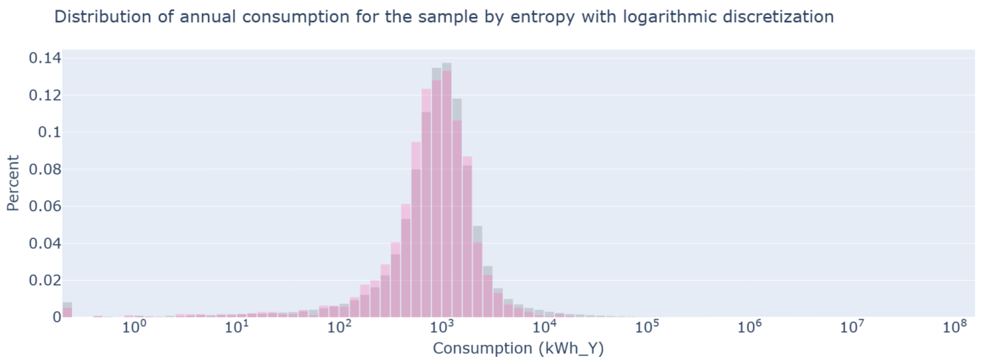
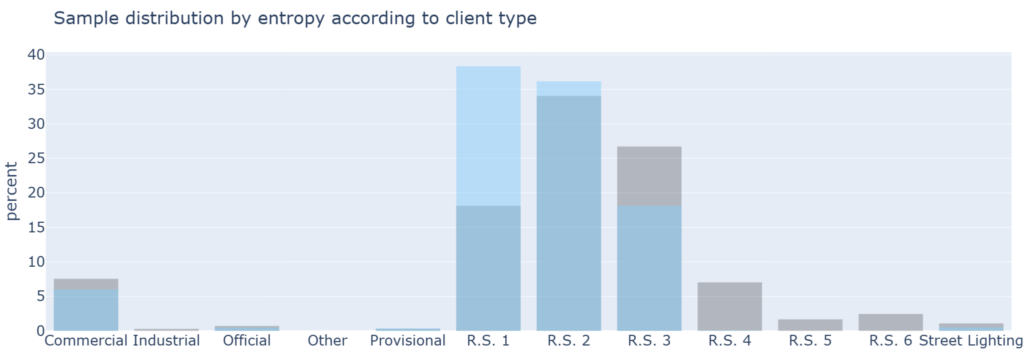
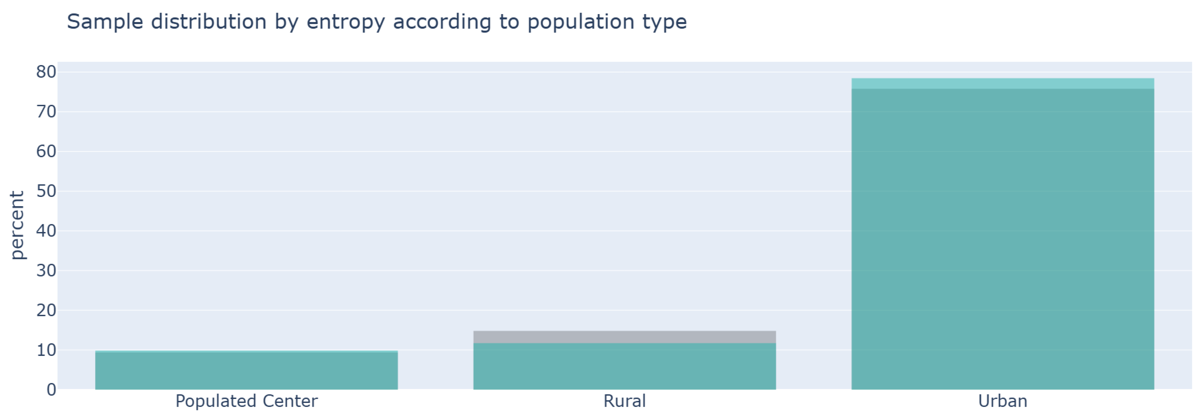
Figure 7 highlights an excellent fit with respect to annual consumption. This is achieved despite the fact that the sample is 325 times smaller than the population and does not use consumption as a selection criterion. This indicates that the customer type and population type categories contain relevant information about consumption patterns. This result is important because it shows that the sample can describe the demand of the original population. Figure 8 shows that the sample under-represents users in stratum 3 and does not include strata 4, 5, and 6. A bias that excludes high-income users is evident. A strong overrepresentation of users in stratum 1 is also observed. Correcting this bias would require increasing the confidence level. This would imply a significant increase in the sample size. Consumption-based and KL-divergence methodologies explore a consumption-based approach that seeks to alleviate this bias toward more atypical users. Figure 9 shows that the sample has a slightly lower proportion of rural users and a higher proportion of urban users. Even so, the overall fit for the population type category is good. This confirms that the 90/10 balance is adequate for this dimension.

Table 5. Pearson correlation coefficients and p-value for the entropy sample distributions with respect to the original population.

Distribution	Correlation	p-Value
Consumption	1	0
Customer Type	0.8768	0.0002
Population Type	0.9988	0.0316

provides the correlation coefficient values for the three sample distributions that were compared with those of the original population. The results for the consumption distribution are again noteworthy, with a coefficient of perfect 1. For the customer type and population distributions, values greater than 0.8 were obtained, reflecting moderately high representativeness. All distributions obtained a p-value less than 0.05, indicating significant relationships.

In summary, the entropy sampling strategy allows for the construction of samples with high informational diversity without using random sampling based on consumption as a direct criterion. Thanks to this, the approach provides deterministic results. Clusters are identified in densely populated areas. These excellently reflect the distribution of consumption and demand. The weighting between customer type and population makes it possible to maintain representativeness in key groups such as rural areas and low-income users. However, the sample tends to under-represent users with atypical consumption, such as industrial users or high-income users. Overall, it is a solid alternative for obtaining compact, information-rich, and logistically manageable samples.

5.4. Evaluation and Results of the Sample by Consumption

This section presents the results of applying the energy consumption-based sampling strategy. The objective is to construct a diverse sample that represents different consumption levels, highlighting less frequent patterns.

A 95% confidence level results in a sample of 1534 users.

Table 6. Difference in proportions between population and sample based on consumption by customer type and region.

Region	S.L.	Com.	Ind.	Off.	Oth.	Prov.	R.S.1	R.S.2	R.S.3	R.S.4	R.S.5	R.S.6
North	0.54	2.01	2.89	0.42	0.27	0.75	2.72	3.53	4.06	0.72	0.00	0.07
South	0.70	2.68	3.70	1.33	0.00	0.95	0.31	4.63	3.60	6.80	0.17	0.07
Center	0.53	1.87	02.06	0.26	0.52	0.16	2.20	1.60	3.37	2.29	1.07	0.56
East	0.56	1.14	0.65	0.61	0.52	1.07	4.65	2.99	3.08	0.53	0.03	0.13
General	0.05	2.00	2.30	0.87	0.33	0.71	5.48	0.17	7.78	2.86	0.28	0.98

S.L.: Street Lighting, Com.: Commercial, Ind.: Industrial, Off.: Official, Oth.: Other, Prov.: Provisional, R.S.: Residential Strata.

and

Table 7. Difference in average distances between users and population-sample ratios by population type and region for the sample based on consumption.

Region	P. Center	Rural	Urban	Avg. Distance [km]
North	4.72	0.83	5.55	0.68
South	5.70	1.78	7.49	3.90
Center	1.93	1.36	3.29	0.26
East	3.40	10.13	13.53	0.74
General	6.03	6.42	12.45	8.73

show the differences between the sample and the population by category and subregion. The differences are generally low, indicating a good fit and adequate representativeness. Table 6 uses the average distance between users as a measure of dispersion. This distance is greater than that of the original population in the North, South, and Central subregions. In the South subregion, the difference is 3.9 km. This confirms that the consumption sample is more dispersed. This dispersion ensures geographic coverage and representativeness even in small populations.

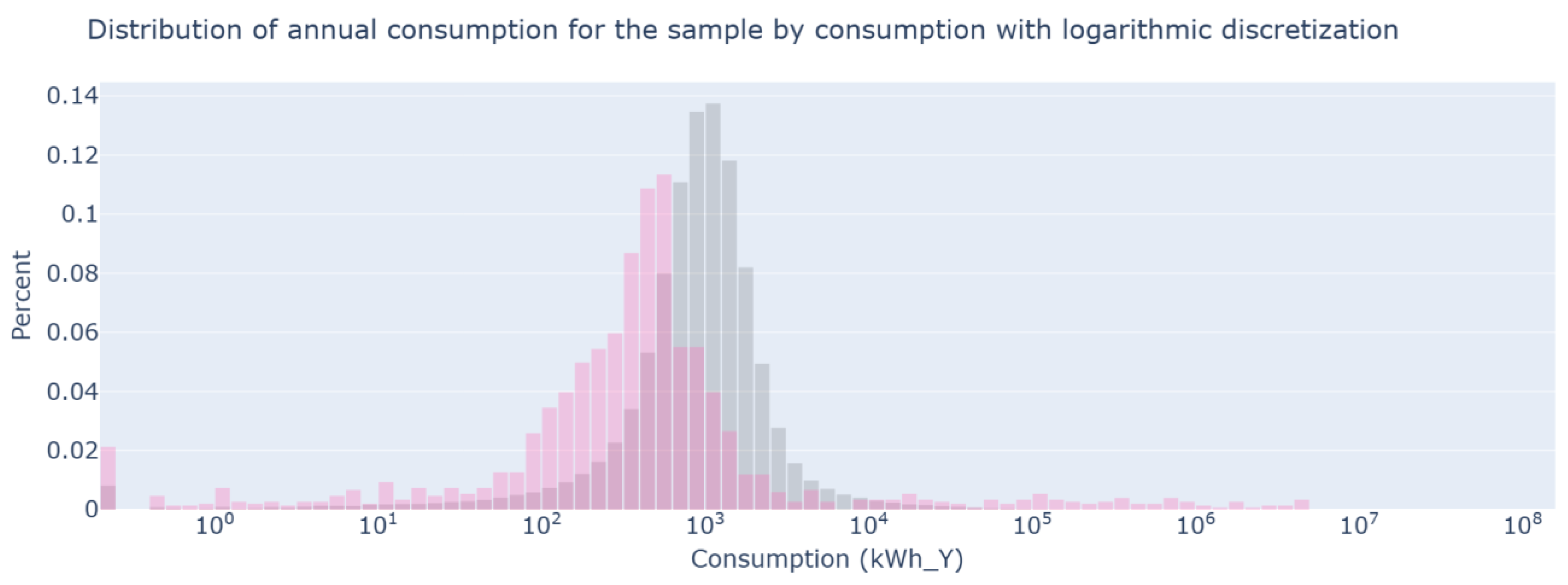
Since this strategy seeks to reconstruct the consumption curve, the analysis by subregion shows a good fit with respect to the actual consumption distribution. This is consistent with the high 95% confidence level. However, Figure 10 presents a counterintuitive result. When the four subsamples are combined to form the overall sample, the fit with respect to the consumption distribution of the entire population is poor. This may occur due to a randomness bias that the Monte Carlo method introduces into the sample. By defining any random seed, there is no guarantee that the selected random seed will offer the best results. It is possible for a random seed to offer better or worse results than any other seed when extracting users. This is a significant shortcoming because the sample fails to meet the primary objective of fitting the consumption curve, which represents the population’s energy demand. The strategy based on KL divergence seeks to improve the main weaknesses of the consumption-only strategy.

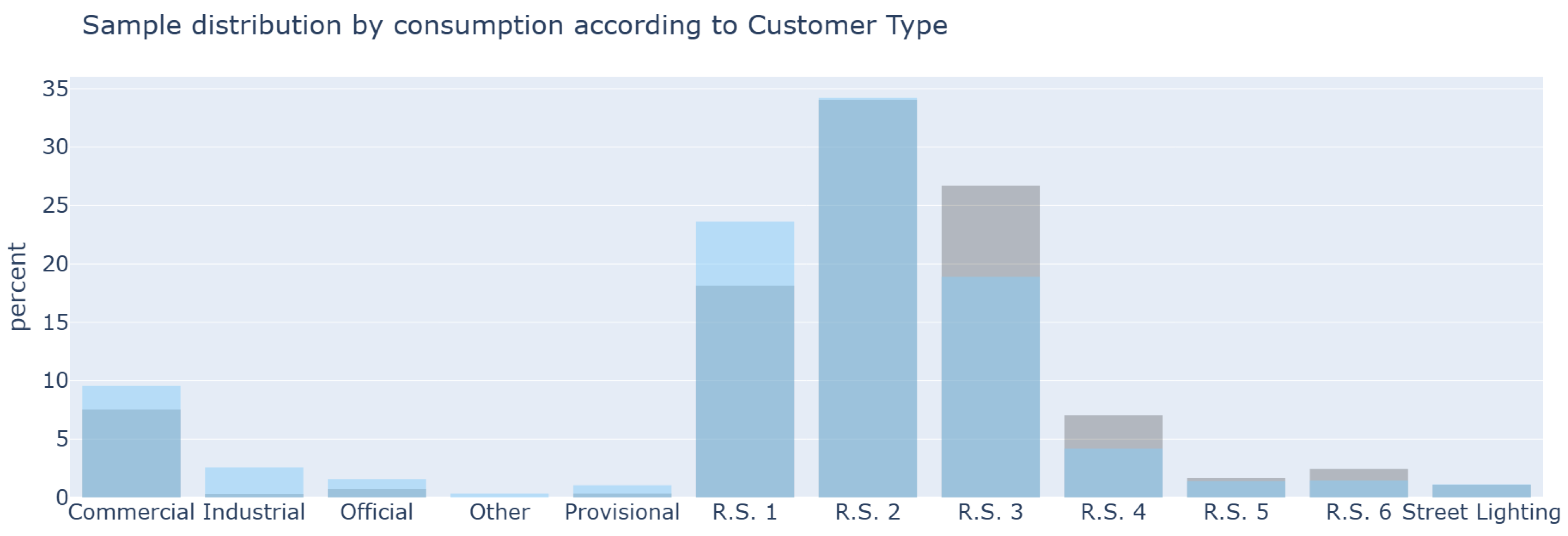
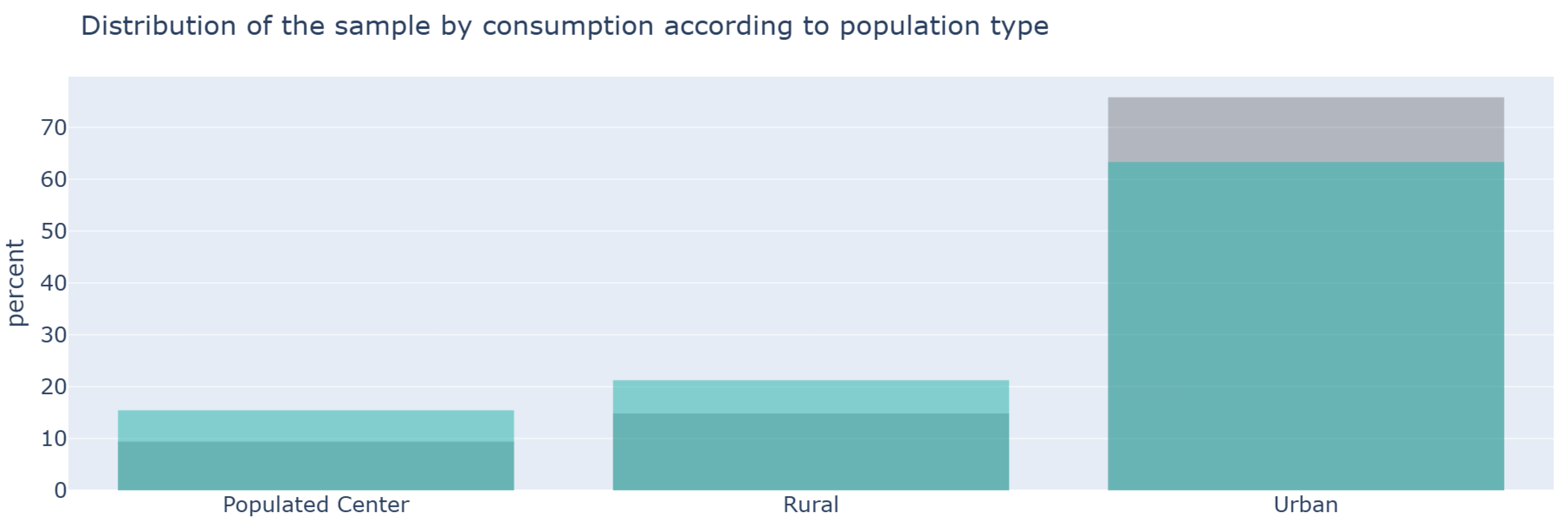
Figure 11 shows the inclusion of users from strata 4, 5, and 6, who were absent or under-represented in the entropy sample. It is also observed that users in stratum 1 are no longer as overrepresented. There is a moderate increase in commercial and industrial users thanks to the use of smoothing, which favors less frequent groups. Figure 12 shows a slight overrepresentation of users from urban and populated centers and a moderate under-representation of urban users. The fit is good for all three population types.

Table 8. Pearson correlation coefficients and p-value for the consumption sample distributions with respect to the original population.

Distribution	Correlation	p-Value
Consumption	−0.1587	0
Customer Type	0.9619	0
Population Type	0.9993	0.0234

shows the correlation coefficient values of the sample compared with those of the original population. The coefficients for the distribution of customer type and population are high, above 0.95, which reinforces what was previously described in Figure 11 and Figure 12. Likewise, the correlation coefficient confirms the poor fit of this sample with the consumption distribution, obtaining a negative coefficient of −0.1587. All the p values indicate significant relationships.

5.5. Evaluation and Results of the Sample by KL Divergence

This section presents the results of the selection strategy based on minimizing the KL divergence. Starting from an initial random sample, an iterative optimization is applied. The configuration with the lowest divergence from the original distribution is selected. This results in a representative sample in terms of energy consumption, customer type, population type, and geographic location.

A 95% confidence level was used. This level offers a good balance between sample size and representativeness. The final sample includes 1534 users. Each subregion was optimized independently. For each, multiple samples with different random seeds were generated, and their KL divergence was calculated. The sample with the lowest divergence was chosen. This process reduces the bias that random seeds can introduce. Ten thousand different samples were generated. This high number increases the probability of finding a configuration that reduces bias and improves representativeness. The optimized sample achieved a KL divergence of 0.045. This value is 40.76 times smaller than the worst case, which was 1.834.

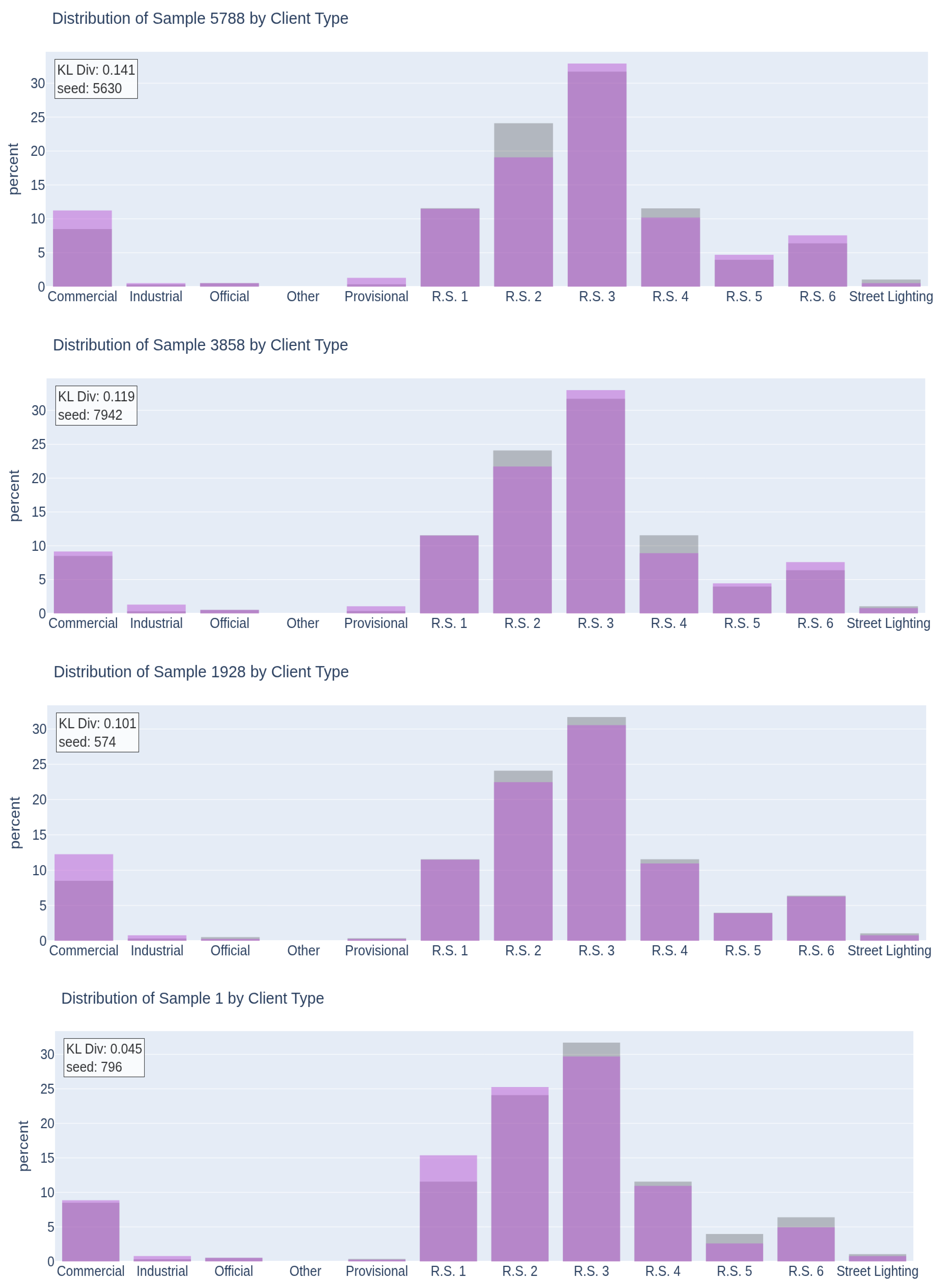
Figure 13 shows several sampling distributions (in purple) compared to the population (in gray). The 10,000 generated samples were ordered by their KL divergence. Five equidistant samples were selected, from worst to best. The last corresponds to the optimal sample. The top-down iterations show how the fit improves by customer type. The first two iterations achieve a notable improvement. From the third iteration onwards, the improvement is significantly smaller. This indicates rapid convergence toward stable configurations with similar results. The example is presented for the Center subregion. The final optimized sample has a fit very close to that of the population in this subregion. This behavior was also observed in the other subregions during the optimization process.

Table 9. Difference in proportions between population and sample based on divergence by customer type and region.

Region	S.L.	Com.	Ind.	Off.	Oth.	Prov.	R.S.1	R.S.2	R.S.3	R.S.4	R.S.5	R.S.6
North	0.02	0.02	0.21	0.13	0.00	0.06	2.77	3.69	1.08	0.20	0.13	0.19
South	0.16	0.31	0.01	0.00	0.00	0.15	1.00	1.26	0.44	0.25	0.17	0.19
Center	0.01	0.40	0.06	0.00	0.01	0.15	1.61	0.01	1.57	0.23	0.30	0.36
East	0.02	0.75	0.12	0.01	0.01	0.01	0.01	0.85	0.76	0.53	0.03	0.13
General	0.03	0.27	0.04	0.07	0.00	0.04	1.54	4.38	2.94	1.60	0.56	0.74

S.L.: Street Lighting, Com.: Commercial, Ind.: Industrial, Off.: Official, Oth.: Other, Prov.: Provisional, R.S.: Residential Strata.

and

Table 10. Difference in average distances between users and population–sample ratios by population type and region for the divergence-based sample.

Region	P. Center	Rural	Urban	Avg. Distance [km]
North	1.45	1.62	3.07	0.23
South	2.43	0.47	1.96	0.35
Center	0.55	1.28	1.83	0.02
East	2.76	0.49	3.25	2.24
General	3.89	3.63	7.52	14.31

show similar behavior to that observed in the consumption strategy. Proportions by category are presented, segmented by subregion. The fits are very good, and better representativeness of stratum 3 users is achieved. The entropy and consumption samples had limitations in achieving this level of representativeness. Table 10 reports the average distance between users. This distance increases by 14.31 km compared to the average distance for the general population. This increase is explained by the geographic conditions of the region, which create separation between the four subsamples, and by the small number of users in the sample. The differences are small when analyzing each subregion separately. The Central subregion shows only a 20-m difference. Even with this metric, the divergence sample maintains a good fit.

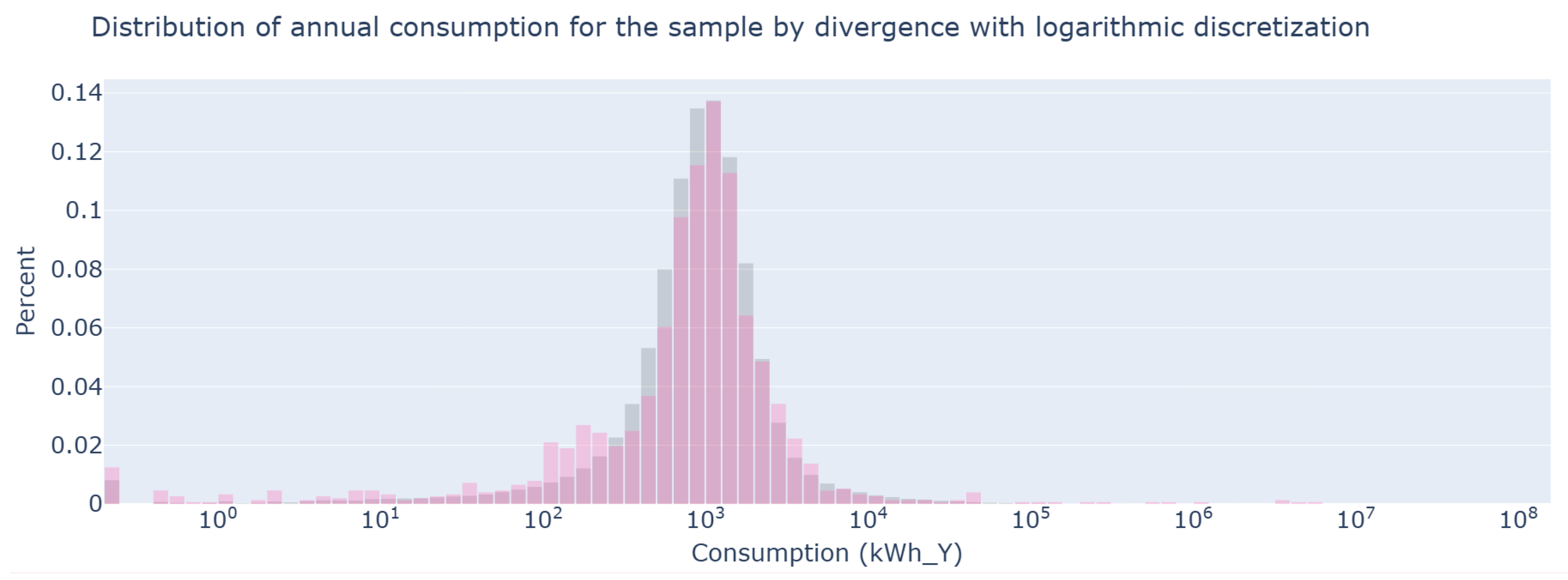
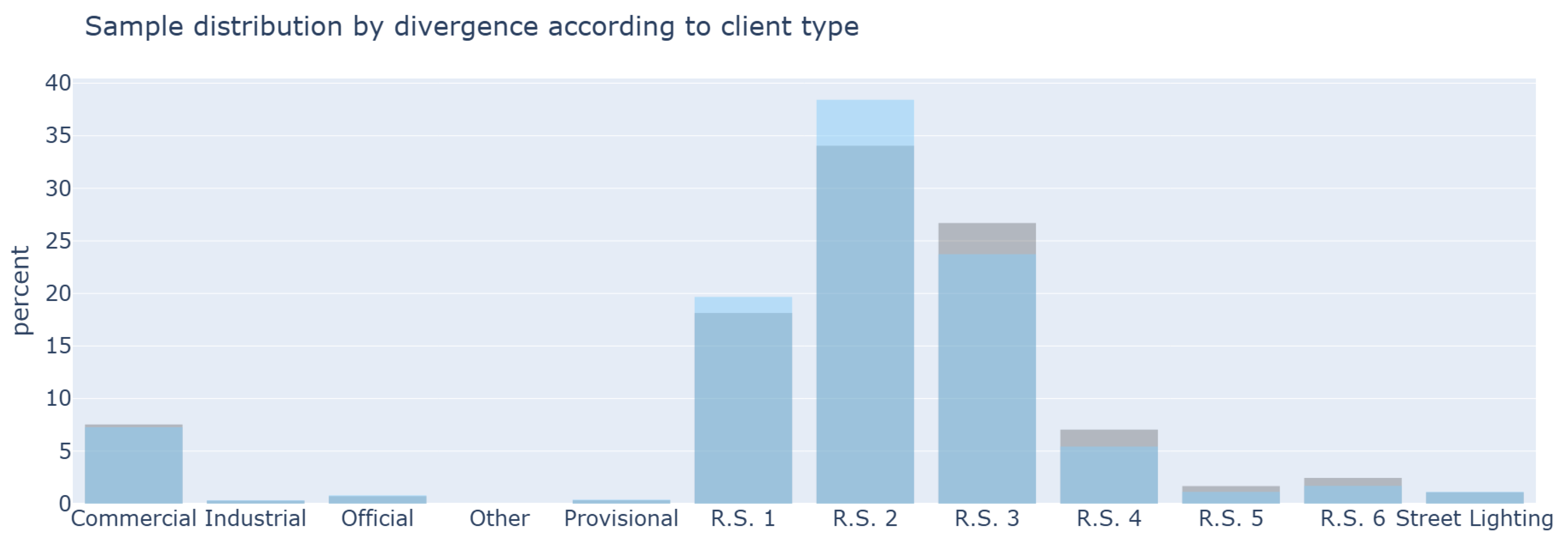
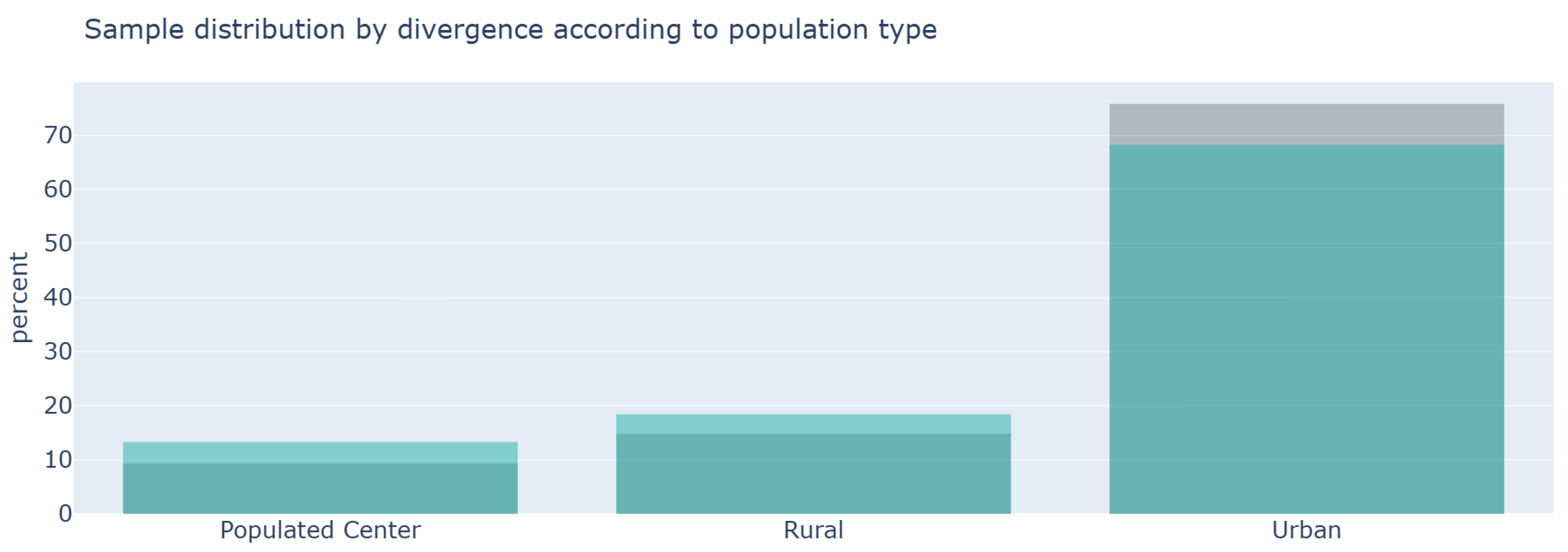
Figure 14 shows a significant improvement in the consumption distribution compared to the consumption sample presented in Figure 10. This strategy overcomes the main weakness of the previous approach. The integration of the divergence criterion evaluated by customer type also improves the sample’s representativeness of actual consumption patterns. The consumption distribution in Figure 14 presents a less pronounced peak and longer tails than the original distribution. This is due to the smoothing applied (4). Despite these effects, the sample curves retain a high similarity to the original curves. This allows the sample to adequately represent demand. Figure 15 and Figure 16 show a robust fit to the distributions by customer type and population type. These figures confirm that the sample includes both common and atypical categories. The strategy achieves a highly representative sample by including consumption and characterization categories within the selection criterion.

Table 11. Pearson correlation coefficients and p-value for the KL divergence sample distributions with respect to the original population.

Distribution	Correlation	p-Value
Consumption	0.8954	0
Customer Type	0.9913	0
Population Type	0.9999	0.0067

shows excellent values for the distributions by customer type and population, both exceeding 0.99. Furthermore, a considerable improvement in the correlation coefficient for the consumption distribution is observed in the KL sample, in contrast to the consumption-only sample. A value of 0.8954 is high and reflects a good fit with respect to the consumption curve.

In summary, the results of the KL divergence-optimized strategy show a substantial improvement in representativeness compared to the original population. This is evident in the fit of the consumption curve and the distributions by user type. The integration of multiple criteria allows for the construction of a balanced and diverse sample that clearly reflects the population structure. Although geographic dispersion increases when subsamples are consolidated, within each subregion, the average distances remain close to those of the population. This strategy represents a robust and accurate alternative for studies that require high fidelity to real distributions.

6. Discussion

This section analyzes the advantages, limitations, and recommended applications of each of the proposed sampling strategies. The flexibility, statistical quality, and geographic behavior of the samples are compared. This analysis allows for identifying which methodology best suits different operational, budgetary, and planning objectives. This is especially relevant in developing regions where a balance between representativeness and logistical efficiency is required.

The strategy based on KL divergence retains the main characteristics of consumption sampling, particularly its geographic dispersion. However, it improves the fit to the distributions by user type and consumption distribution. This is evident by comparing distribution Figure 10, Figure 11 and Figure 12 with Figure 14, Figure 15, Figure 16 and by comparing the correlation coefficients in Table 8 and Table 11. Minimizing the KL-divergence allows for greater representativeness by customer type and reduces the bias caused by suboptimal random seeds. The KL-divergence strategy maintains the advantages of the consumption-based approach and improves its results. Its only disadvantage is the greater computational burden of the iterative process that searches for the optimal sample. This increases the time required to obtain the results. Although the consumption-based strategy can be useful in rapid exploratory analyses, the KL-divergence strategy is more advisable for studies requiring high precision. For these reasons, the analysis of results will focus on comparing the Shannon entropy and KL-divergence approaches.

Firstly,

Table 12. Summary table for the comparative evaluation of Shannon entropy-based and KL divergence-based sampling strategies.

Criterion	Shannon Entropy-Based Sampling	KL Divergence-Based Sampling
Methods and Approaches	Ranks distribution transformers by Shannon entropy of categorical variables (customer type, population type), normalized by number of users to balance diversity and scale. Selection guided by adjustable weighting (e.g., 90/10) to ensure rural inclusion while prioritizing customer diversity. Deterministic selection without reliance on random seeds.	Starts with consumption-based sampling using logarithmic discretization and smoothing (β = 0.05), then generates multiple samples (0–10,000 seeds). Chooses sample minimizing KL divergence between customer type distribution of sample and population. Optimizes both categorical representativeness and consumption diversity.
Logistical Ease and Representativeness	Produces geographically clustered samples, which minimize travel distances and operational costs—ideal in regions with poor connectivity or difficult terrain. Even without using consumption directly, it achieves a strong fit to consumption distribution because categorical variables capture latent demand patterns. Allows smaller samples without losing diversity. However, tends to under-represent atypical or high-consumption users.	Generates geographically dispersed samples, increasing logistical complexity and cost, especially in low-infrastructure regions. Maintains proportional representation within each subregion and ensures inclusion of rare consumption types. Superior representativeness across both categorical and consumption variables, reducing bias toward majority groups.
Methodological Robustness	Highly robust in data-scarce contexts. Works well with incomplete or low-quality quantitative data, as it only needs categorical attributes. Less sensitive to seasonal variation or missing records. Deterministic process avoids random variability, ensuring reproducibility across runs.	Robust due to optimization step over multiple seeds, which mitigates randomness in Monte Carlo selection. Balanced treatment of common and rare consumption patterns via smoothing. However, more sensitive to parameter tuning (β, discretization) than entropy method; improper settings can skew results.
Interpretability of Results	High—relies on a familiar, transparent metric (Shannon entropy) based on understandable categories like customer type and population type. Easy to communicate to non-technical stakeholders; decision-makers can see clear logic behind transformer ranking and sample composition.	High—KL divergence provides a single, interpretable metric of sample quality relative to population. Flexible in choice of reference distribution (e.g., could target other operational variables). Slightly more technical to explain than entropy but still transparent in justifying sample selection.
Flexibility & Adaptability	Adjustable weighting between variables (e.g., 90/10, 50/50) enables tuning for different policy or operational priorities, such as increasing rural coverage or targeting specific user segments. Can incorporate new categorical dimensions without losing efficiency. On the other hand, the computational requirements of this strategy are negligible. Implementing this strategy on a consumer-grade computer took about 10 s processing a volume of 500,000 data points. The memory and time complexity is linear O(n). Computing capabilities are not an impediment.	Highly adaptable—objective function in KL divergence can be modified to target any combination of categorical or continuous variables, allowing application to tariff studies, technical interventions, or behavioral research. Subregional application facilitates integration into decentralized operational plans. Although this strategy is computationally more demanding than the others, on average each iteration of the process took about 20 s on a consumer-grade computer. The memory complexity is linear O($n$). The time complexity is linear as well O($i$⋅$n$), having $i$ iterations. Therefore, its flexibility and applicability are not greatly affected by its computing requirements.
Best Application Scenarios	When logistical simplicity and operational cost minimization are top priorities, especially in rugged or low-access regions. Suitable for quick deployment and monitoring in budget-constrained projects while maintaining acceptable representativeness.	When maximum fidelity to population structure is essential for planning, behavior analysis, or policy targeting, even at higher operational cost. Recommended for large-scale, high-accuracy studies where representativeness outweighs logistical constraints.

is presented to summarize the advantages and disadvantages of the methods and their specific applications. For this summary, four main evaluation criteria were used. The selection of the criteria—logistical ease and representativeness, methodological robustness, interpretability of results, and flexibility and adaptability—responds to both the operational realities of low-infrastructure regions and the rigor required for demand characterization. Logistical ease and representativeness are essential to ensure that samples not only reflect the true structure of the population but can also be implemented efficiently in areas with limited connectivity, difficult terrain, or budget constraints. Methodological robustness ensures that the results are consistent, reliable, and reproducible, even when faced with variations in data quality, parameter settings, or initial conditions, thereby reinforcing the validity and applicability of the study in real-world scenarios. Interpretability of results is critical for transparent communication and justification of sampling decisions, enabling stakeholders and decision-makers—often without technical backgrounds—to understand, trust, and adopt the findings. Finally, flexibility and adaptability determine the capacity of a methodology to adjust to changing objectives, constraints, or operational environments without losing effectiveness, enhancing its practical value and scalability for different contexts, objectives, and territorial scales.

After this, the obtained results will be compared and discussed with the findings and research results obtained by other authors.

At a general level, both strategies—the strategies based in entropy and KL divergence—generate samples that fit well with the general population distribution. The strategy based on divergence offers a better fit to user type distributions and greater inclusion of outliers. The entropy-based strategy provides a better fit to the consumption distribution. The main difference between them lies in the way the samples are geographically distributed within the region.

The entropy-based sampling strategy tends to form clusters of users in specific areas, especially in urban areas. Instead of covering the entire city homogeneously, the sample is concentrated in sectors such as entire neighborhoods. This pattern has been observed in recent studies using entropy analysis to identify consumption patterns in urban environments. For example, a study on water demand applied entropy and time series clustering to identify distinct residential patterns. This work showed how some areas exhibit more homogeneous consumption behaviors than others [44]. In another study on electricity demand, entropy-based metrics were used to maximize information diversity with small samples. This allowed for optimized characterization and management of residential consumption [45].

The ability of this approach to generate clusters is useful beyond the electricity sector. In contexts with logistical or budgetary constraints, it allows for the selection of a few clustered users that closely represent the population. This optimizes resource use. In environmental studies, entropy-based methods have been effective in selecting observation points that maximize the collected information, even in complex urban settings. Maximum entropy modeling has been used to select sampling sites in environmental networks. This allowed for capturing heterogeneity with few observation points [46]. Entropy criteria have also been used to optimize sensor networks in cities. These criteria allowed for the detection of hazardous emission sources with few sensors [47]. In water networks, entropy metrics helped locate a limited number of sensors that detect leaks with high efficiency [48]. In industrial contexts, an entropy-based strategy was used to estimate emission sources in chemical plants and optimize sensor placement to capture variability in operating conditions [49]. These approaches demonstrate the usefulness of entropy as a tool for designing efficient and representative monitoring networks in contexts with operational constraints.

The ability of the entropy-based strategy to form clusters that represent complex patterns makes it an effective tool for decision support in heterogeneous environments. The KL-divergence-based sampling strategy is based on capturing consumption information and offers advantages in contexts where diversity in energy behavior is a priority. This strategy allows for the identification of geographic variability and atypical profiles. It is especially useful in tariff studies where understanding how different consumption levels affect costs and subsidies is key. Research has shown that tariff designs impact socioeconomic groups differently. These studies highlight the need to adjust tariffs based on variations in consumption to distribute costs more fairly [50]. The effects of time-of-use tariffs on commercial and industrial users have also been analyzed. This research shows how these structures significantly modify costs for these sectors [51]. These findings support the use of the sampling strategy to capture consumption diversity and support the formulation of more inclusive tariff policies. It allows for the inclusion of users who are often under-represented, such as users in small towns, neighborhoods with extreme social strata, and rural areas. Recent studies highlight the importance of considering spatial variability in sampling processes. This consideration improves representativeness and reduces bias in distribution models [52]. The KL-divergence-based strategy generates samples with broad territorial coverage. This allows characterizing regions with high socioeconomic disparity and a great diversity of consumption profiles. However, this broad coverage entails greater logistical challenges and higher operating costs, especially if the implementation of sophisticated infrastructures such as AMI is sought. Although representativeness improves, the costs and complexity of collection can limit its use in projects with budgetary or logistical constraints [53]. The strategy based on divergence is adequate for studies of moderate territorial scope where statistical representativeness is a priority.

The KL-divergence-based approach also applies to sectors such as drinking water and basic sanitation. In these contexts, consumption patterns vary by urban and rural areas and by user type. Sampling that prioritizes diversity allows for more precise identification of the behavior of minority groups. This facilitates the design of more targeted and equitable cross-subsidies or conservation strategies. Studies in Brazil show that increasing block tariffs (IBT) can generate regressive subsidies if not adjusted to local socioeconomic conditions. These studies highlight the importance of tariffs that reflect consumption diversity to improve equity in water access [54,55]. In Chile, a water distribution scheme complemented by subsidies was implemented in underdeveloped regions. This policy supported customers living in poverty and demonstrated the need for tariff structures that recognize differences between residential and non-residential users [56]. In the manufacturing industry, geographic diversification of the customer base has been useful for improving inventory allocation efficiency, especially during periods of economic downturn. A study of manufacturing companies in the United States found that having a geographically diverse customer base allows for more efficient inventory sales and allocation in times of economic crisis [57]. This result demonstrates that it is possible to draw diverse samples from a population and use them as market targets. KL divergence has also been useful in artificial intelligence applications, such as in sampling schemes for non-autoregressive language models. In a study of natural language models, KL divergence was used to improve the quality and consistency of text generation by balancing diversity and fidelity [58]. These applications across different sectors highlight the versatility of the KL-divergence-based and consumption-based sampling strategy to improve representativeness, efficiency, and sustainability in diverse contexts.

The overall analysis concludes that no single strategy is superior in all respects. Each approach offers distinct advantages depending on the required balance between accuracy, diversity, coverage, and practical feasibility. The entropy-based strategy offers the best fit to the consumption curve. It is the most appropriate option when there are logistical constraints, as it concentrates information users in specific areas. The KL-divergence-based strategy excels at capturing the diversity of profiles across the region and is the most robust in terms of representativeness. The latter is the most comprehensive option when statistical accuracy and territorial coverage are the priority, provided the necessary operational resources are available.

7. Conclusions

This study addressed the hypothesis that it is possible to construct representative and operationally viable energy demand samples in regions without AMI, through the integration of entropy-based, consumption-based, or divergence-minimizing sampling strategies. The results obtained confirm this and provide guidance for low-infrastructure contexts in Colombia.

• Considering the objective of offering flexible tools for demand characterization in contexts with limited infrastructure, the KL-divergence strategy is the best option for the grid operator. This strategy yields near-perfect correlation with customer (r = 0.9913, p = 0) and population type distributions (r = 0.9999, p = 0.0067), while maintaining good correlation with consumption distribution (r = 0.8954, p = 0). By optimizing across multiple seeds, it minimizes sampling bias and ensures representativeness in both consumption and user categories. Despite higher logistical costs from spatial dispersion, it balances statistical accuracy and territorial coverage, with a KL divergence of 0.045 and an average user distance difference of 14.31 km. For these reasons, it is recommended when characterization quality is a priority.
• The entropy strategy achieved perfect correlation between entropy and consumption distribution (r = 1.0000, p < 0.001) without using consumption as a criterion. It is highly efficient logistically, thanks to geographic clustering. This lowers costs in remote areas, with an average distance difference of 11.48 km. Its limitation is poor representativeness of atypical profiles, reducing its value for comprehensive studies. It is best suited when logistical efficiency is prioritized, especially if complemented by including categories with greater informational diversity.
• In terms of robustness and adaptability, entropy and KL-divergence strategies provide reliable but distinct approaches. Entropy sampling, based on categorical variables, is less affected by measurement errors or missing data, fitting limited-infrastructure contexts. KL divergence is more versatile, handling continuous and categorical variables while preserving multiple population dimensions. It quickly converges to similar solutions across random seeds. This ensures consistency in the strategy results. Both are highly interpretable, using familiar variables and clear metrics that aid communication and support institutional adoption, particularly in public-sector planning requiring technical justification for territorial targeting.
• The consumption-based method includes atypical profiles and broad geographic coverage but is more sensitive to random seed bias and shows weaker correlation with consumption than other methods. It is better for quick exploratory analyses, while the KL-divergence approach is preferable for more rigorous studies.

There is no universally optimal strategy; each balances logistical constraints, representativeness, and analytical capacity differently. This work provides a comparative framework to help grid operators select and adapt sampling methods to their conditions and objectives.

7.1. Recommendations for Decision-Makers

For grid operators and policy-makers without AMI, the KL-divergence strategy is most suitable when precision and broad representation are priorities. Its ability to capture consumption patterns and its multiple qualitative categories of the population make it valuable for planning, tariff design, and policy evaluation, although it could risk inefficiency. In contrast, the entropy-based strategy fits contexts prioritizing cost-efficiency and logistics, such as remote areas, by clustering users to reduce travel, installation, and maintenance costs.

7.2. Limitations

While the study confirms the feasibility of building representative samples from conventional metering data, several limitations must be noted. The analysis uses only monthly consumption records, missing finer temporal variability such as daily profiles or short-term peaks that affect grid operations. Without AMI-based validation, the strategies cannot yet be benchmarked against real-time behavior, limiting forecast precision. Results also reflect the Colombian case study’s socio-economic mix, grid topology, and rural–urban structure, which may not generalize elsewhere without adaptation. Moreover, the models exclude seasonal effects, demand shifts, or behavioral changes from policy measures. These factors underscore the need for context-specific calibration before broader application.

7.3. Future Research Directions

Future research should integrate geospatial optimization to minimize travel and logistics while preserving representativeness. Testing the strategies in other developing regions will clarify transferability and scalability. Synthetic high-frequency data or partial AMI could enable validation under more detailed consumption dynamics. Future work could examine hybrid optimization methods that merge entropy metrics and divergence, adjusting the categories weighting and evaluating which of these categories optimizes the divergence of the resulting sample. A multi-objective framework may yield adaptable, resource-efficient sampling solutions aligned with both budgetary and analytical needs.

References

1. Inter-American Development Bank. Medición Inteligente en América Latina y el Caribe: Recomendaciones Regulatorias para Avanzar su Implementación; Technical Report; IDB: Washington, DC, USA, 2022. [Google Scholar]
2. Khan, I.; Tareen, M.; Sial, M.N. A survey-based electricity demand profiling method for developing countries: The case of urban households in Bangladesh. J. Build. Eng. 2021, 42, 102507. [Google Scholar] [CrossRef]
3. World Bank. Smartening the Grid in Developing Countries: Emerging Lessons from World Bank Lending; Live Wire 2016/67; World Bank: Washington, DC, USA, 2016. [Google Scholar]
4. Garcés, E.; Rivera, J.; Henao, A.; Pachón, J. Lessons from last mile electrification in Colombia: Examining the policy framework and outcomes for sustainability. Energy Res. Soc. Sci. 2021, 80, 102232. [Google Scholar]
5. Gutiérrez, S.M.T.; García, J.R.; Gandarillas, R.C. Sistemas de medición avanzada en Colombia: Beneficios, retos y oportunidades. Ing. Desarro. 2018, 36, 469–488. [Google Scholar] [CrossRef]
6. Viscidi, L. Peace in Colombia’s Countryside? First, Turn on the Lights. Americas Quarterly. November 2017. Available online: https://www.americasquarterly.org/fulltextarticle/peace-in-colombias-countryside-first-turn-on-the-lights (accessed on 7 July 2025).
7. Carrillo Romero, J.L.; Perdomo Arias, A.F. Caracterización y Análisis del Consumo Energético en Zonas Rurales Para Los Municipios de Arauca; Universidad de los Llanos: Villavicencio, Colombia, 2017. [Google Scholar]
8. Swan, L.G.; Ugursal, V.I. Modeling of end-use energy consumption in the residential sector: A review of modeling techniques. Renew. Sustain. Energy Rev. 2009, 13, 1819–1835. [Google Scholar] [CrossRef]
9. Auder, B.; Cugliari, J.; Goude, Y.; Poggi, J.M. Scalable Clustering of Individual Electrical Curves for Profiling and Bottom-Up Forecasting. Energies 2018, 11, 1893. [Google Scholar] [CrossRef]
10. Huang, Y.; Zhan, J.; Wang, N.; Luo, C.; Wang, L.; Ren, R. Clustering Residential Electricity Load Curves via Community Detection in Network. arXiv 2018, arXiv:1811.10356. [Google Scholar] [CrossRef]
11. Alonso, A.M.; Nogales, F.J.; Ruiz, C. Hierarchical Clustering for Smart Meter Electricity Loads Based on Quantile Autocovariances. arXiv 2019, arXiv:1911.03336. [Google Scholar] [CrossRef]
12. Cordeiro-Costas, M.; Villanueva, D.; Eguía-Oller; Martínez-Comesaña, M.; Ramos, S. Load Forecasting with Machine Learning and Deep Learning Methods. Appl. Sci. 2023, 13, 7933. [Google Scholar] [CrossRef]
13. Douaidi, L.; Senouci, S.M.; El Korbi, I.; Harrou, F. Predicting Electric Vehicle Charging Stations Occupancy: A Federated Deep Learning Framework. In Proceedings of the 2023 IEEE 97th Vehicular Technology Conference (VTC2023-Spring), Florence, Italy, 20–23 June 2023; pp. 1–5. [Google Scholar] [CrossRef]
14. Genes, C.; Esnaola, I.; Perlaza, S.M.; Ochoa, L.F.; Coca, D. Robust Recovery of Missing Data in Electricity Distribution Systems. arXiv 2017, arXiv:1708.01583. [Google Scholar] [CrossRef]
15. Huang, Y.; Hasan, N.; Deng, C.; Bao, Y. Multivariate empirical mode decomposition based hybrid model for day-ahead peak load forecasting. Energy 2022, 239, 122245. [Google Scholar] [CrossRef]
16. Zhang, J.; Wei, Y.M.; Li, D.; Tan, Z.; Zhou, J. Short term electricity load forecasting using a hybrid model. Energy 2018, 158, 774–781. [Google Scholar] [CrossRef]
17. Sina, A.; Kaur, D. An Accurate Hybrid Approach for Electric Short-Term Load Forecasting. IETE J. Res. 2021, 69, 2727–2742. [Google Scholar] [CrossRef]
18. Saxena, H.; Aponte, O.; McConky, K.T. A hybrid machine learning model for forecasting a billing period’s peak electric load days. Int. J. Forecast. 2019, 35, 1288–1303. [Google Scholar] [CrossRef]
19. Uparela, M.A.; Gonzalez, R.D.; Jimenez, J.R.; Quintero, C.G. Intelligent system for non-technical losses management in residential users of the electricity sector. Ing. Investig. 2018, 38, 52–60. [Google Scholar] [CrossRef]
20. Rahimpour, A.; Qi, H.; Fugate, D.; Kuruganti, T. Non-Intrusive Energy Disaggregation Using Non-Negative Matrix Factorization With Sum-to-k Constraint. IEEE Trans. Power Syst. 2017, 32, 4430–4441. [Google Scholar] [CrossRef]
21. Norte, S.; José, S.; Tortós, J.Q. Metodología para la Determinación de Curvas de Carga y Consumo Eléctrico Residencial por Uso—Informe Final; Escuela de Ingeniería Eléctrica, Universidad de Costa Rica, Informe Final para el Instituto Costarricense de Electricidad: San José, CR, USA, 2019. [Google Scholar]
22. Yarba, I.Y.; Çelik, A.K. The determinants of household electricity demand in Turkey: An implementation of the Heckman Sample Selection model. Energy 2023, 283, 128431. [Google Scholar] [CrossRef]
23. Pavón, C.; Barzola-Monteses, J. Estimación de la Demanda Energética Mensual Mediante Encuesta Aplicada en la Provincia de Santa Elena. Available online: https://www.researchgate.net/publication/309286132 (accessed on 7 July 2025).
24. Imberg, H.; Yang, X.; Flannagan, C.; Bärgman, J. Active Sampling: A Machine-Learning-Assisted Framework for Finite Population Inference with Optimal Subsamples. Technometrics 2024, 67, 46–57. [Google Scholar] [CrossRef]
25. Reina García, J.; Peña Varón, M.R. Diseño Metodológico Para la Selección de Sitios de Muestreo en Una Red de Monitoreo de Micro–Contaminantes en Ríos de Valle: Caso de Estudio río Cauca; Food and Agriculture Organization of the United Nations: Rome, Italy, 2019. [Google Scholar]
26. Rafiee, H.; Abin, A.A.; Majd, S.S. Cluster Sampling: A Cluster-Driven Sampling Strategy for Deep Metric Learning. In Proceedings of the 2024 14th International Conference on Computer and Knowledge Engineering (ICCKE), Mashhad, Iran, 19 November 2024; pp. 460–465. [Google Scholar] [CrossRef]
27. Chen, S.; Zheng, J.; Li, J. The Impact of Sample Size after Sampling on the Accuracy of Machine Learning Models. In Proceedings of the 2024 International Conference on Computers, Information Processing and Advanced Education (CIPAE), Ottawa, ON, Canada, 26–28 August 2024; pp. 61–66. [Google Scholar] [CrossRef]
28. Zhu, Q.-X.; Zhao, Q.-Q.; Xu, Y.; He, Y.-L. Novel virtual sample generation using Gibbs Sampling integrated with GRNN for handling small data in soft sensing. In Proceedings of the 2023 IEEE 12th Data Driven Control and Learning Systems Conference (DDCLS), Xiangtan, China, 12–14 May 2023; pp. 89–94. [Google Scholar] [CrossRef]
29. LeCun, Y.; Bengio, Y.; Hinton, G. Deep learning. Nature 2015, 521, 436–444. [Google Scholar] [CrossRef]
30. Sun, X.; Li, X.; Datta, S.; Ke, X.; Huang, Q.; Huang, R.; Hou, Z.J. Smart Sampling for Reduced and Representative Power System Scenario Selection. IEEE Open Access J. Power Energy 2021, 8, 241–251. [Google Scholar] [CrossRef]
31. Asghari, P.; Zakariazadeh, A.; Siano, P. Selecting and prioritizing the electricity customers for participating in demand response programs. IET Gener. Transm. Distrib. 2022, 16, 2086–2096. [Google Scholar] [CrossRef]
32. Muhwezi, B.; Williams, N.J.; Taneja, J. Ingredients for growth: Examining electricity consumption and complementary infrastructure for Small and Medium Enterprises in Kenya. Dev. Eng. 2021, 6, 100072. [Google Scholar] [CrossRef]
33. Zhu, X.; Mather, B. Data-Driven Load Diversity and Variability Modeling for Quasi-Static Time-Series Simulation on Distribution Feeders. In Proceedings of the 2019 IEEE Power & Energy Society General Meeting (PESGM), Atlanta, GA, USA, 4–9 August 2019; pp. 1–5. [Google Scholar] [CrossRef]
34. Bañales, S.; Dormido, R.; Duro, N. Smart Meters Time Series Clustering for Demand Response Applications in the Context of High Penetration of Renewable Energy Resources. Energies 2021, 12, 3458. [Google Scholar] [CrossRef]
35. Narayan, N.; Qin, Z.; Popovic-Gerber, J.; Diehl, J.C.; Bauer, P.; Zeman, M. Stochastic load profile construction for the multi-tier framework for household electricity access using off-grid DC appliances. Energy Effic. 2020, 13, 197–215. [Google Scholar] [CrossRef]
36. Ye, X.; Esnaola, I.; Perlaza, S.M.; Harrison, R.F. An information theoretic metric for measurement vulnerability to data integrity attacks on smart grids. IET Smart Grid 2024, 7, 583–592. [Google Scholar] [CrossRef]
37. Shen, C.; Liu, H.; Wang, J.; Yang, Z.; Hai, C. Kullback–Leibler Divergence-Based Distributionally Robust Chance-Constrained Programming for PV Hosting Capacity Assessment in Distribution Networks. Sustainability 2025, 17, 2022. [Google Scholar] [CrossRef]
38. Shannon, C.E. A Mathematical Theory of Communication. Bell Syst. Tech. J. 1948, 27, 379–423, 623–656. [Google Scholar] [CrossRef]
39. Ahmed, S.K. How to choose a sampling technique and determine sample size for research: A simplified guide for researchers. Oral Oncol. Rep. 2024, 12, 100662. [Google Scholar] [CrossRef]
40. Liu, H.; Hussain, F.; Tan, C.L.; Dash, M. Discretization: An Enabling Technique. Data Min. Knowl. Discov. 2002, 6, 393–423. [Google Scholar] [CrossRef]
41. Manning, C.D.; Raghavan; Schütze, H. Introduction to Information Retrieval; Cambridge University Press: Cambridge, UK, 2008; p. 260. [Google Scholar]
42. Cover, T.M. Elements of Information Theory, 2nd ed.; Wiley: Hoboken, NJ, USA, 2006; p. 80. [Google Scholar]
43. Kullback, S.; Leibler, R. On Information and Sufficiency. Ann. Math. Stat. 1951, 22, 79–86. [Google Scholar] [CrossRef]
44. Wang, R.; Zhao, X.; Qiu, H.; Cheng, X.; Liu, X. Uncovering urban water consumption patterns through time series clustering and entropy analysis. Water Res. 2024, 262, 122085. [Google Scholar] [CrossRef] [PubMed]
45. Stohlgren, T.J.; Kumar, S.; Barnett, D.T.; Evangelista, P.H. Using Maximum Entropy Modeling for Optimal Selection of Sampling Sites for Monitoring Networks. Diversity 2011, 3, 252–261. [Google Scholar] [CrossRef]
46. Ngae, P.; Kouichi, H.; Kumar, P.; Feiz, A.A.; Chpoun, A. Optimization of an urban monitoring network for emergency response applications: An approach for characterizing the source of hazardous releases. Q. J. R. Meteorol. Soc. 2019, 145, 967–981. [Google Scholar] [CrossRef]
47. Khorshidi, M.S.; Nikoo, M.R.; Sadegh, M. Optimal and objective placement of sensors in water distribution systems using information theory. Water Res. 2018, 143, 218–228. [Google Scholar] [CrossRef]
48. Tian, H.; Lang, Z.; Cao, C.; Wang, B. Optimizing Sensor Placement for Enhanced Source Term Estimation in Chemical Plants. Processes 2025, 13, 825. [Google Scholar] [CrossRef]
49. Hock, D.; Kappes, M.; Ghita, B. Entropy-Based Metrics for Occupancy Detection Using Energy Demand. Entropy 2020, 22, 731. [Google Scholar] [CrossRef]
50. Gunkel, P.A.; Bergaentzlé, C.M.; Keles, D.; Scheller, F.; Jacobsen, H.K. Grid tariff designs coping with the challenges of electrification and their socio-economic impacts. arXiv 2022, arXiv:2210.03514. [Google Scholar] [CrossRef]
51. Smith, L.D.; Kirschen, D.S. Impacts of Time-of-Use Rate Changes on the Electricity Bills of Commercial Consumers. arXiv 2021, arXiv:2105.07106. [Google Scholar] [CrossRef]
52. Ezhilarasi, P.; Ramesh, L.; Sanjeevikumar, P.; Khan, B. A cost-effective smart metering approach towards affordable deployment strategy. Sci. Rep. 2023, 13, 19452. [Google Scholar] [CrossRef]
53. Ezhilarasi, P.; Ramesh, L.; Sanjeevikumar, P.; Khan, B. Optimal water tariffs for domestic, agricultural and industrial use. Ann. Oper. Res. 2024, 337, 1135–1165. [Google Scholar] [CrossRef]
54. Narzetti, D.A.; Marques, R.C. Models of subsidies for water and sanitation services for vulnerable people in South American countries: Lessons for Brazil. Water 2020, 12, 1976. [Google Scholar] [CrossRef]
55. Fraga, C.I.; Alves, C.D. Subsidies and affordability: A social approach to water supply tariffs. J. Water Sanit. Hyg. Dev. 2025, 15, 75–83. [Google Scholar] [CrossRef]
56. Errázuriz, C.; Gómez-Lobo, A. A new look at the distributive incidence of Chile’s means-tested water subsidy scheme. J. World Water Counc. Water Policy 2024, 26, 685–706. [Google Scholar] [CrossRef]
57. Ke, J.Y.; Otto, J.; Han, C. Customer-country diversification and inventory efficiency: Comparative evidence from the manufacturing sector during the pre-pandemic and the COVID-19 pandemic periods. J. Bus. Res. 2022, 148, 292–303. [Google Scholar] [CrossRef]
58. Sevriugov, E.; Oseledets, I. KL-geodesics flow matching with a novel sampling scheme. arXiv 2024, arXiv:2411.16821. [Google Scholar] [CrossRef]
Figure 1. The methodology receives the grouped users as input and uses several variables to generate a ranking of transformers from the most informative to the least informative. A sample is generated as output from this ranking. The methodology parameters are highlighted in purple.
Applsci 15 09588 g001
Figure 2. The methodology takes user consumption data as input and uses logarithmic discretization and smoothing to generate a discrete distribution. This distribution is used to output a user-by-user random sample. Parameters are highlighted in purple.
Applsci 15 09588 g002
Figure 3. Diagram of the KL divergence sampling process. It highlights the iterative process in which a sample is generated for n different random seeds, whose KL divergence is calculated based on the customer type. The final output is the sample with the greatest divergence from the population.
Applsci 15 09588 g003
Figure 4. Anonymized maps of the sample distribution using entropy at 95% confidence intervals and customer type/population type weights of 90/10. (a) Map of the region segmented by subregion. (b) Map of a major city segmented by customer type.
Applsci 15 09588 g004
Figure 5. Anonymized maps of the sample distribution by consumption at a 95% confidence level. (a) Map of the region segmented by subregion. (b) Map of a major city segmented by customer type.
Applsci 15 09588 g005
Figure 6. Anonymized maps of the sample distribution by 95% confidence interval. (a) Map of the region segmented by subregion. (b) Map of a major city segmented by customer type.
Applsci 15 09588 g006
Figure 7. Comparison of entropy distribution based on annual consumption. Population distribution on grey, sample distribution on pink.
Applsci 15 09588 g007
Figure 8. Comparison of entropy distribution based on customer type. Population distribution on grey, sample distribution on blue.
Applsci 15 09588 g008
Figure 9. Comparison of entropy distribution based on population type. Population distribution on grey, sample distribution on green.
Applsci 15 09588 g009
Figure 10. Comparison of distribution by consumption based on annual consumption. Population distribution on grey, sample distribution on pink.
Applsci 15 09588 g010
Figure 11. Comparison of distribution by consumption based on customer type. Population distribution on grey, sample distribution on blue.
Applsci 15 09588 g011
Figure 12. Comparison of consumption distribution based on population type. Population distribution on grey, sample distribution on green.
Applsci 15 09588 g012
Figure 13. Progression of the adjustment of the distribution by client type of the ranking of samples and their associated seeds according to their KL divergence for the Central subregion. Population distribution on grey, sample distribution on purple.
Applsci 15 09588 g013aApplsci 15 09588 g013b
Figure 14. Comparison of distribution by divergence based on annual consumption. Population distribution on grey, sample distribution on pink.
Applsci 15 09588 g014
Figure 15. Distribution comparison by divergence based on customer type. Population distribution on grey, sample distribution on blue.
Applsci 15 09588 g015
Figure 16. Comparison of distribution by divergence according to population type. Population distribution on grey, sample distribution on green.
Applsci 15 09588 g016