Energy Analysis in Green Building via Machine Learning: A Case Study in a Hospital

Abstract

Electricity consumption is increasing as a result of increasing people’s needs, such as lighting, heating, and comfort. Different needs come into play day by day in the houses where people live and in places used as common areas, and this increases the need for electricity. Studies have observed that almost half of the world’s electricity consumption is made by buildings. Public buildings, shopping malls, hospitals, and hotels are typical examples of such structures. However, hospitals have an important place among all building types as they contain a wide range of devices and are of critical importance to many systems. Consumption in hospitals is a necessity rather than a desire for comfort in places such as hotels and shopping malls. Therefore, analysis of the energy consumed by hospitals is one of the important things to perform to reduce the damage caused by electricity consumption to the environment. In this study, the energy analysis of a green hospital with an installed area of 55,000 square meters in Istanbul was conducted, and machine learning techniques can be used in the analysis. Among many methods used for building energy analysis, long short-term memory (LSTM) has been chosen. The available data set was analyzed with the various LSTM methods and classification and prediction operations were carried out. Error rates for each method were compared. With the results obtained, it has been observed that the vanilla LSTM method provides acceptable results in building energy analysis.

1. Introduction

In recent years, due to the worldwide climate crisis, measures have been taken one after another in the energy sector. Events, such as changing average temperatures due to global warming, waste released during energy production, and the depletion of natural resources, have led to the formation of some standards in the energy sector. Therefore, environmentally friendly systems have come to the fore and, as a result, the green building concept has emerged. Green buildings are also referred to as sustainable buildings, ecological buildings, and energy-efficient buildings. These terms mean that buildings exhibit high performance throughout their lifetime and cause little harm to the environment. More than 40% of the energy used in the world is spent in buildings [1]. In this study, energy analysis was conducted in a hospital with a green building.

One of the most important steps to be taken to optimize energy consumption in a building is energy analysis. Data science and machine learning have come to the fore in recent years in energy analysis in buildings [2]. The number of articles using machine learning techniques has been on a steady rise in recent years [3]. Predicting building energy loads is an application of big data science. Analyzes, such as building load estimation and determination of the relationship between energy load and consumption, can be made. Depending on the type of analysis to be performed, options such as classification, regression, or clustering can be used. There are many machine learning methods that can be used for these processes. Some of these are long short-term memory (LSTM), support vector machines (SVMs), and group method of data handling (GMDH).

One of the most effective and easiest methods to increase efficiency and save energy in electrical energy systems is reactive power compensation. Another valid way to improve energy quality is to examine and eliminate the negative effects of harmonic components. With the development of semiconductor elements, the use of rectifiers has increased and as a result, harmonic distortions have begun to be seen in electrical installations today [4].

There are many factors that affect energy consumption levels in the hospital subject of the study. While the density of people generally increases on weekdays, it decreases on weekends or public holidays. On the other hand, the density of patients and visitors changes during the day. While the hospital is very full during some hours, it may be relatively empty at other times. In addition, the most important reason for the increase and decrease in energy consumption is the devices used in the hospital. Among these devices, those that draw particularly high loads and operate only at certain times are the main reasons that cause fluctuations and harmonic distortions in the system.

The hospital in our study consists of a 19-story building with an area of 55,000 square meters and contains many different outpatient clinics and health units. There is one absorption chiller and three centrifugal chillers used for energy and air conditioning purposes in the hospital. In addition, more than 40 air handling units, air conditioning systems with HEPA filters in certain areas, a fully equipped operating room consisting of 19 different units and sleep-wake-up units, fire pump systems, and jet-fans ready to be used in emergencies are some of the factors that enable the hospital to reach high consumption values. In addition, in some parts of the hospital, especially in radiology, there are devices that draw high energy when used, such as X-ray machines, MRI machines, and PET MRIs. Energy levels constantly change throughout the day as such devices and units are used and turned off as needed. This causes harmonic distortions and an increase in the total harmonic distortion (THD) value in the hospital’s main distribution panel. In order to solve the problem, there is a compensation room in the hospital.

Many studies on energy analysis have been published in recent years. Vincent J. L. Gan et al. created a collage of simulation studies on energy efficiency in green buildings [5]. M. H. Elnabawi et al. investigated the quality of data transfer in green buildings where data were obtained through energy analysis [6]. A. D. Pham et al. estimated energy consumption in various buildings using machine learning in order to improve energy efficiency and sustainability [7]. M Shao et al. studied and analyzed the energy consumption of hotel buildings by establishing an SVM energy consumption prediction model [8]. This work found that, although the SVM model shows a high prediction accuracy, in the modeling process, the energy consumption of the buildings is greatly affected by factors such as the flow of people. Y Liu et al. estimated energy consumption in public buildings in China [9]. Son H. et al. published a study to predict the cost performance of a building with SVM [10]. Paudel S. et al. conducted a study to predict energy consumption in a low-cost building [11]. Li Q et al. predicted the hourly cooling load of a building in their study [12]. Zhao H X et al. used parallel SVM to predict energy consumption [13]. Additionally, various analysis studies using SVM are also available in the literature [14].

It can be seen that the SVM method is generally used for energy analysis and estimation in buildings. We will use the LSTM method in this study. There are also studies involving the LSTM method in energy analysis in buildings. Wang et al. performed an LSTM-based long-term energy prediction in their paper [15]. T. Le et al. published a study to improve energy consumption prediction using LSTM [16]. P Jiang et al. worked on energy prediction of industrial robots on LSTM [17]. TY Kim et al. predicted residential energy consumption with LSTM in their paper [18]. A summary of studies on various predictions, comparisons, and similar works using different machine learning models is listed in

Table 1. Purpose, content, and model information of studies on machine learning.

Study	Location	Year	Model	Monitoring Period	Error Rate
[6]	United States	2020	Random Forests	12 months	0.612
[8]	Singapore	2005	Support Vector Machine	2 years	0.14
[9]	China	2020	Support Vector Machine	3 months	0.0503
[12]	China	2009	Support Vector Machine	6 months	0.02365
[13]	France	2010	Support Vector Machine	5 months	0.0023
[15]	China	2020	Long Short-term Memory	5 months	0.197
[16]	France	2019	Convolutional Neural Network Long Short-term Memory	5 years	0.065
[18]	France	2019	Convolutional Neural Network Long Short-term Memory	4 years	0.3738

.

When it comes to big data in modeling studies, classical methods may not be sufficient. For this reason, we used machine learning methods in this study. We aim to analyze the energy data in a hospital with green building status by interpreting it with one of the machine learning techniques, LSTM. There are many similar studies in the literature on related topics. However, to the authors’ knowledge and experiences during this study, research based on the LSTM method to analyze energy in green buildings was not met. There are many studies on energy analysis in green buildings [19,20,21,22,23,24,25], but these studies include analysis with methods other than artificial intelligence or machine learning techniques and address building types far from the hospital example in this study. In our study, three main subjects stand out. These are LSTM, green building, and energy analysis. Generally, studies in this field do not include all three areas. In many studies, energy analysis performed with machine learning characterizes cities, suburbs, or a specific region. Some studies focused on energy analysis in green buildings, but machine-learning techniques were not used. Additionally, articles related to green buildings generally focus on the building’s structure, insulation, and material type. The difference in our study from others is that it collects the topics of machine learning method LSTM, green building, and energy analysis in a single article and presents a suitable study.

In this study, energy data taken from a hospital in Istanbul was analyzed with some LSTM machine-learning methods. The time period used in the study is 14 March–11 June 2023. The reason for choosing this interval is that it is one of the most intensive periods of the year when the hospital and its devices operate. After debugging and simplifying the data, a data set consisting of 779,280 rows and 102 columns remained. With the analysis studies carried out on this data set, the change in the harmonic values of the hospital was observed. Total power factor (TPF) values were estimated with these methods.

2. Materials and Methods

In this study, the energy data in a hospital with green building status will be analyzed by interpreting it with machine learning techniques. The data received with the Siemens PAC 4200 energy analyzer located on the main distribution panel of the hospital will be interpreted. The data set consists of 103 different parameters, including voltage, current, power, energy, THD, TPF, harmonic voltage (1st, 3rd, 5th, 7th, 9th, 11th), and harmonic current (1st, 3rd, 5th, 7th, 9th, 11th). The relevant values were taken every 10 s for approximately 2 months. The time range of the data used in the study is between 14 March 2023 00.00.00 and 11 June 2023 23.59.50. After debugging and simplifying the data, a data set consisting of 779,280 rows and 102 columns remained. The matrix dimensions of the data set are 102 × 779,280, which means we have a data set consisting of 79,486,560 pieces of data.

Nowadays, large data sets are used in many fields for different purposes. Manual processing of this data leads to great waste of time and perhaps errors. For this reason, machine learning has gained an important place in our lives in order to interpret large data sets quickly and accurately. There are different categories for machine learning, like supervised, unsupervised, etc. Classification and regression tasks can be applied with machine learning methods. Although these two tasks seem to be the same, they have a fundamental difference. The prediction task, in which the data set is discrete, is called classification. If the data are continuous, it is called regression. In this study, the classification process, which is a supervised learning prediction task, will be applied to the data set we have.

Classification is a supervised machine learning method, in which an attempt is made to predict the correct label of a given input data. A model is created in classification. The created model is fully trained using the training data. The model is then evaluated on test data and used for prediction. Models, such as SVM, nearest neighbor, and neural networks, can be used in classification. There are different types of artificial neural networks. Recurrent neural network (RNN) is one of the frequently used types of artificial neural networks. LSTM network is the name of a method of this type. In this study, the data set will be trained with the LSTM model.

2.1. Long Short-Term Memory for Time Series Forecasting

The LSTM network is a type of RNN. It acts as a short-term memory consisting of many time steps combined. In data analysis operations, it is processed for classification and prediction purposes. LSTM is a method used in applications where the input consists of sequential information and the use of prior information may affect processing accuracy. LSTM reuses the output from the previous step in the next step. In this model, the node creates an output value using inputs. This output value is used as one of the input values in the next step. Results are used not only to contribute to output value. The resulting information can also be used for status update operations.

LSTM contains parameters that include data on how the login information will be used. It also has parameters that control how much of this information is used. These parameters are called gates. LSTM nodes are generally more complex than recursive nodes but thus have an advantage in learning complex correlations. Considering the similarities and differences in LSTM with other neural networks, although there are differences in method and process, it generally consists of parameters learned during training.

2.2. Types of Long Short-Term Memory for Time Series Forecasting

There are many different types of the LSTM model. Some of these are vanilla LSTM, stacked LSTM, bidirectional LSTM, CNN-LSTM, and encoder–decoder LSTM. The fundamental equations of an LSTM, including the input, forget, output gates, cell state, and hidden state, remain the same across different variants of LSTMs. However, the way these equations are organized or extended can vary based on the specific variant or architecture.

Stacked LSTMs, for instance, involve stacking multiple LSTM layers on top of each other. Each layer in a stacked LSTM receives input from the layer below and passes its output to the layer above. This introduces additional equations for the interactions between layers but does not fundamentally change the equations within each LSTM cell. Similarly, other variants, like bidirectional LSTMs, or attention-based LSTMs, introduce modifications or extensions to the basic LSTM architecture, but they are all based on the same underlying principles with variations in the equations to accommodate additional features or functionalities. So, while the core equations remain consistent across different LSTM variants, the specific implementations may differ to incorporate additional features or address specific requirements of the model architecture.

2.3. Equations for Different Types of Long Short-Term Memory for Time Series Forecasting

Vanilla LSTM is considered the basic type among LSTM types. The equations for a vanilla LSTM cell involve several computations to update and output information. These equations can be seen in Equations (1)–(5). In these equations, i is the input gate, f is the forget gate, c is the cell state, o is the output gate, and h is the hidden state. The input gate controls how much information from the current input should be stored in the cell state. The forget gate controls how much of the previous cell state should be forgotten. The cell state equation combines the information from the forget gate and the input gate. The output gate controls how much of the cell state should be exposed as output. The hidden state equation computes the output of the LSTM cell, which is a filtered version of the cell state [26].

i_t = σ(W_ixx_t + W_ihh_t−1 + b_i)

(1)

f_t = σ(W_fxx_t + W_fhh_t−1 + b_f)

(2)

c_t = f_t*c_t−1 + i_t*tanh(W_cxx_t + W_chh_t−1 + b_c)

(3)

o_t = σ(W_oxx_t + W_ohh_t−1 + b_o)

(4)

h_t = o_t*tanh(c_t)

(5)

Here, x_t is the input at time step t, h_t−1 is the hidden state of the previous time step, c_t−1 is the cell state of the previous time step, W’s are weight matrices, b’s are bias vectors, and σ is the sigmoid function. (*) represents element-wise multiplication.

For stacked LSTM, equations remain almost the same. There is only one minor change in the cell state equation. This can be seen in Equation (6).

c_t = f_t*c_t−1 + i_t*tanh(W_c.[h_t−1,h_t] + b_c)

(6)

The most important difference in this type is the recalculation and combining of the equations for each layer. The minor change in the equations is also a reference to this difference.

The bidirectional LSTM is an extension of the standard LSTM model that processes input sequences in both forward and backward directions. This enables the model to capture dependencies from the past, as well as future context. In this type, two different outputs occur. These are forward LSTM and backward LSTM. The bidirectional LSTM combines the outputs of both the forward and backward LSTMs for each time step to obtain the final output sequence. The mathematical equations for a forward bidirectional LSTM are the same as vanilla LSTM. Backward bidirectional LSTM equations are almost the same. The only change is that the parts with t−1 values in the equations become t+1. For instance, the cell state equation of backward bidirectional LSTM can be seen in Equation (7).

c_t = f_t*c_t+1 + i_t*tanh(W_cxx_t + W_chh_t+1 + b_c)

(7)

In this way, by continuing the operations in the opposite direction, provision is made. By using t+1 instead of t−1 in all equations, the reverse calculation is made.

The combination of Convolutional Neural Networks (CNNs) and LSTM networks is often used in tasks where the input data have both spatial and temporal dependencies, such as video classification or time series forecasting. The architecture typically involves using CNNs to extract spatial features from the input data, followed by an LSTM layer to capture temporal dependencies in the feature representations extracted by the CNN. This model is called CNN-LSTM.

In the CNN-LSTM model, there are three steps to produce the final output. These steps are CNN, LSTM, and final output layer steps. The CNN layers involve convolutions and pooling operations. With CNN, the output feature map can be calculated as in Equation (8). Here, X is input, W are filters and b are biases to pass the input through one or more convolutional layers.

Z_i = Conv(X,W_i) + b_i

(8)

In this equation, Z is the output feature map, and Conv represents the convolution operation. For the CNN-LSTM model, the LSTM step is the same as the basic vanilla LSTM. Finally, depending on the task (e.g., classification or regression), a fully connected layer followed by appropriate activation functions might be added on top of the LSTM layer to produce the final output. Combining these equations, CNN-LSTM architecture can be created, which can effectively capture both spatial and temporal features from input data.

The equations for an encoder–decoder LSTM can be broken down into two main components. These components are the encoder LSTM and the decoder LSTM. The encoder LSTM takes an input sequence and processes it into a fixed-size representation (the final hidden state) that encapsulates the information of the entire input sequence. The equations for encoder LSTM are the same as vanilla LSTM. The decoder LSTM takes the fixed-size representation generated by the encoder and generates an output sequence. The decoder LSTM has the same equations as the encoder LSTM. However, this stage also includes the final equation given below in Equation (9).

y_t = softmax(W_syh_t′ + b_y)

(9)

Here, y is the final output, W_sy and b_y are the weight matrix and bias term for the output layer, and softmax is the softmax activation function. Additionally, h_t′ is a hidden state for decoder LSTM.

After the LSTM outputs are received, the error rate calculation should be conducted. Many different methods are used to calculate the error rate. In this study, the three most prominent methods were used to determine the error rate. These methods are mean absolute error, mean squared error, and root mean squared error. These error calculation methods can be seen in (10)–(12). In these equations, $y_i$ is the actual value, ${ŷ}_i$ is the predicted value, and n is the number of samples.

$$\mathrm{MAE}={\displaystyle \frac{1}{n}}{\sum }_{i=1}^n|y_i-{ŷ}_i|$$

(10)

$$\mathrm{MSE}={\displaystyle \frac{1}{n}}{\sum }_{i=1}^n{(y_i-{ŷ}_i)}^2$$

(11)

$$\mathrm{RMSE}=\sqrt{{\displaystyle \frac{1}{n}}{\sum }_{i=1}^n{(y_i-{ŷ}_i)}^2}$$

(12)

2.4. The Process of Removing Erroneous Data from the Data Frame

There may be single or multiple intervals in the data set to be used that cannot be taken as a value. Including these values in the analysis may cause incorrect results. Therefore, it is necessary to filter these values in the data frame. For this purpose, the following code was added after the data frame was first introduced to the software.

df_new = df.loc[(df[‘Fundamental_current_L1’] != 0) & … & (df[‘Voltage_L3_N’] != 0)]

df = df_new

With this method, cells with a value of 0 in the data frame were eliminated and an error-free data set was created.

3. Results and Discussion

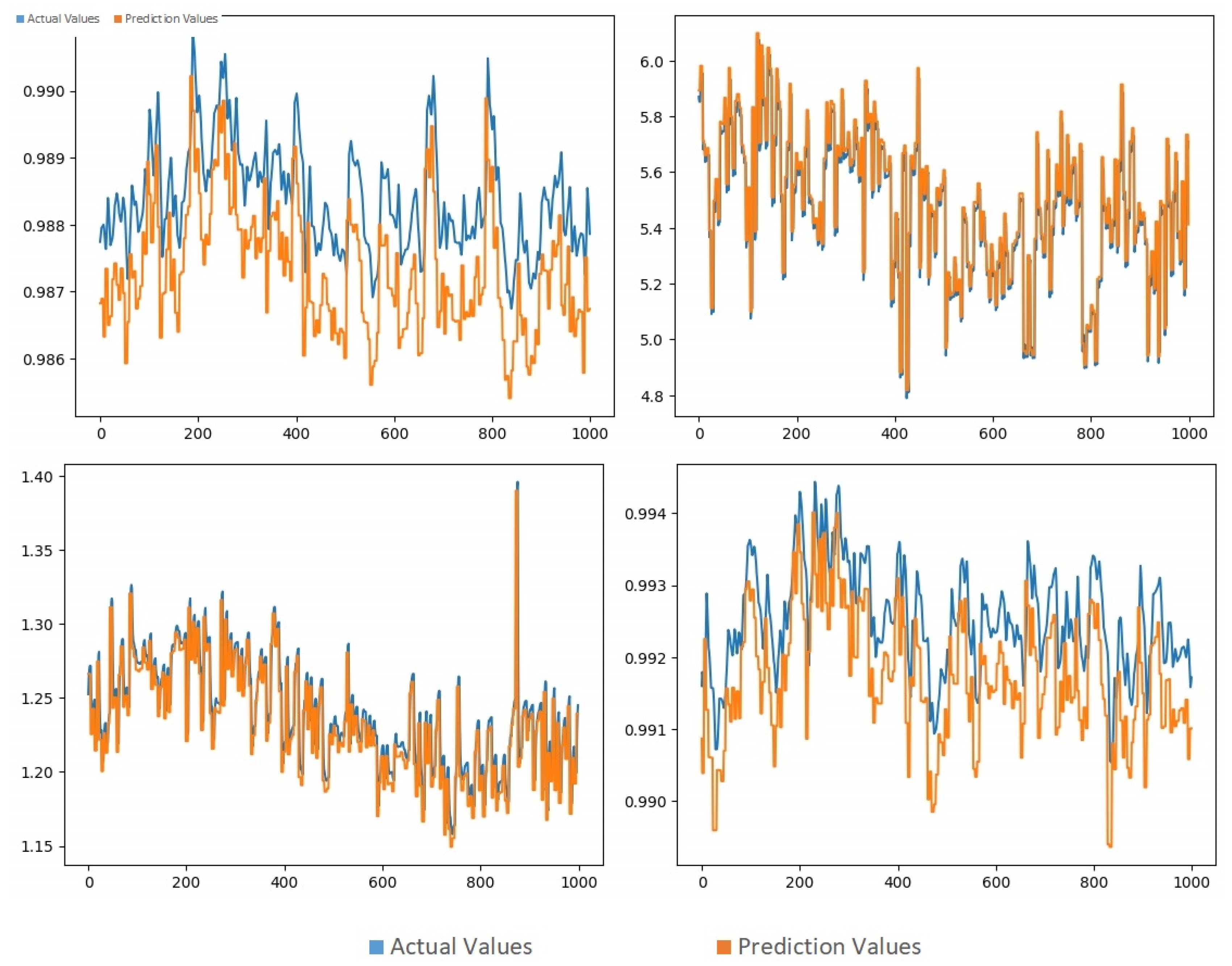
First, in order to determine which parameter will be used in the estimation process, a prediction study was carried out with the vanilla LSTM, which is the basic LSTM method, using four parameters that are important in building energy analysis. These four parameters are total power factor, power factor, Total Harmonic Distortion Voltage, and Total Harmonic Distortion Current. Accordingly, the prediction results can be seen in Figure 1.

The error rate, which measures the quality of the difference between actual values and predicted values, was calculated. As a result, calculations were made using the MAE, MSE, and RMSE error rate methods, which examine the relationship between the prediction results and real data. These error rates are presented in

Table 2. MAE, MSE, and RMSE error rates for different parameters.

Error Rate	TPF	PF	THDV	THDC
MAE	0.00049273	0.00407066	0.01423912	0.06381466
MSE	0.00000045	0.00003065	0.00057725	0.01767848
RMSE	0.00067232	0.00553694	0.02402605	0.13296045

.

In the results obtained, it was observed that the lowest error rate was in the total power factor. Therefore, it was decided to use this parameter in the remaining part and compare the effect of different LSTM methods on TPF estimation.

In the simulations made in this study, some operations were performed to see the advantages of the LSTM method. TPF value is marked as a prediction output. The other 102 variables were marked as an input data set. Specific parts of the data set can be seen in

Table 3. The main data set.

Time	Fundamental Current L1	Fundamental Current L2	Fundamental Current L3	Fundamental Voltage L1 N	…	Voltage L2 L3	Voltage L2 N	Voltage L3 L1	Voltage L3 N
14/03/2023 00:00:00	794.15387	829.668396	847.513855	235.914963	…	407.441772	235.386368	409.844940	236.237823
14/03/2023 00:00:10	794.15387	829.668396	847.513855	235.914963	…	407.441772	235.386368	409.844940	236.237823
14/03/2023 00:00:20	794.15387	826.391541	847.513855	235.914963	…	407.441772	235.386368	409.844940	236.237823
14/03/2023 00:00:30	794.15387	826.391541	847.513855	235.914963	…	407.441772	235.386368	409.419769	235.818710
14/03/2023 00:00:30	794.15387	826.391541	838.068115	236.014099		407.282501	235.618973	409.419769	235.818710
…	…	…	…	…	…	…	…	…	…
11/06/2023 23:59:10	625.857666	647.464722	612.793396	233.746002	…	404.129364	233.418060	406.201691	234.028564
11/06/2023 23:59:20	625.857666	647.464722	612.793396	233.746002	…	404.129364	233.418060	406.201691	234.028564
11/06/2023 23:59:30	625.857666	647.464722	612.793396	233.746002	…	404.129364	233.418060	406.201691	234.028564
11/06/2023 23:59:40	625.857666	647.464722	612.793396	233.746002	…	404.129364	233.418060	406.201691	234.028564
11/06/2023 23:59:50	625.857666	647.464722	612.793396	233.746002	…	404.129364	233.418060	406.201691	234.028564

.

A training study was conducted using the LSTM model using the data set given in Table 3. As a result of the training, the predicted values and actual values were examined comparatively. A summary of these results can be seen in

Table 4. Actual and predicted values.

Actual Values	Vanilla	Stacked	Bidirectional	CNN	Encoder–Decoder
0.989418	0.989703	0.989936	0.989856	0.989017	0.989758
0.989418	0.989789	0.989983	0.989926	0.989048	0.989863
0.989418	0.989888	0.990264	0.989917	0.989163	0.989981
…	…	…	…	…	…
0.992353	0.992545	0.992633	0.992589	0.992106	0.992625
0.992353	0.992535	0.992621	0.992652	0.992058	0.992611
0.992353	0.992521	0.992608	0.992634	0.992073	0.992598

.

In this study, a prediction study was carried out on the data set with five different types of LSTM. These LSTM types are vanilla LSTM, stacked LSTM, bidirectional LSTM, CNN-LSTM, and encoder–decoder LSTM. As can be seen, the differences between the actual values and the predicted values resulting from these LSTM models are extremely low.

In Table 4, the TPF value was estimated using five different types of LSTM. Some of these estimates and actual values are exhibited. The error rate, which measures the quality of the difference between actual values and predicted values, was calculated.

As a result, calculations were made using the MAE, MSE, and RMSE error rate methods, which examine the relationship between the prediction results obtained as a result of each LSTM method and the real data. Data, including error rates, are presented in

Table 5. MAE, MSE, and RMSE error rates for each LSTM method.

Error Rate	Vanilla LSTM	Stacked LSTM	Bidirectional LSTM	CNN-LSTM	Encoder–Decoder LSTM
MAE	0.00049273	0.00050961	0.00058058	0.0005544	0.00054516
MSE	0.00000045	0.00000047	0.00000052	0.00000048	0.00000049
RMSE	0.00067232	0.000685565	0.00072111	0.00069282	0.00070089

.

According to these outputs, vanilla LSTM stands out with its lower error rate compared to other methods. The low error rate of this method has also been seen in all three error rate calculation methods.

So, it can be said that the vanilla LSTM, one of the methods used in this study, stands out as the best LSTM method for this type of data set. While the MAE error rate in the vanilla LSTM method was measured as 0.00049273, it was observed that the error rate was slightly higher in other prediction methods. These error rates can be seen graphically in Figure 2.

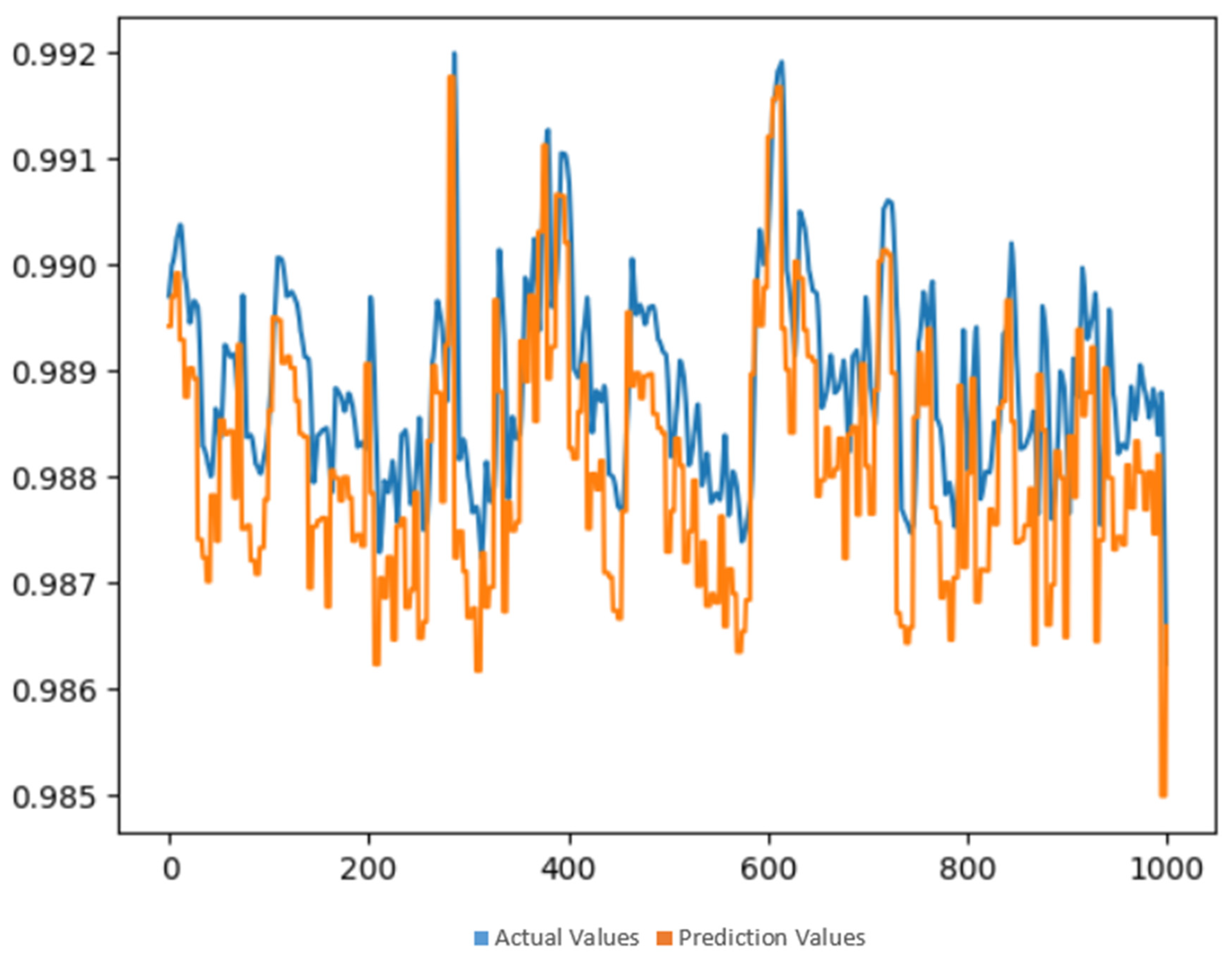
It can be seen from these error rates that the most efficient method to be used for energy analysis in the building subject to our study is vanilla LSTM. The values were plotted in order to better observe the similarity between the results with vanilla LSTM and the actual values. Figure 3 shows the forecasting results of the vanilla LSTM model. In this figure, the TPF change between day and night hours can be clearly seen. At the same time, since the data are very frequent, the actual and estimated lines are mixed together. But this confusion is also an indicator of how close the prediction is to reality.

Figure 4 shows the same results for a slightly narrower time period. In this figure, the closeness between the predicted and actual values of TPF value can be observed. In this study, the error rate was calculated as 0.00049273 with the MAE method.

Based on previous studies, it was deemed appropriate to compare LSTM models for the green building energy analysis process in this article. Additionally, the best LSTM model detected in this study, vanilla LSTM, was compared with other machine learning models. In this comparison, frequently used methods, SVM, Random Forests models, and the vanilla LSTM model were compared. Error rates showing the difference between the real value and the estimated value were calculated. The relevant comparison table can be seen in

Table 6. MAE error rates for Vanilla LSTM, SVM, and Random Forests methods.

Error Rate	Vanilla LSTM	SVM	Random Forests
MAE	0.00049273	0.00126247	0.00389523

. Calculations were made using the MAE error rate method.

Since the building studied in the article is a green building and has many optimization systems, low error rates were calculated for each model, as expected. However, as seen in Table 6, when the relevant data are analyzed with the specified methods, the lowest error rate is still in vanilla LSTM.

The LSTM model is frequently used in time series forecasting. It stands out in detecting long-term time dependencies and performs well with consecutive data. The SVM model is generally suitable for small-to-medium-sized data sets. As data sets become smaller, the accuracy rate increases. However, as the data titles increase, the error rate increases. The Random Forests model is generally used in regression operations. Despite the advantage of being able to work even in cases of missing and incorrect data, the error rate increases like SVM when the data titles increase. In this study, a very high-scale data set was used. A data set consisting of 779,280 rows and 102 columns was used in this study, and as can be seen from the results, the LSTM model obtained more efficient results. In addition, the SVM and Random Forests models again fall behind the LSTM model due to their slow operation in high data sets.

Vanilla LSTM is generally used in simple time series predictions and small sequential data problems. In other words, the complexity of the data set, rather than its size, can be given as an example of the reasons that can lead to errors. Stacked LSTM is preferred in data sets with more than one layer. Complex data sets, such as financial time series prediction and speech recognition, are suitable for this model. In the bidirectional LSTM model, data can be read in two ways. Data evaluation depends on feedback. It is suitable for use in processes where it is necessary to return to previous predictions, such as natural language processing and text classification. The CNN-LSTM model is suitable for visual content data sets, such as video classification and weather forecasting on map data. It can work with noisy data, but the training time is long. The encoder–decoder LSTM model is used for technologies, such as language translation and automatic subtitling. As explained above, each LSTM sub-model has a separate area of use. Among these, the vanilla LSTM is observed as the most suitable model because the data set used in the study is single-layer, and contains a high number of data, but each data cell consists of simple numbers and shows the feature of a time-based data set. The results we obtained in the study also showed that the vanilla LSTM model was suitable for this data set.

4. Conclusions

Hospitals that provide green building features not only have devices that draw high power but also have systems that reduce the effects of these features. Therefore, precise measurement and analysis are extremely important in such buildings. In previous studies, the effects of different LSTM methods on energy analysis along with different machine learning techniques have been examined. The most appropriate analysis method varies depending on whether the place to be studied is a building or a house. When it comes to buildings, different situations, such as whether the building is a public or private building, whether it is a production center or a user center, whether it is crowded or sparse, and the nature of the devices inside, have brought different prediction techniques to the fore. LSTM comes to the fore in buildings that consume high energy. Previous studies have shown that different techniques of LSTM are more suitable for the building being studied. In this study, the LSTM model, which is a sensitive energy analysis method suitable for such structures, was used. The energy data of a hospital were analyzed with five different LSTM models. These are vanilla LSTM, stacked LSTM, bidirectional LSTM, CNN-LSTM, and encoder–decoder LSTM. Different LSTM techniques were applied to different parameters. TPF, which had the lowest error rate among these parameters, was selected as the analysis parameter. In the analysis, the change in TPF value according to days and hours was observed. An estimation study on TPF was also performed through the data set. It has been observed that the prediction and actual results are consistent to a good degree. The effect of five different LSTM models on the results was observed. It was found that the vanilla LSTM model had the highest accuracy and lowest error rate. The error rate was calculated with three different methods. The MAE error rate was calculated as 0.00049273, the MSE error rate was calculated as 0.00000045, and the RMSE error rate was calculated as 0.00067232 for the vanilla LSTM method. With these low error rates obtained, it can be concluded that the vanilla LSTM model is suitable for green buildings with high consumption.

In buildings with high-energy-consuming machines, power factor values deviate from the ideal value due to energy fluctuation. This situation prevents the smooth operation of the electrical system. Different techniques are used in buildings to bring the power factor to values close to ideal. The building in question currently has components, such as energy storage devices and compensation panels, to correct this problem. Although the values obtained in this study are acceptable values, the following operations can be applied to improve the system:

Regional energy analysis can be performed, and local compensation devices can be integrated into the relevant regions for special precautions by determining which units experience density at which hour intervals. Filtering can be performed by considering the total harmonic distortion values. Considering the load diversity of the building in question, it has been observed that an active filtering option is more suitable instead of a simple passive inductor-capacitor filtering. Inductive current values can be balanced by adding power factor correction capacitors and providing regular inspection and preventive maintenance. The energy monitoring system in the building in question receives detailed values only from the main panel and only basic values from regional panels. In order to produce correct solutions according to the regions, there should be an energy analyzer that receives detailed data in each different polyclinic panel in the hospital.

In this study, the focus is on which method is more appropriate rather than the seasonal variability of the data. In the further studies to be conducted consecutively, 18 months of data will be used. In this way, the suitability of the method will be confirmed with a larger data set, and at the same time, the differences and errors created by seasonal changes will be included in the analysis.