Article

Inversion Analysis of Stress Fields Based on the LSTM–Attention Neural Network

1
National Institute of Natural Hazards, Beijing 100085, China
2
School of Civil Engineering, Qingdao University of Technology, Qingdao 266520, China
*
Author to whom correspondence should be addressed.
Appl. Sci. 2025, 15(17), 9567; https://doi.org/10.3390/app15179567
Submission received: 3 July 2025 / Revised: 24 August 2025 / Accepted: 27 August 2025 / Published: 30 August 2025

Abstract

Conventional geostress methods of measurement cannot reveal an accurate geostress field distribution in an engineering area, limited by both cost and prevailing geological conditions. This study introduces an improved LSTM–Attention neural network for in situ stress field inversion. By integrating long short-term memory (LSTM) networks—which capture temporal dependencies in sequential data with attention mechanisms that emphasize critical features, the proposed method addresses inherent non-linearity and discontinuity challenges in deep subsurface stress field inversion. The integrated LSTM and multi-head attention architecture extracts temporal features and weights critical information within ground stress field data. Through iterative refinement via optimizers and loss functions, this framework successfully inverts stress boundary conditions while mitigating overfitting risks. The inversion of the stress field around a hydropower station indicates that the proposed method allows accurate inversion of distribution of the geostress field; the inversion values of the maximum principal stress, intermediate principal stress, and minimum principal stress conform to those measured. This study provides a new method for accurately and reliably inverting the stress field for deep engineering geological surveys and rock mass engineering design, which has significant scientific value and engineering application prospects. The rockburst risk of chambers is evaluated according to the stress field, which shows that locations with a burial depth of 274.3 m are at moderate to weak risk of rockburst.

1. Introduction

The geostress field of deep rock mass exhibits non-linear and discontinuous features due to the influences of factors including the complex geological environment, inhomogeneity, and multi-field coupling effects. They bring challenges to the inversion of geostress fields. Although conventional geostress measurement methods, such as the stress-relief method and hydraulic fracturing method, can provide local geostress data, they fail to reveal accurate geostress field distributions in the areas where engineering works are undertaken, being limited by both cost and the prevailing geological condition [1,2,3]. In recent years, data-driven methods based on numerical simulation and machine learning have gradually matured, providing a new idea for the inversion of geostress fields [4,5,6,7,8]. The inversion methods of geostress fields mainly fall into two types: physical model-based, seismic source mechanisms, and data-driven methods.
The physical model-based methods, including the finite element method and boundary element method, require the establishment of an accurate geological or mechanical model and selection of the appropriate boundary and initial conditions, so as to invert the geo-stress field in the area of interest [9,10,11]. Zhao et al. [12] considered that it is reasonable to use roller boundary conditions for the inversion of geostress fields, and the boundary dimensions of the model should be greater than the excavation affected zone. Liang et al. [13] established a three-dimensional (3-d) geological model of a mining area and employed multiple linear regression (MLR) for inversion of the stress field in the deep coal seams. Zhou et al. [14] developed an MLR-based geostress inversion method with improved boundary conditions to solve the non-linear problem caused by the irregular ground surface. Song et al. [15] proposed a geostress inversion method combining the Rhino precision modeling and horizontal isotropy theory, which is applied to the inversion of stress fields in the Gudishan fault zone.
Employing the source mechanism inversion method, the regional stress field is inverted through stress tensor decomposition, which relies on the solutions of fault planes from numerous earthquakes [16,17,18]. Hardebeck et al. [19] put forward the damped stress tensor inversion method. By constraining the fault slip direction to be consistent with the shear stress, this method remarkably enhances the inversion accuracy. Vavrycuk et al. [20] further developed a stress–fault joint iterative inversion framework. For the first time, this framework realizes the simultaneous optimization of stress principal axes and fault geometry, thus resolving the coupling problem between stress and faults in traditional stress field inversion. Schliwa et al. [21] used seismic source mechanisms in combination with seismic and geodetic data for dynamic stress field inversion, uncovering the intricate interaction between co-seismic and post-seismic fault activity.
Data-driven methods, such as the artificial neural network and support vector machine, can effectively process non-linear data and accurately reflect the non-linear and discontinuous features of regional stress fields [22,23,24]. Li et al. [25] analyzed the geostress distribution in Xiluodu using a genetic algorithm-BP neural network, combined with the measured geostress data, and found that the depth exerts the greatest influence on the maximum horizontal stress. Fu et al. [26] built a 3-d numerical model for the Segrila region and determined the distribution of regional stress fields utilizing the support vector regression (SVR) method. Song et al. [27] came up with an inversion method of stress fields based on long short-term memory network (LSTM)-mixed optimization algorithm, which solves the non-uniqueness of boundary conditions in the inversion of stress fields. Zhou et al. [28] addressed the non-linearity, discreteness, and noise in data through optimal learning of time series and inverted the stress field distribution in the Shanghaimiao mining area in the Inner Mongolia Autonomous Region, China.
The ZK65 rock stress field is affected by geological heterogeneity, multi-field coupling effects, and terrain undulations, exhibiting strong non-linearity and spatial discontinuity. Traditional physical-model-based inversion methods, such as the finite element method, depend on precise boundary condition settings and exhibit low computational accuracy. Seismic-source-mechanism-based methods can only impose constraints on the stress direction and relative magnitude, failing to yield absolute stress values, which restricts their practical engineering applications. Conventional data-driven approaches, specifically traditional neural networks, possess limited capabilities in capturing long-term data dependency features and are susceptible to the noise in training data. To address the above issues, this study puts forward a hybrid model that combines long short-term memory networks (LSTM) with attention mechanisms (Attention). The objective is to leverage the gating mechanism of LSTM to capture the temporal dependencies within the deep-seated ground stress field sequences. By means of attention weights, the representational capabilities of sensitive regions, including fault zones and high-stress gradient zones, can be dynamically enhanced, while irrelevant noise can be suppressed, thereby improving the inversion accuracy of the ground stress field.

2. Inversion of the Non-Linear Geostress Field

2.1. Basic Procedure of Inversion

The inversion of geostress fields is classified as an optimal approximation problem [28], and it is thus addressed as the following: (1) Different loading conditions of stress (or displacement) are applied to each boundary of a finite element model to form a subspace generated by stress data, demarcate stress distribution ranges of different types of faults in the research region, and determine the reasonable computation condition. (2) Then, the stress data under computation conditions are integrated with the measured ones to form a subset space of the Hibert space.
If the dimension of the subspace of measured data is lower than that of the calculated stress, the stress field can be inverted through use of MLR or a genetic algorithm. However, due to the high dimension and strong non-linear characteristics of deep geostress data [29,30], the dimension of its subspace is generally higher than that of the calculated stress, which renders the inversion more difficult. To solve the problem, an inversion method of geostress fields on the basis of the LSTM–Attention neural network algorithm was proposed to improve the inversion accuracy by dimension reduction of the sample subspace and deep optimization of the basis subspace (subspace of calculated stress). The process is illustrated in Figure 1.
The specific implementation process is as follows:
(1) Construction of the finite element model: based on the actual measurement data from the engineering site, the stress boundary range of the model is initially determined, and multiple sets of random stress boundary conditions are generated.
(2) Definition of stress fields in discontinuous structural zones: Finite element calculations are carried out to determine the stress fields under various operating conditions, and the rationality of the stress distribution in fault zones is verified. If the requirements are not met, the boundary conditions are readjusted.
(3) Acquisition of in situ stress data: in situ stress data are collected from the site and divided into training and testing datasets for neural network training and validation.
(4) Training of the neural network model: The stress values at measurement points under different operating conditions are used as the input data for training samples, and the stress field distributions are used as the output data for training samples. Then, the model is trained using the LSTM–Attention neural network algorithm.
(5) Testing and validation of the model: the error metrics between the inverted stress and the measured stress are calculated, and the prediction accuracy of the model is compared and analyzed to validate its reliability.
(6) Application of the model: regional rockburst risks are evaluated based on the tangential stress criterion and engineering standards.

2.2. LSTM–Attention Neural Network Algorithm
The LSTM–Attention neural network algorithm is a deep learning model that combines Short-Term Memory and the Attention Mechanism [29,30,31]. Therein, LSTM can effectively capture the long-term dependency in the time-series data, and Attention Mechanism enhances the ability of the model to focus on salient features by dynamically weighting the input information. The combination of the two is applicable to process complex data with the long-range dependence and non-linear features.
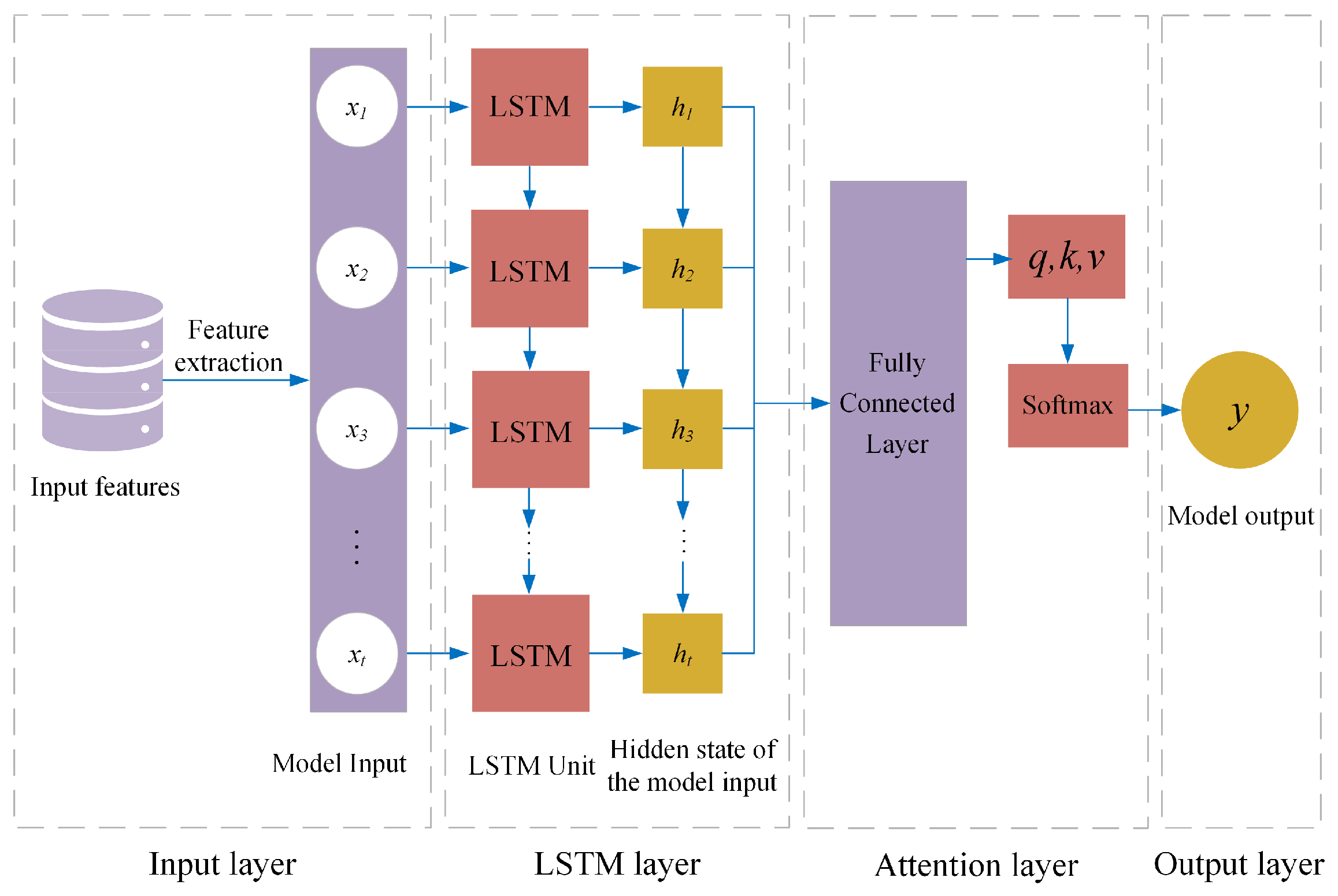
The structure of the LSTM–Attention model (Figure 2) mainly includes three parts: (1) the LSTM layer: this is used to extract sequential features of the input sequences and generate hidden state sequences; (2) the attention layer: the attention weight is calculated based on the hidden states of LSTM and the multi-head attention output is generated; (3) the output layer: the output format of multi-head attention is matched with the distribution format of stress fields to generate the final output. The specific process is described as follows:
(1) The input sequences pass through the LSTM layer, the structure of which mainly includes a forget gate, an input gate, updating of cell states, an output gate, and updating of hidden states.
The forget gate determines what information should be discarded by elements in the neural network and is expressed as
f t = σ W f h t 1 ,   x t + b f
where f t is the output of the forget gate at time moment t ; σ is an Sigmoid function; W f is the weight matrix of the forget gate; h t 1 is the hidden state at the previous time; x t is the input at the current time; and b f is the offset of the forget gate.
The input gate determines what information is stored in elements of the neural network, which consists of the input gating signal and the candidate cell state. The input gating signal is expressed as
i t = σ W i h t 1 ,   x t + b i      
where i t is the input gating signal at time moment t ; W i is the weight matrix of the input gate; and b i is the offset of the input gate.
Figure 2. Diagram of the LSTM–Attention neural network structure.
Applsci 15 09567 g002
The candidate cell states are given by Equation (3):
C ~ t = t a n h W c h t 1 ,   x t + b c      
where C ~ t is the state of candidate elements in the neural network at time t ; W c is the weight matrix for calculating the state of candidate elements in the neural network; b c is the offset; and tanh is the hyperbolic tangent function.
The cell states are updated according to the output of the forget and input gates and is expressed as
C t = f t C t 1 + i t C ~ t      
where C t is the cell state at time t after updating; d is the cell state at the previous time; and represents the element-level multiplication.
The output gate controls what information in elements of the neural network serves as the output at the current time as per Equation (5):
o t = σ W o h t 1 ,   x t + b o
where o t is the output of the output gate at time t ; W o is the weight matrix of the output gate; and b o is the offset of the output gate. The hidden state is updated.
The hidden state h t at the current time is calculated according to the output gate and the updated cell state and is expressed as
h t = o t t a n h C t  
(2) The output data of the LSTM output layer enter the attention layer. Firstly, three parallel fully connected layers are adopted to calculate the query (Q), key (K), and value (V), and their linear transformation results are divided into multiple heads, each of which performs attention computation independently.
(3) The attention weight of each head is computed using the scaled dot-product attention.
(4) The attention weight of each head is normalized based on the Softmax function. In this way, the weight can be explained as the probability distribution.
(5) The normalized attention weight is adopted for weighted summation of V, thus obtaining the output of each head and is expressed as
A t t e n t i o n ( Q i , K i , V i ) = s o f t m a x ( Q i K i T d k ) V i
where Q is utilized to calculate the attention score; K is used to compare with Q; and V is multiplied by the attention weight to produce the final output. Q, K, and V are obtained via linear transformation of the self-attention score layer below; i is the ith attention head in the multi-head self-attention mechanism.
The fully connected layers are adopted to match the output format of the attention layer with the distribution format of stress fields, thus generating the final output as per Equation (8):
Q i = X W Q i K i = X W K i   V i = X W V i
where X is the input tensor on the self-attention score layer and W Q i , W K i ,   a n d   W V i are trainable parameter matrices.
After extensive training and debugging, the model parameters were finalized as follows: initial learning rate of 0.0001, three LSTM layers, 512 hidden units, sequence length of 10, eight attention heads, and 1000 training iterations. The integration of LSTM with multi-head attention enables temporal feature extraction and weighted key-information selection from ground stress field data. The model was iteratively refined using an optimizer and loss function, with L2 regularization introduced to mitigate overfitting. After 1000 training iterations, the loss converged progressively, demonstrating robust generalization on the test set. The model successfully inverted stress boundary conditions, confirming the efficacy of combining data-driven methods with physical constraints.

3. Calculation of Geostress Around a Hydropower Station

3.1. Overview of Engineering Geology

The hydropower station is located in Yarkand River valley, where the elevation is 2400 m (above mean sea level), while the elevation of the mountain crests on both sides of the valley is 4000 to 5000 m. A canyon landform is formed in the region due to crustal arching and river incision, which can be divided into three geomorphic units, namely, an alpine region, a medium-high mountain area, and a low-mountain and hilly area.
The alpine region is west of the Miya fault and has an elevation of 3500 to 6000 m, with complex terrain. Due to the strong river incision, the relative altitude difference exceeds 1000 m, the river is twisting with a longitudinal slope of 3‰ to 5‰, and the river valley is either U- or V-shaped. The medium-high mountain area is situated between the Miya fault and Aertashi fault at an elevation of 2500 to 3500 m, where the river valley is mainly U-shaped and has a bottom width of 250 to 450 m. The low-mountain and hilly area is east of the Aertashi fault and generally lower than 2500 m, with river valleys being 550 to 3500 m wide and with a rugged topography.
The outcrop strata at the power generation and water diversion system mainly include the Carboniferous system, Proterozoic strata, and Quaternary system. The Proterozoic Bulunkuole Group, mainly containing quartz schist and quartz-granulite, is medium-thick layered and has intact structures. The Carboniferous system mainly consists of sandstone, tuff sandstone, and conglomerate, and shows NW-trending zonal distribution. The Quaternary system is widely distributed and includes glacial drift, proluvial, colluvial slope, and alluviation.
The strata along the generator chamber show stable occurrence, with a strike angle of 320° to 350° SW and an included angle of 30° to 50° with the chamber axis. There is no large fault along the generator chamber, while small faults are developed, and the included angle between most faults and the chamber axis is greater than 30°. The occurrence of main faults is described in Table 1.

3.2. Computational Model

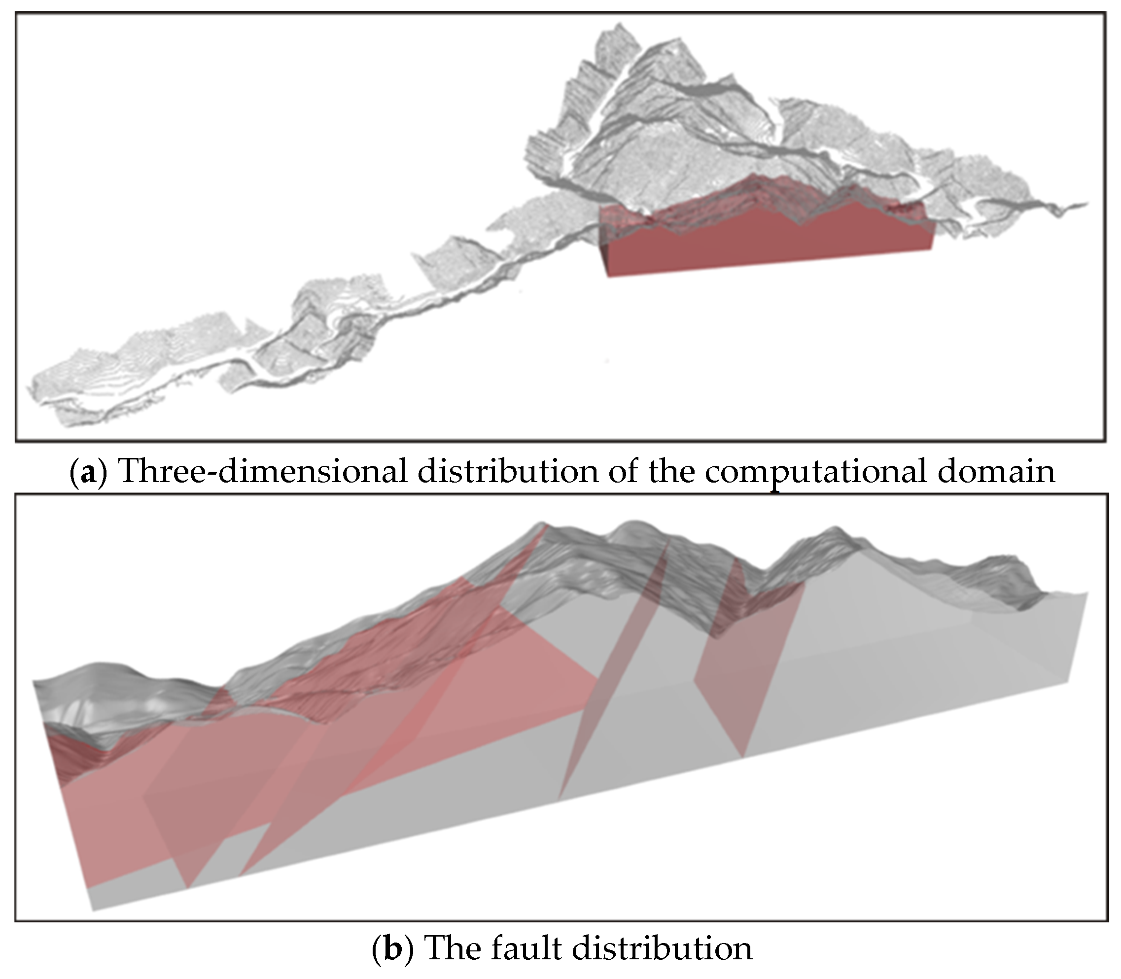
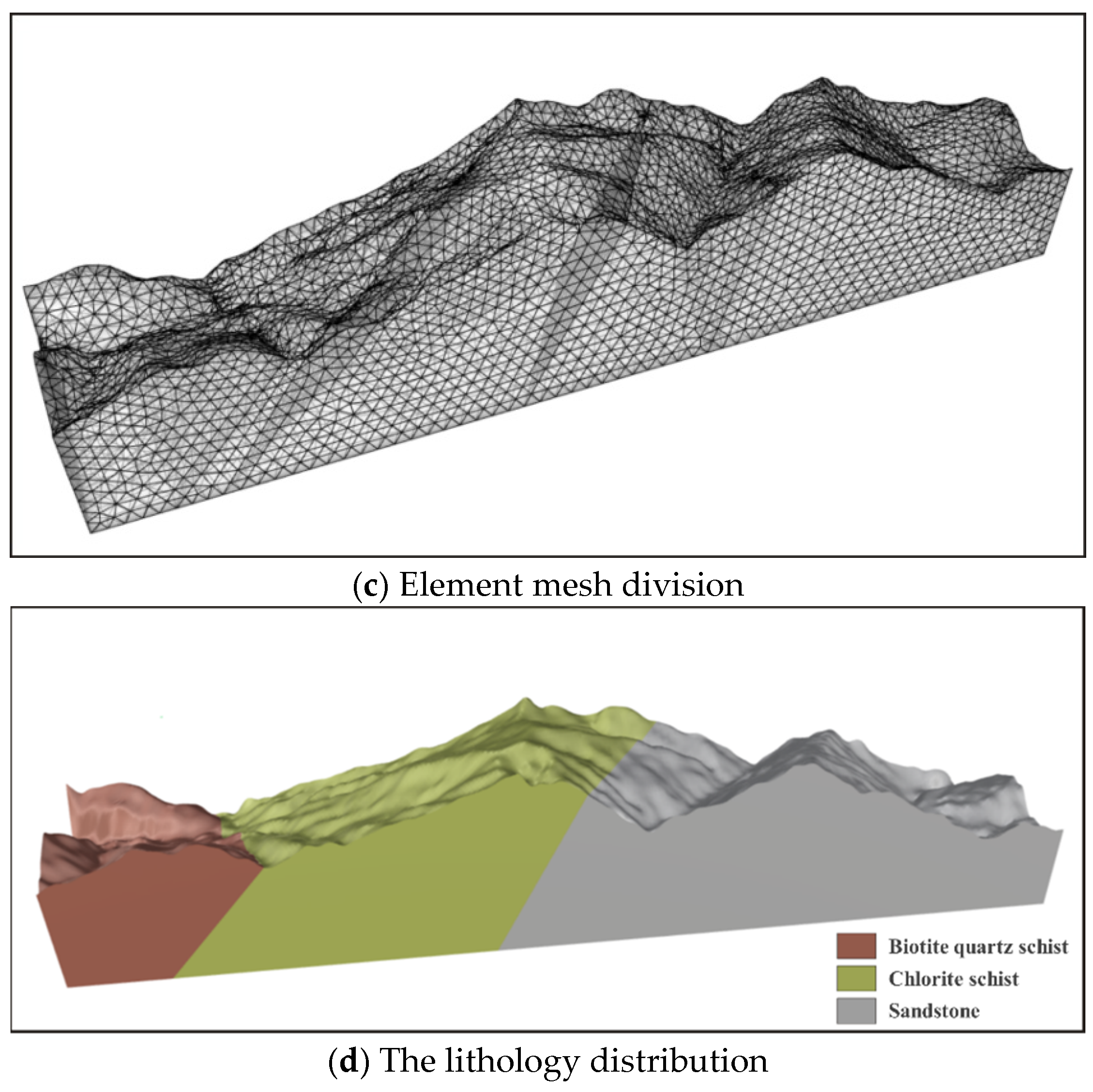
Two principles should be followed to determine the computational domain: (1) The geometric range should completely cover the engineering affected zone and be appropriately enlarged to reduce the boundary effect. (2) The geometric constraints at the boundary should be easy to determine [31]. Based on the range of the engineering area and the engineering geological condition, the computational domain is ascertained to be a rectangular plane domain with a long axis of 12,320 m and a short axis of 2060 m, as shown in Figure 3a. The powerhouse chamber is 600 to 1000 m from the fault zone, where secondary faults and joint fissures are relatively well developed. NNW and NNE-trending faults are mainly developed along the chamber. According to statistical results pertaining to such faults (Table 1), representative faults are taken for geostress simulation. The fault distribution is illustrated in Figure 3b. Through finite element mesh division, 121,130 elements and 59,843 nodes are generated, as displayed in Figure 3c. The lithological distribution in the computational domain is displayed in Figure 3d. Mechanical parameters of rock masses and faults are listed in Table 2 and Table 3.

3.3. Geostress Measurement Results

The hydraulic fracturing method was utilized to measure the geostress in ZK59, ZK60, and ZK65 boreholes, and the results are shown in Table 4.

4. Inversion of the Geostress Field

4.1. Inversion Process of the Geostress Field

4.1.1. Boundary Conditions of the Model

The vertical displacement on the bottom of the model was fixed, the upper ground was set as a free face, and the normal constraint was applied to the side face. On the basis of the measured geostress data, 10 groups of boundary conditions of uniformly distributed compressive stress and linearly increasing compressive stress were applied to different side faces (Table 5). All of the 10 groups of working conditions should meet the demarcation range of the stress field of faults [32].

4.1.2. Data Preprocessing

To enhance the training efficiency and generalization capability of the LSTM–Attention hybrid model, this study utilizes 42 sets of in situ stress field measurements. Each dataset contains three principal stress components (σ1: maximum, σ2: intermediate, and σ3: minimum principal stresses) recorded at ten distinct spatial locations. The preprocessing workflow comprises three sequential operations: initial independent normalization of each stress component to the [0, 1] range to eliminate scale discrepancies; subsequent extraction and separate normalization of boundary condition parameters including stress boundaries and gravitational acceleration; and finally, partitioning of the geostress data into training (first 70%) and test sets (remaining 30%). The model accepts measured stress values under various operational conditions as input and predicts the full-field stress distribution as output.

4.1.3. Training of the LSTM–Attention Neural Network

The stress values at measuring points under the 10 groups of conditions were taken as the input of training samples and the stress field distribution as the output of training samples, and they were input in the LSTM–Attention neural network. After extensive training and debugging, the model parameters were finalized as follows: initial learning rate of 0.0001, three LSTM layers, 512 hidden units, sequence length of 10, eight attention heads, and 1000 training iterations. The software environment uses the Python 3.10 programming language and runs the code on a computer equipped with an NVIDIA graphics card and at least 8 GB of graphics memory. The integration of LSTM with multi-head attention enables temporal feature extraction and weighted key-information selection from ground stress field data. The model was iteratively refined using an optimizer and loss function, with L2 regularization introduced to mitigate overfitting. After 1000 training iterations, the loss converged progressively, demonstrating robust generalization on the test set. The model successfully inverted stress boundary conditions, confirming the efficacy of combining data-driven methods with physical constraints.

4.1.4. Calculation and Optimization of the Measured Stress Field

Stress values at the measuring points were input in the optimized LSTM–Attention neural network algorithm, and the output reflects the distribution results of the actual stress field. The acceleration due to gravity was set to 9.732 ms−2. The optimal parameters were substituted into the LSTM–Attention neural network model to determine the distribution of the regional stress field as per Equation (9).
σ ^ Z Z = 7.7974 σ Z Z 1 23.3690 σ Z Z 2 224.6427 σ Z Z 3 22.3742 σ ^ XX = 2.5526 σ X X 1 + 1.5534 σ X X 2 0.9874 σ X X 3 17.6342 σ ^ Y Y = 15.8782 σ Y Y 1 1.2374 σ Y Y 2 6.6738 σ Y Y 3 58.1958
where σ ^ Z Z , σ ^ XX , and σ ^ Y Y are regression values of geostress components in three directions; σ Z Z 1 , σ X X 1 , and σ Y Y 1 are geostress components in three directions under gravity; σ Z Z 2 , σ X X 2 , and σ Y Y 2 are geostress components in three directions under compressional tectonics in the X-direction; σ Z Z 3 , σ X X 3 , and σ Y Y 3 are geostress components in three directions under compressional tectonics in the Y-direction, respectively.

4.2. Geostress Inversion Results

4.2.1. Comparison of Inversion and Measured Values of Geostress

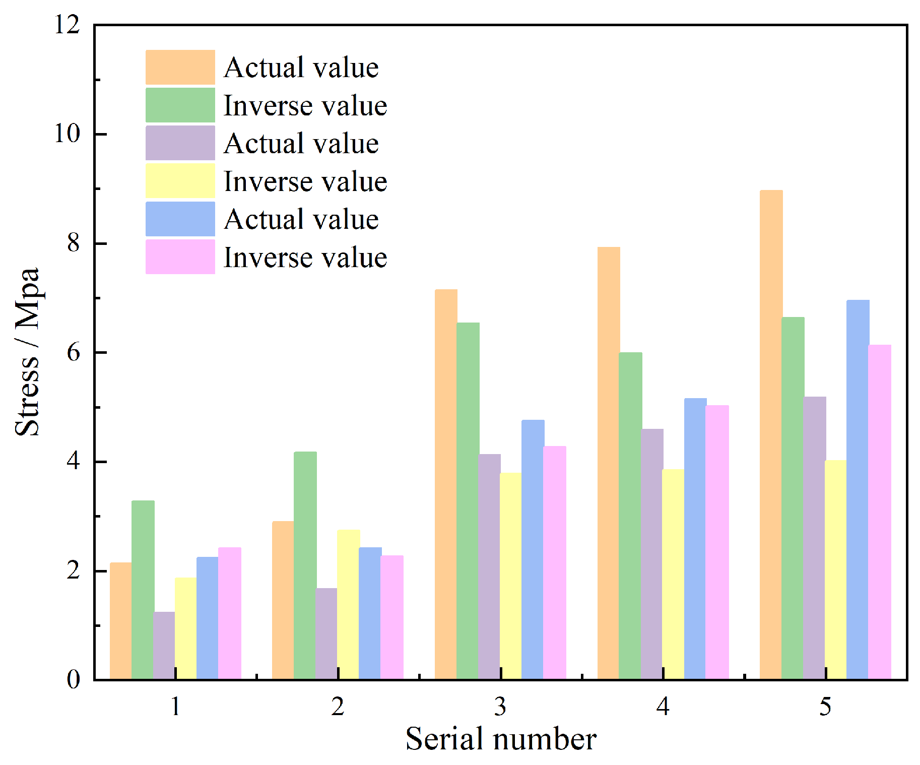
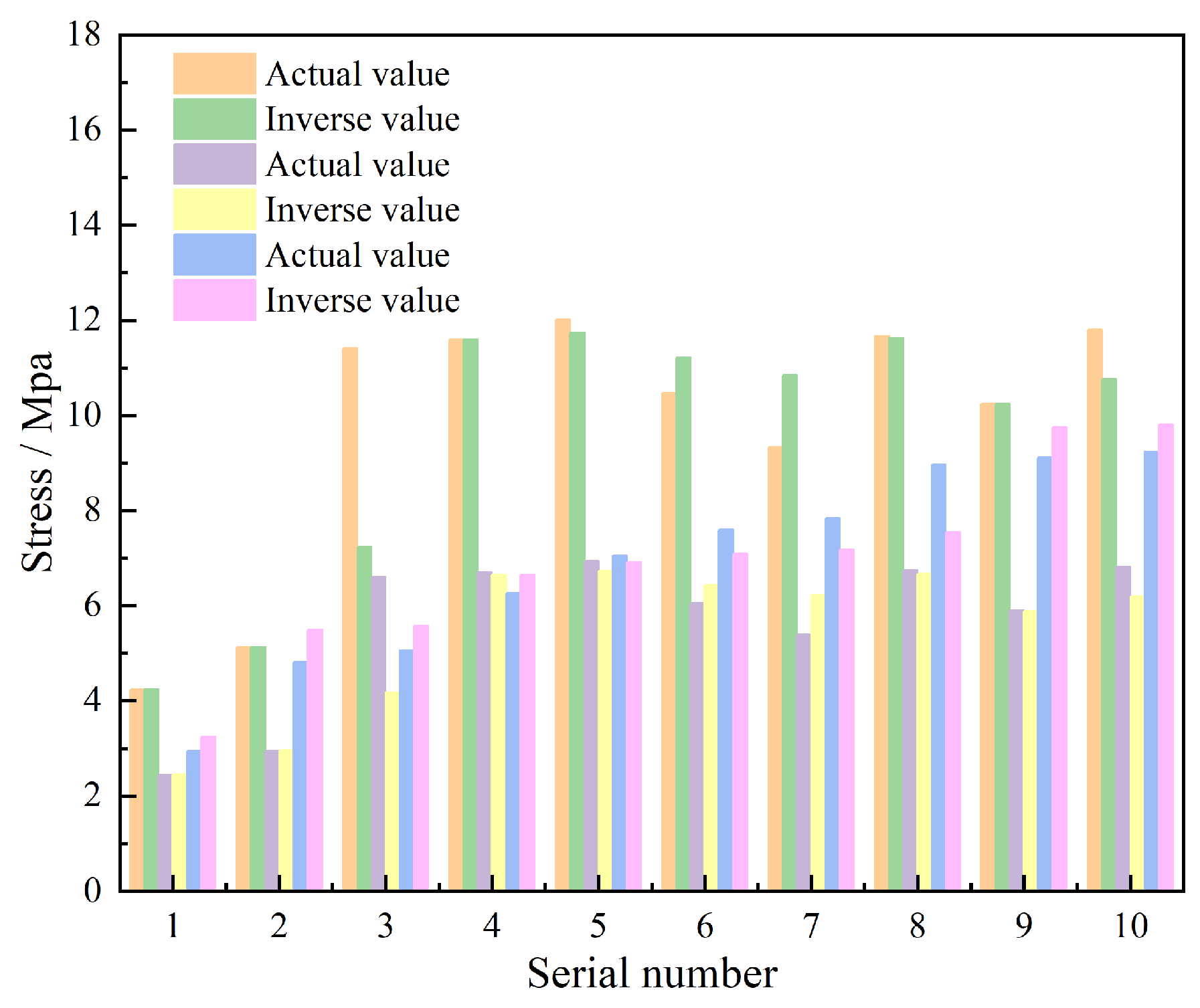
Table 6 and Figure 4, Figure 5 and Figure 6 list inversion and measured values of geostress components in the ZK59, ZK60, and ZK65 boreholes. The inversion values of geostress at the measuring points highly agree with the measured values, and the average errors of the maximum principal stress, intermediate principal stress, and minimum principal stress are separately 0.45 MPa, 0.29 MPa, and 0.23 MPa, indicative of a high inversion accuracy and reliable results.
The calculation results suggest that the inversion errors of the model’s stress field vary with depth. Specifically, the inversion errors in the shallow stress field are relatively large, whereas those in the deep stress field are relatively small. This discrepancy might be attributed to the inadequate consideration of surface unloading, the anisotropy of weathered rock masses, and the effects of groundwater permeability. Additionally, the geological structures corresponding to different boreholes also differ, which results in variations in the stress-field inversion errors of the model. In particular, the stress-field inversion errors are larger in the vicinity of fault zones and smaller in intact rock areas.
The comparison between measured values and inverted values is shown in Table 7. Table 7 indicates that the root mean square error (RMSE), mean absolute percentage error (MAPE), and mean absolute error (MAE) for the maximum principal stress, intermediate principal stress, and minimum principal stress are all close to 0, and the correlation coefficient R2 is above 0.88. The comparison of inversion accuracy for different principal stresses shows that the minimum principal stress > intermediate principal stress > maximum principal stress, further verifying the reliability of the model.

4.2.2. Model Robustness Analysis

The robustness of the proposed model was evaluated by conducting outlier injection tests on the input parameters. The calculation results are shown in Table 8. As the proportion of outliers rises, the model’s inversion accuracy exhibits a declining trend. By setting varying proportions of outliers to be injected into the input parameters, we evaluate the model’s sensitivity to outliers. The findings indicate that the inclusion of outliers leads to a marginal decrease in the model’s inversion accuracy. However, the overall inversion accuracy remains satisfactory, suggesting that the model possesses good robustness.

4.2.3. Comparison and Analysis of Other Models

To verify the reliability of the model presented in this paper, inversion calculations were performed using SVR, MLR, and GA-BP models, respectively. The calculation results are shown in Table 9. The results indicate that the inversion accuracy of the SVR, MLR, and GA-BP models is significantly lower than that of the model presented in this paper, verifying the reliability of the model presented in this paper.

4.2.4. Distribution of the Regional Stress Field

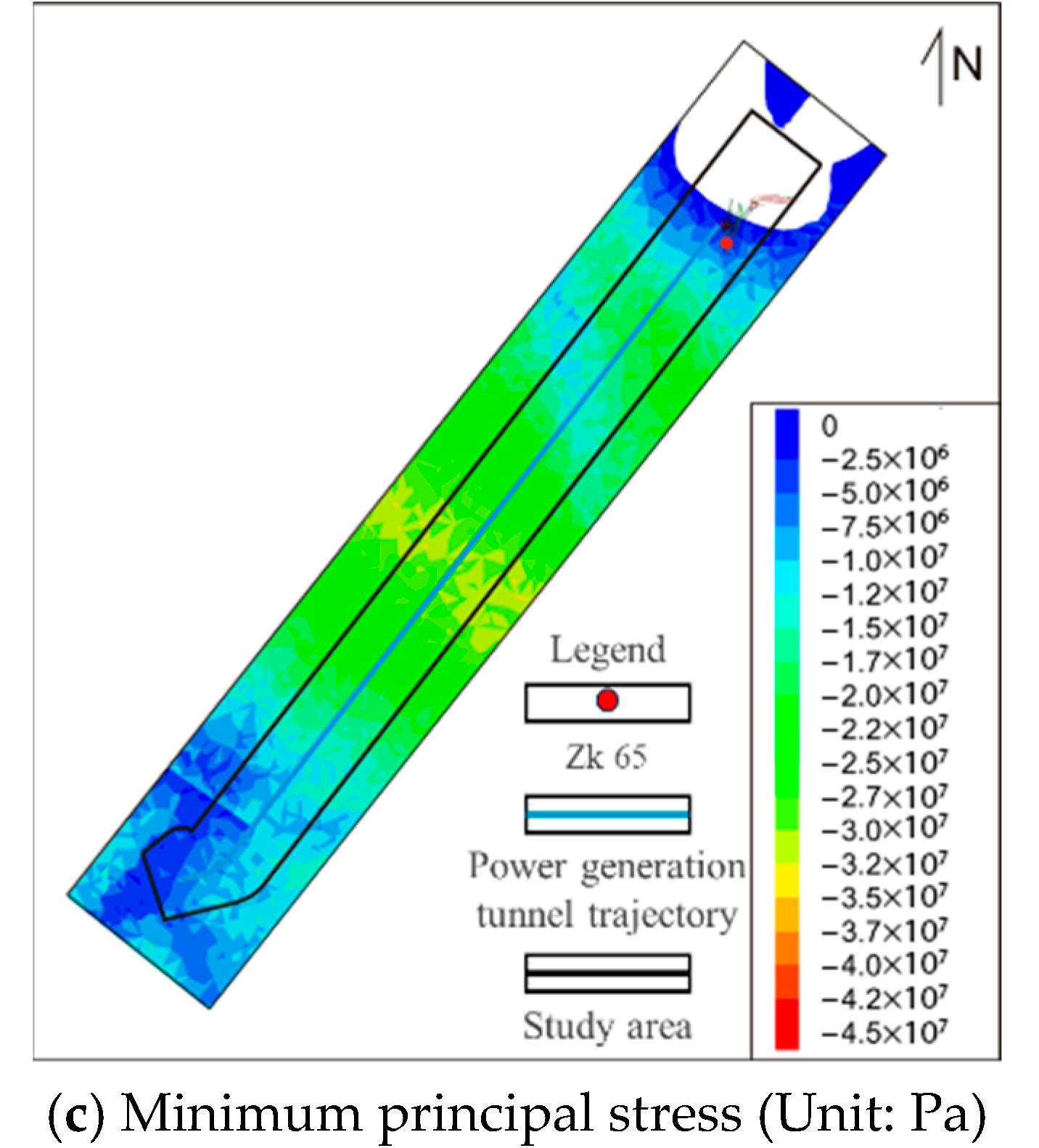
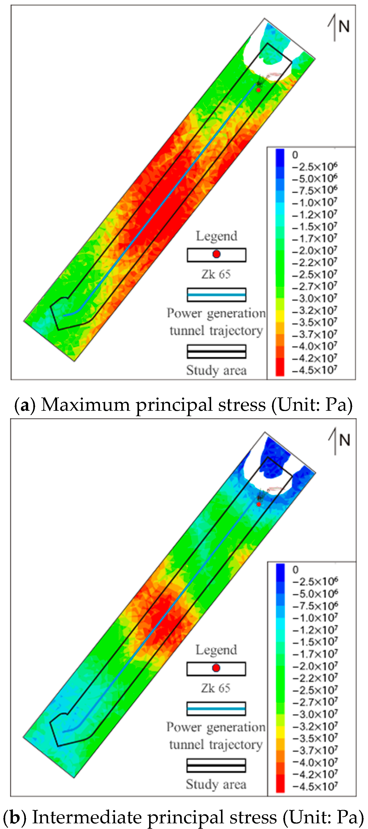
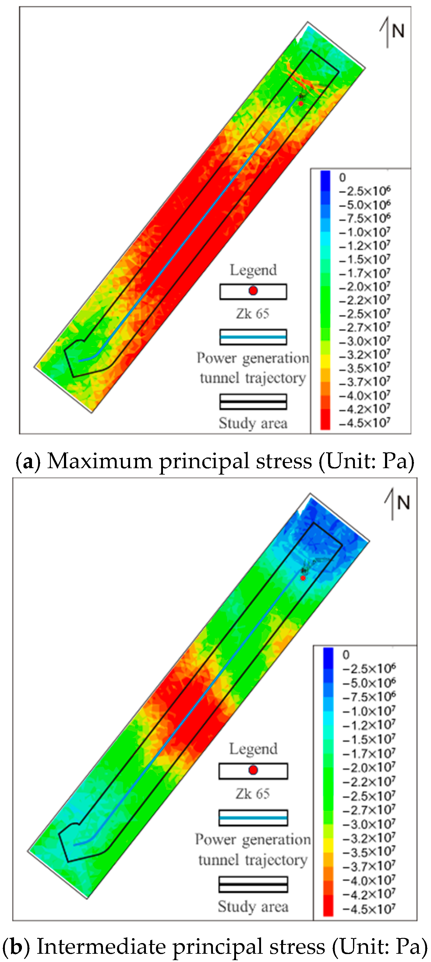
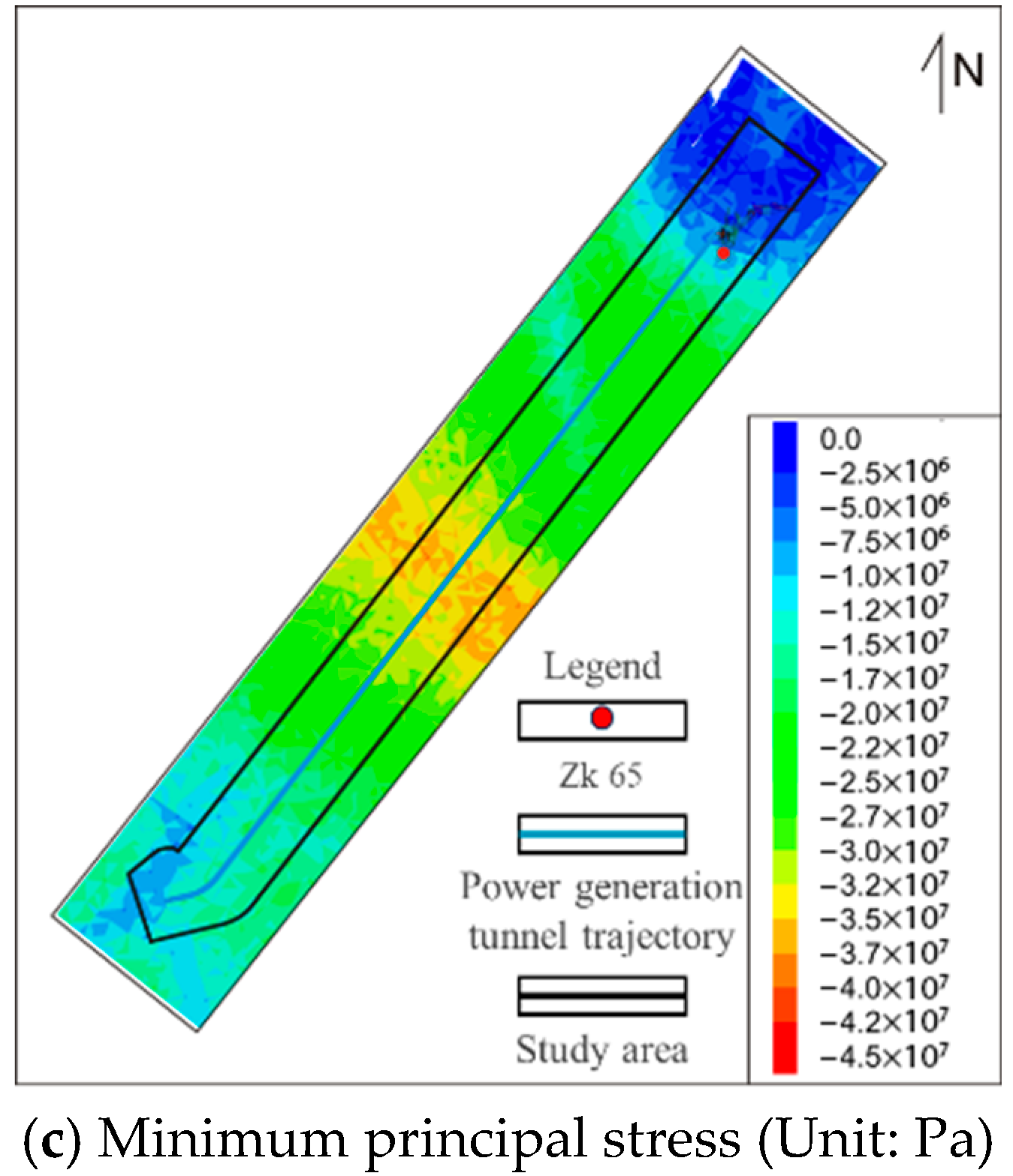
The features of the stress field on the regional horizontal profile were analyzed based on the numerical simulation results, as displayed in Figure 7, Figure 8 and Figure 9. At depths of 100, 200, and 300 m, the maximum principal stress σ 1 , intermediate principal stress σ 2 , and minimum principal stress σ 3 all increase with depth. The maximum principal stress σ 1 is between 5.86 and 39.67 MPa, 11.09 and 47.8 MPa, and 14.60 and 50.18 MPa at depths of 100 m, 200 m, and 300 m; these are 27.19, 31.46, and 34.01 MPa on average. The azimuth of σ 1 remains relatively stable at different depths: it is between N8° E and N15° E, N7° E and N14° E, and N 5° E and N11° E at depths of 100 m, 200 m, and 300 m, respectively. With the increase in the depth, the intermediate principal stress σ 2 and minimum principal stress σ 3 augment, and the azimuth of minimum principal stress σ 3 varies at a depth of 200 m between directions at N28° E to N43° E. The stress gradient is enhanced with the increasing depth, indicative of the complex stress state in deep strata.
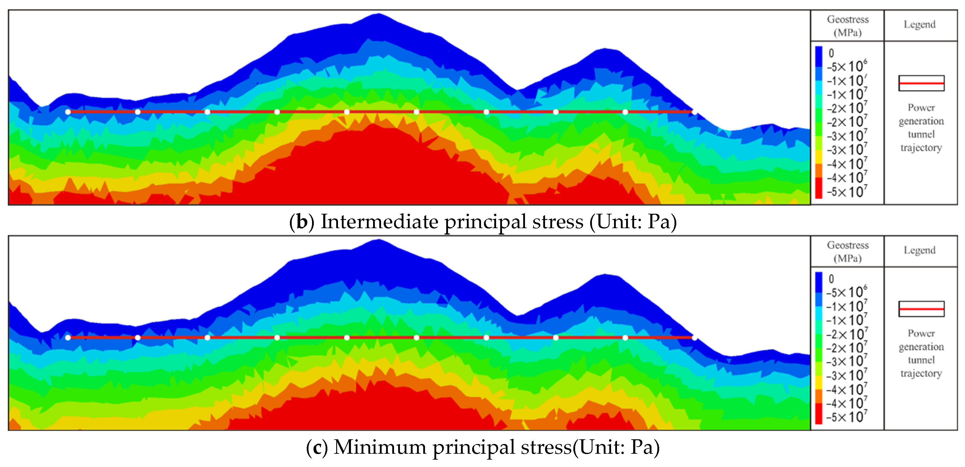
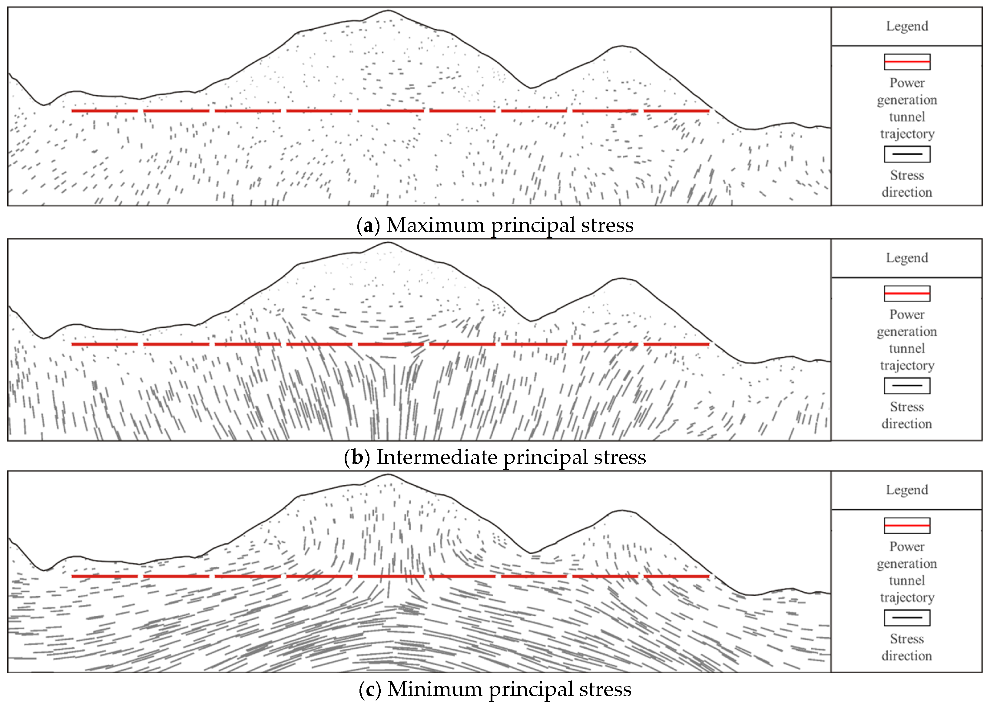
The features of the geostress field on the regional vertical profile are shown in Figure 10 and Figure 11. The maximum principal stress σ 1 , intermediate principal stress σ 2 , and minimum principal stress σ 3 are in ranges of 12.42 to 38.83 (26.11 on average), 5.74 to 34.94 (17.9 on average), and 2.17 to 25.02 (13.55 on average), respectively. The distribution of regional vertical principal stress is significantly affected by the topographic effect, which is shown as a high geostress value in regions of thick overlying strata. On the whole, the vertical geostress field presents characteristics of significant non-linearity in its distribution with stresses fluctuating significantly with changes in the depth and terrain.

4.3. Rockburst Risk Analysis

The rockburst features a complex formation mechanism, and it is mainly influenced by the physico-mechanical properties of rocks (intrinsic factors) and the stress state in the surrounding rocks (external conditions) [33,34,35]. The risk of regional rockbursts is evaluated following the tangential stress criterion [36] and the Standard for engineering classification of rock masses [37].
The segment of the chamber at a burial depth of 274.3 m is studied, and the data pertaining to the principal stress in three directions are shown in Table 6. The chamber axis is along the N38° E-direction, and the dominant direction of geostress is N1° W, that is, the two have an included angle of 39°. The angle α between the plane vertical to the tunnel axis and the direction of the maximum horizontal principal stress is 51°.
The chamber has a circular cross-section. In accordance with classical elastic mechanics, the normal stress on the plane vertical to the chamber axis is
σ H = S H + S h 2 + S H S h 2 cos 2 α
The average values of maximum saturated uniaxial compressive strengths and minimum saturated uniaxial compressive strengths were measured in borehole ZK65, thus revealing the saturated uniaxial compressive strength of the rock to be 73 MPa. Given a measured bulk density of rocks to be 2679 kg/m−3, the maximum initial stress, maximum tangential stress, and their ratio were calculated (Table 10). According to the tangential stress criterion and the Standard for engineering classification of rock masses, the stress state in the region of interest meets the stress conditions for the occurrence of moderate to weak rockbursts, that is, the location at a depth of 274.3 m is at a moderate to weak risk of rockbursts. To address this issue, stress concentration can be reduced through partitioned and layered excavation and the use of pressure-relief holes (Table 11), thereby effectively mitigating the risk of rockbursts.

5. Conclusions

(1) A neural network that integrates LSTM and the multi-head attention mechanism was proposed. The memory ability of LSTM was used to record salient features of the geostress distribution, and the attention mechanism was adopted to screen such features. This increases the number of parameters used in the single LSTM network and alleviates vanishing gradient and gradient explosion that are likely to occur in the cyclic neural network. The proposed neural network also solves the non-linearity and discontinuousness of deep geostress fields and significantly improves the inversion accuracy of geostress field data.
(2) The three-dimensional inversion of the initial stress field around the power generation tunnel at the upstream dam site of the Sangpile Hydropower Station reveals the following findings: A comparison between the measured stress values from boreholes ZK65, ZK59, and ZK60 and the inverted values demonstrates a high degree of consistency, confirming the reliability of the inversion results. Furthermore, the in situ stress field in the engineering area is predominantly governed by self-weight and topographical features. Specifically, in areas with thicker overlying strata, the in situ stress values exhibit an increase, accompanied by variations in the direction of the principal stress.
(3) Based on the results of in situ stress inversion, the risk of rockbursts in the chamber was quantitatively evaluated using the tangential stress criterion and the Engineering Rock Mass Classification Standard. The region at a depth of 274.3 m is found to be at a moderate-to-weak risk of rockburst, providing a new method for comprehensively assessing and managing rockburst risks.
(4) Future work will focus on applying the in situ stress field model presented in this study to structurally complex geological settings, including seismically active regions and deep mining environments, to evaluate its robustness and generalization capacity. Additionally, we aim to integrate multi-physics datasets to improve its capacity for modeling coupled processes under extreme conditions.

Author Contributions

Conceptualization, J.W. and L.Z.; writing—original draft preparation, J.W. and L.Z.; writing—review and editing, J.S. and L.Z.; visualization, J.W. and L.Z. All authors have read and agreed to the published version of the manuscript.

Funding

This research received no external funding.

Data Availability Statement

Data are available from the corresponding author by request.

Conflicts of Interest

The authors declare no conflicts of interest.

References

  1. Han, Z.Q.; Wang, C.Y.; Wang, Y.T.; Wang, C. Borehole cross-sectional shape analysis under in situ stress. Int. J. Geomech. 2020, 20, 04020045. [Google Scholar] [CrossRef]
  2. Lakirouhani, A.; Detournay, E.; Bunger, A.P. A reassessment of in situ stress determination by hydraulic fracturing. Geophys. J. Int. 2016, 205, 1859–1873. [Google Scholar] [CrossRef]
  3. Huang, J.S.; Griffiths, D.V.; Wong, S.-W. In situ stress determination from inversion of hydraulic fracturing data. Int. J. Rock Mech. Min. Sci. 2011, 48, 476–481. [Google Scholar] [CrossRef]
  4. Zhang, L.M.; Zhang, D.; Cong, Y.; Wang, Z.Q.; Wang, X.S. Constructing a three-dimensional creep model for rocks and soils based on memory-dependent derivatives: A theoretical and experimental study. Comput. Geotech. 2023, 159, 105366. [Google Scholar] [CrossRef]
  5. Li, F.; Zhou, J.X.; Wang, J.A. Nonlinear in-situ stress construction method for deep multi-field coupling effects. J. China Coal Soc. 2021, 46 (Suppl. S1), 116–129. [Google Scholar]
  6. Liu, X.G.; Huang, C.C.; Zhu, W.C.; Oh, J.; Zhang, C.G.; Si, G.Y. In situ stress inversion using nonlinear stress boundaries achieved by the bubbling method. J. Rock Mech. Geotech. Eng. 2024, 17, 1510–1527. [Google Scholar] [CrossRef]
  7. Jayasinghe, L.B.; Shang, J.L.; Zhao, Z.Y.; Goh, A.T.C. Numerical investigation into the blasting-induced damage characteristics of rocks considering the role of in-situ stresses and discontinuity persistence. Comput. Geotech. 2019, 116, 103207. [Google Scholar] [CrossRef]
  8. Hu, Z.H.; Wu, B.B.; Xu, N.W.; Wang, K. Effects of discontinuities on stress redistribution and rock failure: A case of underground caverns. Tunn. Undergr. Space Technol. 2022, 127, 104583. [Google Scholar] [CrossRef]
  9. Wang, B.L.; Ma, Q.C. Boundary element analysis methods for ground stress field of rock masses. Comput. Geotech. 1986, 2, 261–274. [Google Scholar] [CrossRef]
  10. Zhang, L.M.; Cong, Y.; Meng, F.Z.; Wang, Z.Q.; Zhang, P.; Gao, S. Energy evolution analysis and failure criteria for rock under different stress paths. Acta Geotech. 2021, 16, 569–580. [Google Scholar] [CrossRef]
  11. Liu, J.S.; Ding, W.L.; Yang, H.M.; Wang, R.Y.; Yin, S.; Li, A.; Fu, F.Q. 3D geomechanical modeling and numerical simulation of in-situ stress fields in shale reservoirs: A case study of the lower Cambrian Niutitang formation in the Cen’gong block, South China. Tectonophysics 2017, 712, 663–683. [Google Scholar] [CrossRef]
  12. Zhao, H.J.; Ma, F.S.; Xu, J.M.; Guo, J. In situ stress field inversion and its application in mining-induced rock mass movement. Int. J. Rock Mech. Min. Sci. 2012, 53, 120–128. [Google Scholar] [CrossRef]
  13. Liang, J.; Zhu, Q.J.; Sui, L.K.; Duan, L.; Wang, D.C. Research on elaborate construction of complex 3D geological model and in-situ Stress inversion. Geotech. Geol. Eng. 2024, 42, 1373–1388. [Google Scholar] [CrossRef]
  14. Zhou, Z.H.; Chen, Z.Q.; Wang, B.; Jiang, C.W.; Li, T.S.; Meng, W. Study on the applicability of various in-situ stress inversion methods and their application on sinistral strike-slip faults. Rock Mech. Rock Eng. 2023, 56, 3093–3113. [Google Scholar] [CrossRef]
  15. Song, W.H.; Jiao, H.C.; Xu, X.T.; He, P. An optimized modeling for in-situ stresses based on Rhino accurate modeling and large-scale transverse isotropic theory. Sci. Rep. 2023, 13, 691. [Google Scholar] [CrossRef] [PubMed]
  16. Oral, E.; Ampuero, J.P.; Ruiz, J.; Asimaki, D. A Method to Generate Initial Fault Stresses for Physics-Based Ground-Motion Prediction Consistent with Regional Seismicity. Bull. Seismol. Soc. Am. 2022, 112, 2812–2827. [Google Scholar] [CrossRef]
  17. Sun, L.N.; Liu, S.C.; Zhang, L.M.; He, K.Q.; Yan, X.Z. Prediction of the displacement in a foundation pit based on neural network model fusion error and variational modal decomposition methods. Measurement 2025, 240, 115534. [Google Scholar] [CrossRef]
  18. Zhang, K.H.; Zhou, Y.S.; Liu, Y.M.; Wang, P. Mechanism for seismic supershear dynamic rupture based on in-situ stress: A case study of the Palu earthquake in 2018. Geomat. Nat. Hazards Risk 2022, 13, 1987–2005. [Google Scholar] [CrossRef]
  19. Hardebeck, J.L.; Michael, A.J. Damped regional-scale stress inversions: Methodology and examples for southern California and the Coalinga aftershock sequence. J. Geophys. Res. 2006, 111, B11310. [Google Scholar] [CrossRef]
  20. Vavrycuk, V. Iterative joint inversion for stress and fault orientations from focal mechanisms. Geophys. J. Int. 2014, 199, 69–77. [Google Scholar] [CrossRef]
  21. Schliwa, N.; Gabriel, A.A.; Premus, J.; Gallovic, F. The Linked Complexity of Coseismic and Postseismic Faulting Revealed by Seismo-Geodetic Dynamic Inversion of the 2004 Parkfield Earthquake. J. Geophys. Res.-Solid Earth 2024, 129, e2024JB029410. [Google Scholar] [CrossRef]
  22. Zhang, B.J.; Tan, Z.S.; Zhao, J.P.; Wang, F.X.; Lin, K. Research on stress field inversion and large deformation level determination of super deep buried soft rock tunnel. Sci. Rep. 2024, 14, 12739. [Google Scholar] [CrossRef] [PubMed]
  23. Thakur, P.; Srivastava, D.C.; Gupta, P.K. The genetic algorithm: A robust method for stress inversion. J. Struct. Geol. 2017, 94, 227–239. [Google Scholar] [CrossRef]
  24. Zhang, C.; Shen, B.; Liu, G.W. 3D in-situ stress inversion technology for a long-deep tunnel on Haoji Railway. J. Railw. Eng. Soc. 2022, 39, 30–34. [Google Scholar]
  25. Li, G.; Hu, Y.; Li, Q.B.; Yin, T.; Miao, J.X.; Yao, M.D. Inversion method of in-situ stress and rock damage characteristics in dam site using neural network and numerical simulation-a case study. IEEE Access 2020, 8, 46701–46712. [Google Scholar] [CrossRef]
  26. Fu, H.L.; Li, J.; Li, G.L.; Chen, J.J.; An, P.T. Determination of in situ stress by inversion in a superlong tunnel site based on the variation law of stress-a case study. KSCE J. Civ. Eng. 2023, 27, 2637–2653. [Google Scholar] [CrossRef]
  27. Song, Z.B.; Jiang, Q.; Chen, P.F.; Xia, Y.; Xiang, T.B. Nonlinear Intelligent Inversion Method and Practice for In-situ Stress in Stratified Rock Masses with Deep Valley. Rock Mech. Rock Eng. 2024, 58, 1933–1955. [Google Scholar] [CrossRef]
  28. Zhou, J.X.; Wang, J.A.; Li, F. Inversion method of in-situ stress field in discontinuous zones of deep coal seams. J. Tsinghua Univ. (Sci. Technol.) 2024, 64, 2166–2176. [Google Scholar]
  29. Li, L.; Zhang, R.X.; Sun, J.D.; He, Q.; Kong, L.Z.; Liu, X. Monitoring and prediction of dust concentration in an open-pit mine using a deep-learning algorithm. J. Environ. Health Sci. Eng. 2021, 19, 401–414. [Google Scholar] [CrossRef]
  30. Zhang, L.M.; Chao, W.W.; Liu, Z.Y.; Cong, Y.; Wang, Z.Q. Crack propagation characteristics during progressive failure of circular tunnels and the early warning thereof based on multi-sensor data fusion. Geomech. Geophys. Geo-Energy Geo-Resour. 2022, 8, 172. [Google Scholar] [CrossRef]
  31. Mubarak, H.; Stegen, S.; Bai, F.F.; Abdellatif, A.; Sanjari, M.J. Enhancing interpretability in power management: A time-encoded household energy forecasting using hybrid deep learning model. Energy Convers. Manag. 2024, 315, 118795. [Google Scholar] [CrossRef]
  32. Shi, P.; Chen, Z.H. Inversion analysis and application of initial in-situ stress field based on finite element analysis and multiple linear regression. Mech. Res. 2022, 11, 69–78. [Google Scholar]
  33. Dai, J.H.; Gong, F.Q.; Xu, L. Rockburst criterion and evaluation method for potential rockburst pit depth considering excavation damage effect. J. Rock Mech. Geotech. Eng. 2024, 16, 1649–1666. [Google Scholar] [CrossRef]
  34. Farhadian, H. A new empirical chart for rockburst analysis in tunnelling: Tunnel rockburst classification (TRC). Int. J. Min. Sci. Technol. 2021, 31, 603–610. [Google Scholar] [CrossRef]
  35. Zhang, L.M.; Wang, X.S.; Cong, Y.; Wang, Z.Q.; Liu, J. Transfer mechanism and criteria for static–dynamic failure of granite under true triaxial unloading test. Geomech. Geophys. Geo-Energy Geo-Resour. 2023, 9, 104. [Google Scholar] [CrossRef]
  36. Gong, F.Q.; Dai, J.H.; Xu, L. A strength-stress coupling criterion for rockburst: Inspirations from 1114 rockburst cases in 197 underground rock projects. Tunn. Undergr. Space Technol. 2023, 142, 105396. [Google Scholar] [CrossRef]
  37. Ministry of Construction of the People’s Republic of China. National Standard of the People’s Republic of China: Standard for Engineering Classification of Rock Masses; China Planning Press: Beijing, China, 1995.
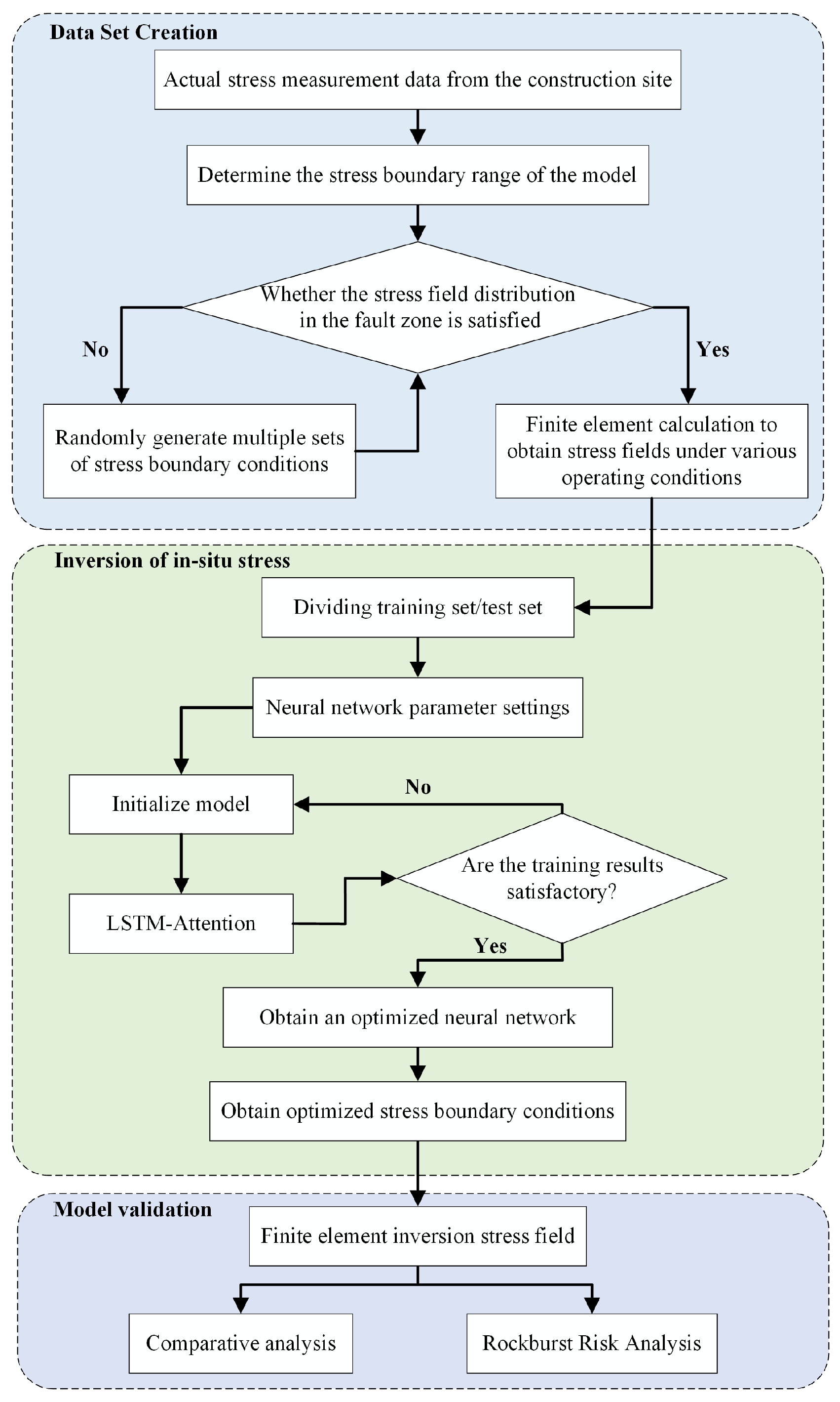
Figure 1. Flowchart for in situ stress inversion technology.
Applsci 15 09567 g001
Figure 3. Three-dimensional geological model.
Applsci 15 09567 g003aApplsci 15 09567 g003b
Figure 4. Comparison of ZK60 measured values and inverted values.
Applsci 15 09567 g004
Figure 5. Comparison of ZK59 measured values and inverted values.
Applsci 15 09567 g005
Figure 6. Comparison of ZK65 measured values and inverted values.
Applsci 15 09567 g006
Figure 7. The distribution of principal stress at depth of 100 m in borehole ZK65.
Applsci 15 09567 g007aApplsci 15 09567 g007b
Figure 8. The distribution of principal stress at depth of 200 m in borehole ZK65.
Applsci 15 09567 g008aApplsci 15 09567 g008b
Figure 9. The distribution of principal stress at depth of 300 m in borehole ZK65.
Applsci 15 09567 g009aApplsci 15 09567 g009b
Figure 10. The features of the minimum principal stress on the regional vertical profile.
Applsci 15 09567 g010aApplsci 15 09567 g010b
Figure 11. The direction of the principal stress on the regional vertical profile.
Applsci 15 09567 g011
Table 1. The occurrence of main faults of the hydropower station.
Serial Number of Fault GroupsOccurrenceIncluded Angle with the Chamber Axis
1110~25° NW∠35~66°Large
2310~330° SW∠35~48°Large
3335~340° SW∠55~70°Large
415~30° NW∠55~60°22~57°
5325~350° SW∠55~70°52~77°
6320° SW (NE)∠75°82°
Table 2. Mechanical parameters of rock masses.
LithologyElastic Modulus
/GPa
Poisson’s RatioDensity
/(kg/m3)
Biotite quartz schist41.330.232730
Chlorite schist48.290.222800
Sandstone64.080.222650
Table 3. Mechanical parameters of faults.
Fault
Parameters
Normal Stiffness
/GPa
Shear Stiffness
/GPa
Cohesion
/MPa
Internal Friction Angle
20150.2215
Table 4. Results of in situ stress of boreholes ZK59, ZK60, and ZK65.
BoreholeSerial NumberDepth
/m
Stress Value
/MPa
Direction of SH
SHShSv
ZK59136.00–36.8012.117.256.04N3° W
256.00–56.809.955.256.57
362.00–62.809.815.316.72N10° E
470.00–70.8010.696.696.93
579.30–80.1014.287.787.18
ZK60124.00–24.802.472.246.91
243.00–43.803.342.427.41
356.00–56.808.254.757.75
466.00–66.809.155.158.02N8° E
576.30–77.1010.356.958.29
ZK651112.40–113.204.903.102.94N17° W
2184.30–185.105.913.014.82
3193.20–194.0013.197.795.06
4239.40–240.2013.397.856.26
5269.30–270.1013.887.847.05
6290.30–291.1012.096.447.60
7299.80–300.6010.785.647.84
8335.50–336.3013.486.998.96
9348.10–348.9011.825.919.11
10353.10–353.9013.627.069.24
Notes: Sh is minimum horizontal principal stress; SH is maximum horizontal principal stress; Sv is vertical principal stress. The vertical principal stress Sv is calculated based on the overburden rock density of 2670 kg/m3. The fracturing section length is 0.80 m.
Table 5. Compressive stress boundary conditions.
NumberBoundary DirectionGravitational Acceleration
m/s2
x/MPay/MPa
1888
28810
38812
410108
510109.8
6101010
7101012
812128
9121210
10121212
Table 6. Statistics of inversion and measured values of geostress components.
BoreholeSerial NumberResultsStress Components
/MPa
σxxσyyσzz
ZK601Measured value2.141.242.24
Inversion value3.271.862.42
Absolute error0.570.310.09
2Measured value2.891.672.42
Inversion value4.172.742.27
Absolute error0.640.540.08
3Measured value7.144.134.75
Inversion value6.543.784.27
Absolute error0.300.170.24
4Measured value7.924.585.15
Inversion value5.993.855.02
Absolute error0.970.360.07
5Measured value8.965.186.95
Inversion value6.634.016.13
Absolute error1.160.590.41
ZK591Measured value10.496.067.25
Inversion value10.146.877.58
Absolute error0.180.400.16
2Measured value8.624.985.25
Inversion value7.594.205.14
Absolute error0.520.390.05
3Measured value8.504.915.31
Inversion value8.775.966.10
Absolute error0.130.520.40
4Measured value9.265.356.69
Inversion value10.035.036.62
Absolute error0.380.160.03
5Measured value12.377.147.78
Inversion value12.627.217.61
Absolute error0.130.040.09
ZK651Measured value4.242.452.94
Inversion value4.252.463.25
Absolute error0.010.000.16
2Measured value5.122.964.82
Inversion value5.132.975.50
Absolute error0.000.000.34
3Measured value11.426.605.06
Inversion value7.234.185.58
Absolute error2.101.210.26
4Measured value11.606.706.26
Inversion value11.606.656.65
Absolute error0.000.020.20
5Measured value12.026.947.05
Inversion value11.746.736.92
Absolute error0.140.100.07
6Measured value10.476.057.60
Inversion value11.226.447.10
Absolute error0.380.190.25
7Measured value9.345.397.84
Inversion value10.856.227.18
Absolute error0.750.410.33
8Measured value11.676.748.96
Inversion value11.626.677.55
Absolute error0.020.040.70
9Measured value10.245.919.11
Inversion value10.245.899.76
Absolute error0.000.010.33
10Measured value11.806.819.24
Inversion value10.766.199.81
Absolute error0.520.310.28
Table 7. Evaluation index values for different principal stresses in ZK65 boreholes.
Principal StressEvaluation of Indicators
RMSEMAEMAPE (%)R2
Maximum principal stress1.46840.78408.35480.8804
Intermediate principal stress0.84460.46308.57100.8824
Minimum principal stress0.66480.58208.35680.9190
Table 8. Model robustness analysis results.
OutliersEvaluation of Indicators
RMSEMAEMAPE (%)R2
0%0.66480.58208.35680.9190
1%0.74620.69439.12400.9014
2%0.95320.867410.37840.8939
3%1.86400.984211.76490.8694
Table 9. Calculation results of other models.
ModelEvaluation of Indicators
RMSEMAEMAPE (%)R2
SVR2.20371.176012.53220.3251
MLR1.26610.692012.82190.3314
GA-BP0.59320.44006.27470.6620
LSTM–Attention0.66480.58208.35680.9190
Table 10. Cavern stress parameters of the chamber.
Depth
/m
SH
/MPa
Sh
/MPa
Sv
/MPa
Angle/°σmax
/MPa
σθmax
/MPa
Rc
/MPa
σ θ R c R c σ max
274.3 m14.287.787.183910.423.9730.337.05
Note: σθmax is the maximum tangential stress.
Table 11. Engineering mitigation measures corresponding to different rockburst risks.
Rock Burst LevelRecommended Engineering Mitigation Measures
No rockburstsNone
Weak rockburstsShort excavation lengths reduce disturbance to the surrounding rock; stress-relief holes should be made when necessary.
Medium rockburstsThe system is equipped with high-prestressed anchor bolts, and flexible protective nets are added in key areas to prevent rock fragments from being ejected.
Strong rockburstsBefore excavation, advance anchor bolts are installed, or pre-decompression blasting is carried out to form a stress buffer zone.
Disclaimer/Publisher’s Note: The statements, opinions and data contained in all publications are solely those of the individual author(s) and contributor(s) and not of MDPI and/or the editor(s). MDPI and/or the editor(s) disclaim responsibility for any injury to people or property resulting from any ideas, methods, instructions or products referred to in the content.