Design and Characterization of Negative-Stiffness Lattice Structures for Diabetic Midsoles

Featured Application

Negative-stiffness lattice structures represent a groundbreaking class of mechanical metamaterials capable of redistributing pressure in highly efficient and adaptive ways. Thanks to their unique ability to undergo localized deformation while maintaining global structural integrity, these lattices are ideal for applications requiring uniform load distribution, energy absorption, and enhanced comfort. From biomedical implants to aerospace panels and protective equipment, their tunable mechanical response opens new frontiers in design and performance.

Abstract

Diabetes mellitus often leads to peripheral neuropathy that compromises protective sensation in the feet and raises ulcer risk through mechanical overload. While prior research has introduced cellular-metamaterial-based shoe midsoles for dynamic plantar pressure redistribution, this study advances the field by delivering a complete, application-oriented workflow for physical prototyping and mechanical validation of such structures. Our pipeline integrates analytical synthesis of curved-beam unit cells, process calibration, and fabrication via thermoplastic polyurethane (TPU) fused-filament fabrication, producing customized, test-ready lattices suitable for future gait-simulation studies and in vivo assessment. Printed TPU tests showed a Young’s modulus of 44.5 MPa, ultimate tensile strength of 4.9 MPa, and strain at break ≈ 20% (Shore 84.5 A/37.2 D). The cellular unit’s compressive response was quantified by theoretical force-threshold estimates and controlled compression tests, enabling data-driven selection of unit cell geometry and arrangement for effective offloading. The response is rate-dependent: higher loading speed increases peak force and hysteresis, indicating that loading rate should be treated as a design parameter to tune dynamic behavior for the target application. Although the analytical model overestimates forces by roughly 50% on average relative to experiments, it accurately captures the influence of key geometric parameters on peak force. Accordingly, experimental data can identify cell strategic geometric parameters (i.e., Q), while the achievable maximum force can be predicted from the model by applying an appropriate correction factor. By connecting modeling, calibration, and experimental validation in one coherent path, the proposed workflow enables manufacturable lattices with controllable activation thresholds for plantar pressure redistribution and provides a practical bridge from concept to application.

1. Introduction

Diabetes mellitus is a chronic condition characterized by insufficient insulin production or resistance leading to hyperglycemia, causing severe organ damage [1]. Without proper control, diabetes can lead to complications such as peripheral neuropathy and causing tingling, pain, and reduced sensitivity in the lower limbs, a major symptom of diabetic foot. Diabetic foot involves changes in the lower limbs, leading to ulcers and potential amputation caused by increased plantar pressure due to excessive mechanical load [2,3]. Thus, the prevention focuses on reducing plantar pressures by prescribing custom-made footwear or orthotics to accommodate foot deformities by redistributing loads [4,5].

Patient-customized cushioned insoles of different materials can redistribute plantar pressures; however, this static unloading mechanism does not prove effective because the sites of high pressure tend to change over time, thus implying frequent changes with consequent costs and timing. The static pressure relief mechanism also does not provide adequate control of pressures, as the areas most subject to repetitive stress are unloaded by transferring the load to other plantar zones, which in turn become at risk of ulceration. Within this scenario, the availability of dynamic-unloading-mechanism-based insoles that can adapt to changes in plantar pressures is a challenge to be pursued.

The aim of this paper is to propose a methodological approach for the design and characterization of novel cellular metamaterials, based on compliant mechanisms, for the fabrication of diabetic foot orthoses capable of redistributing plantar pressures. The paper presents, from both a methodological and experimental perspective, the tuning of the FFF process and the mechanical characterization of the bulk material. The mechanical behavior of the unit cell is also investigated through an analytical model and compared with experimental results. Finally, the complete midsole design approach is developed, while the manufacturing of the full shoe incorporating the designed midsole, along with its characterization, is planned as part of future work.

2. Background

Recent insole research has explored several solutions with optimization frameworks to reduce peak plantar pressures, supported by dynamic numerical models validated experimentally [6,7]. Through the rational design of size, shape, and topology, components based on specific materials can achieve distinct and exotic mechanical properties. Such structures, when subjected to external stresses, undergo structural changes that determine their mechanical response, and deviations from normal elastic behavior are embedded in the deformation modes encoded within their geometry [8,9]. Among these structures, those capable of absorbing energy [9] play an important role; an adequate design allows energy to be stored during deformation by exploiting the bending of specific constituent segments. These yielding mechanisms achieve movement without the use of kinematic torques, relying on the deformation of their parts. In several cases, the design of yielding mechanisms is based on elastic elements exhibiting ‘snap-through’ buckling behavior [10,11] that refers to a buckling type allowing the structure to pass abruptly from one configuration to another under external loads beyond critical values. Multistability refers to a structure’s ability to reach and maintain stable positions different from its original position due to deformation energy accumulation during movement [12]. In the case of certain cellular metamaterials, such as hexagonal honeycomb cells, considerable energy is absorbed, often due to plastic deformation, making the absorbed energy unrecoverable and preventing reuse of the structure. To make the structures reusable (i.e., passive shape reversibility), several studies have focused on designing monostable structures that exploit similar buckling concepts but remain in the elastic field, allowing them to return to their original shape once the load is removed [13,14]. The recent literature presents innovative honeycomb cells with negative stiffness that provide high levels of initial stiffness, compressive strength, and energy absorption, in a reversible manner [15,16]. Reversibility in the deformation of metamaterial structures is often achieved by exploiting the mono/bistability of straight inclined beams or sine-shaped beams. This strategy is widely adopted as the deformation of such structures is elastic, allowing for recoverable energy absorption and a return to the original shape in the absence of loads [17,18]. The curved-beam bistable mechanism exploits the bistability of transversely loaded sinusoidal beams; due to the yielding of the curved beams, the structure exhibits negative-stiffness behavior, programmable based on the geometric parameters of the beam [16]. Unlike elastic elements with a positive slope of the force–displacement curve, elements with negative stiffness show a reduction in force values as displacement increases, creating a region of negative stiffness. This behavior can be exploited to achieve recoverable energy absorption in elastic systems, preventing forces above a given threshold from being transmitted to an isolated mass. Within this paper, we aim to combine the concepts of cellular materials and the possible reversibility of compliant structures through the design of a novel workflow for physical prototyping and mechanical validation of such metamaterials with specific deformation and energy absorption capabilities. To address this, one strategy is to incorporate curved beams with negative stiffness in configurations similar to traditional honeycombs, thus combining high initial stiffness and reversible energy absorption, achieved by programming each cell to deform itself for specific force thresholds. In this context, the proposed geometric model has been validated and tested on the basic cellular structure and on its three-dimensional repetitions, laying the foundation for the development of smart customized midsoles capable of automatically redistributing the load when a localized pressure threshold is exceeded.

While prior research has introduced cellular metamaterials for dynamic plantar pressure redistribution, this study advances the field by developing a complete, application-oriented workflow for physical prototyping and mechanical validation of such structures. Together, these elements bridge conceptual design and practical implementation, delivering test-ready, clinically targeted lattices with controllable activation thresholds.

3. Materials and Methods

A methodological approach to the design and development of architected materials is proposed to embed the lattice structure with the intended mechanical and functional requirements. The proposed workflow, summarized in Figure 1, integrates geometric parametric design, material characterization, and functional modeling to guide the development of smart lattice-based midsoles from a unit cell model. The approach addresses key requirements such as the implementation of a reversible offload mechanism (i.e., negative-stiffness behavior) and its printability through Fused Filament Fabrication (FFF) Additive Manufacturing (AM) processes.

3.1. Geometric Modeling

Negative stiffness can be achieved by managing the shape of the structure elements and their geometric relationships, which can be selected from various options available in the literature [13,19,20]. For the purpose of this study, a cellular structure based on a honeycomb with sinusoidal curved elements was selected [15,21]. Depending on element dimensions, this cellular structure can exhibit different mechanical behavior (i.e., stable or bistable behavior). Figure 2 shows the unit cell. The highlighted parameters define the overall dimensions of the structure and refer to the parameters listed in

Table 1. Meaning of the parameters in Figure 2.

t	Curved beam thickness	h	Amplitude of the cosine curve
H	Unit cell height	d	Distance between the curved beams
t2	Thickness of horizontal beams	s	Thickness of vertical supports
L	Cell size/cosine wavelength	b	Depth of the cell

. The geometric parameters were selected based on the application, considering the results of analytical, numerical, or experimental models, as described below. The minimum height H/2 considers the deformation of the beams in such a way that, once fully deformed, they do not come into contact with the horizontal supports, thus altering the behavior and compression response of the cells.

3.2. Material

In general, the material can be selected by adopting methodological approaches that provide an optimal solution for a specific design context [22]. In this work, thermoplastic polyurethane (TPU) material was selected for its properties between the characteristics of plastic and rubber, such as elasticity, abrasion resistance, and weather resistance, including exposure to UV light and moisture [23], which make it suitable for applications such as components and midsoles [24,25,26]. TPU combines the mechanical performance of rubber with the processability of thermoplastics, effectively bridging the gap between rubber and plastics [27,28]. This enables TPU to be widely employed in Fused Filament Fabrication (FFF) [29]. To integrate the information provided by the manufacturers, FFF parameter tuning and mechanical characterization tests were carried out, ensuring that the entire AM process was appropriate for the fabrication of the proposed structures.

3.2.1. Process Tuning

In the context of FFF, tuning refers to the process of optimizing various parameters, such as temperature, print speed, retraction, and flow rate, to achieve the best possible print quality and performance [30]. Because of its elastic properties and its FFF printability, the use of TPU material has been widely characterized in the literature [30,31,32]. Nevertheless, every specific TPU material needs fine-tuning to outperform in a specific 3D printer. Temperature and printing speed play a fundamental role in the delamination and integrity of the parts. To ensure proper adhesion between layers, it is advisable to increase the temperature; optimal results have been obtained with a temperature of 5 °C higher than the recommended value [32]. Although not all TPU filaments have the same ideal printing temperature, in several cases, the best results were obtained with a nozzle temperature of 230 °C [28]. In the specific case of TPU, optimal results were achieved by maintaining a slow and constant printing speed. Given the nature of the material, it is suggested to keep a speed around 15–20 mm/s [28], but even at 30 mm/s, good quality was obtained while reducing printing times [32]. To address the problem of stringing (i.e., “strings” of filament between parts of a print, caused by excess material oozing from the nozzle during travel moves), it is recommended to reduce the retraction speed while increasing the retraction distance to prevent unwanted material oozing. In general, reducing the retraction speed proportionally improves the final quality; to achieve these results, a speed of 25 mm/s has been found optimal [31]. Adhesion to the print bed, particularly of the first layers, is a crucial step. To obtain better prints, setting the print bed to a moderate temperature between 40 and 60 °C is sufficient [28,31,32]. Based on the above considerations, the parameters listed in

Table 2. Print parameters set to produce the test cube in Figure 3.

Layer Height	0.1 mm
Line Width	0.4
Wall Line Count	2
Top Layers	0
Bottom Layers	1
Infill	0%
Print Speed	30 mm/s
Printing Temperature	230 °C
Build Plate Temperature	50 °C
Retraction Speed	25 mm/s
Retraction Distance	1 mm

were selected for the FFF process.

Another parameter to consider for improving print quality, especially for thermoplastic elastomeric materials, is the extrusion flow parameter, also known as extrusion rate. The tuning of this parameter is essential to avoid under-extrusion, which results in defective products characterized by undesired low modulus, reduced toughness, and poor surface finish. Conversely, over-extrusion leads to the accumulation of excess material, causing geometrical inaccuracies [33]. This parameter is expressed as a percentage and defines the amount of extruded material, with a nominal value of 100%. An increase in the flow parameter corresponds to a greater volume of filament being extruded through the nozzle, whereas a decrease results in a reduced filament volume. Optimizing this parameter allows for improved surface finish, optimal interlayer adhesion, and enhanced mechanical strength [33]. To identify the optimal flow value, a systematic procedure was implemented [34,35]. As a first step, five measurements of the filament diameter on the filament cross-section, approximately 10 cm apart from each other, were collected by using a caliper. From the obtained values, the average diameter was calculated, and the actual filament diameter was then set in the slicing software. Then, a test cube (Figure 3) consisting of 2 walls and 0% infill was manufactured without top and bottom layers. The values for layer height, temperature, and printing speed were selected based on references from the literature, as previously reported (Table 2). By comparing the nominal and actual wall thicknesses, the flow parameter can be calculated using the following equation: $Flow Rate =100·Nominal\_Wall\_Thickness/Measured\_Wall\_Thickness$, where Measured_Wall_Thickness is the mean value obtained from four thickness measurements taken on each side of the hollow cube. This approach or similar approaches [36] are technically reliable and widely adopted within the 3D printing community. Although these methods are not extensively documented in the scientific literature, they are frequently employed in research contexts—particularly for calibrating the extrusion multiplier of foamed polymers [34,37,38]—as they offer a simplified alternative to complex measurement techniques and modeling. Alternatively, the flow rate can be set to the lowest value at which continuous line connection is achieved during printing [39]. In this work, Sovol SV04 FFF technology was employed for the fabrication of the samples.

3.2.2. Mechanical Characterization

Hardness Test

The ISO 868:2003 standard [40] provides guidelines for determining the indentation hardness properties of plastic materials. According to this standard, two types of durometers, type A and type D, are employed to measure Shore A and Shore D hardness, respectively. Each durometer consists of a pressure foot, approximately 3 mm in diameter, at the center of which is located the indenter, a hardened steel rod with a diameter of about 1.25 mm. The adopted specimen is depicted in Figure 4a. The testing procedure involves placing the specimen on a hard, horizontal surface, holding the durometer vertically, and applying the pressure foot onto the specimen as quickly as possible while keeping it parallel to the surface. Once a stable contact between the foot and the specimen is achieved, the measurement is taken within 1 s. Five measurements at different positions allow for calculating the average hardness value.

Tensile Test

To determine key mechanical properties such as the material’s elastic modulus, tensile tests were performed. Along with hardness measurements, tensile testing is one of the most common mechanical tests used to characterize material behavior. The ISO 527-2:2012 [41] and ISO 527-1:2019 [42] standards specify the general principles for determining the tensile properties of plastic materials under defined conditions and describe the methods for conducting these tests, as well as the resulting stress–strain curves along with the relevant parameters. The printed specimens, shaped like a “dog bone,” were designed according to the standard dimensions, with a gauge length of L0 = 20 mm (Figure 4b). Three specimens were manufactured by orienting the samples along the y-axis (Figure 4c), using the process parameters listed in Table 2 and a flow rate resulting from the tuning process, i.e., 104%. Due to the anisotropic behavior of additively manufactured parts, the mechanical properties of samples are typically evaluated along different directions. In particular, strength is generally lower in the direction perpendicular to the build plane (i.e., the z-direction), while similar values are typically observed along the x- and y-axes. However, in this study, the cell geometry was extruded, and the applied load acted along a direction lying in the x–y plane, with respect to the machine’s reference system. Consequently, for the purposes of this investigation, the characterization of in-plane samples was considered sufficient.

Tensile tests were executed on an MTS Acumen 3 Electrodynamic Test System equipped with a 3 kN load cell and an MTS 634.31 F extensometer. The speed rate was 1 mm/min, the data acquisition rate was set to 20 Hz, and the gauge length was 20 mm. Stress–strain curves were plotted, and Young’s modulus, ultimate tensile strength (UTS), and strain at break ($\epsilon max$) were calculated.

3.3. Cell Mechanical Property Modeling

An analytical model of the unit cell (or half-cell) can be employed to establish the key parameters required for modeling the cell behavior in accordance with the specific application and its functional requirements (i.e., compliant reversible mechanism, threshold force, and corresponding deformation). Such a modeling approach is also essential for identifying the interdependencies among geometric parameters governing the deformation mechanisms, thereby supporting the design of a focused and effective experimental campaign, which is necessary to validate and/or refine the analytical model. Other models not employed in the present study, such as finite-element models, can be used to analyze the mechanical behavior of the cell.

3.3.1. Analytical Model

The curved-beam mechanism design is inspired by buckled straight-beam mechanisms, where a straight beam is compressed to buckle into stable positions on either side. Modeling these buckling modes is essential for accurately representing the curved-beam mechanism. As highlighted in the literature, the parameter governing the force–displacement behavior is $Q$ = h/t. A possible model for a single beam is

$$F\left(\Delta \right)={\displaystyle \frac{3{\pi }^4{Q}^2}{2}}\Delta \left(\Delta -{\displaystyle \frac{3}{2}}+\sqrt{{\displaystyle \frac{1}{4}}-{\displaystyle \frac{4}{3Q^2}}}\right)\left(\Delta -{\displaystyle \frac{3}{2}}-\sqrt{{\displaystyle \frac{1}{4}}-{\displaystyle \frac{4}{3Q^2}}}\right)={\displaystyle \frac{3{\pi }^4{Q}^2}{2}}\Delta \left[{\left(\Delta -{\displaystyle \frac{3}{2}}\right)}^2-\left({\displaystyle \frac{1}{4}}-{\displaystyle \frac{4}{3Q^2}}\right)\right]$$

(1)

$$\Delta ={\displaystyle \frac{\delta }{h}}$$

(2)

$$F={\displaystyle \frac{L^3}{EIh}}f$$

(3)

$$I={\displaystyle \frac{t^{3}b}{12}}$$

(4)

where $F$ is the normalized force, f is the force, $\Delta$ is the normalized displacement, $\delta$ is the displacement, $E$ is the elastic modulus, and $I$ is the moment of inertia [16] (see Figure 2 and Table 1 for the meaning of the other parameters).

The double-beam arrangement allows the structure to support twice as much force as a single beam and enhances its effectiveness in energy absorption. The force threshold compared to a single beam is increased, and complex buckling modes are prevented, ensuring negative stiffness [20]. Consequently, the double-beam configuration is selected for the present work, and the $F$ formula is updated with a scale factor of 2. Thus, the analytical model of the half-cell can be expressed by the following equation:

$$F\left(\Delta \right)=3{\pi }^4{Q}^2·\Delta \left[{\left(\Delta -{\displaystyle \frac{3}{2}}\right)}^2-\left({\displaystyle \frac{1}{4}}-{\displaystyle \frac{4}{3Q^2}}\right)\right]$$

(5)

Depending on the value of $Q$, Equation (5) exhibits the trend shown in Figure 5. This function can exhibit both a maximum and a minimum, which can be identified by setting the first derivative of Equation (4) equal to zero. This occurs when the normalized displacement is

$${\Delta }_{th}=1\pm \sqrt{{\displaystyle \frac{1}{3}}-{\displaystyle \frac{4}{9Q^2}}}$$

(6)

In this context, the negative value ${\Delta }_{th-}$ corresponds to the maximum normalized force $F_{max}=F\left({\Delta }_{th-}\right)$, while the positive value ${\Delta }_{th+}$ indicates the minimum normalized force $F_{min}=F\left({\Delta }_{th+}\right)$, as computed using Equation (5).

By analyzing Equations (5) and (6), for a perfectly elastic material with perfectly rigid boundary conditions, a $Q$ value greater than $4/\sqrt{3}\approx 2.31$ indicates bistability; i.e., the minimum of Equations (1) and (5) is lower than zero. Similarly, for $Q$ less than $2/\sqrt{3}\approx 1.15$, the mechanism does not exhibit negative stiffness. Consequently, for the application considered in the present study, $Q$ should ideally range between 1.15 and 2.31. However, for certain materials, experimental results show that the honeycomb structure does not exhibit bistability up to approximately $Q=2.7$ [43]. Moreover, considering the selected material, i.e., TPU, the constitutive model is nonlinear, and the mechanical behavior is strain-rate-dependent. Phenomena such as softening, hysteresis (with different loading and unloading paths), stress relaxation under constant strain, creep, and residual strain—especially after the first cycle—are observed. Additionally, the mechanical response changes with the number of cycles, tending to stabilize after a few repetitions [27]. Some of these effects, under established conditions, could be accounted for by introducing an empirical correction coefficient in Equation (5), which should be experimentally determined and will be the objective of future works.

3.3.2. Unit Cell Experimental Tests

To establish the physical relation between force and displacement, the unit cell structure was subjected to compression testing using the MTS Acumen^® Electrodynamic Test Systems machine, by MTS Systems, Eden Prairie, MN, USA. The tests were performed while maintaining a speed of 10 mm/min and following a loading–unloading cycle with amplitude 2 h (see Figure 2a). To carry out the tests, the structures were positioned as in Figure 6 on a rigid support plane, centered beneath the loading cylinder. To simulate the constraint conditions of adjacent cells and to prevent lateral deformation of the vertical walls, the structures were positioned within the two vertical rigid supports shown in Figure 6. The application of these constraints is necessary to achieve a mechanical response equivalent to that of multiple consecutive cells.

Based on the preliminary analysis of the analytical model and of the functional requirements, the chosen geometrical parameters for the experimental tests are reported in

Table 3. Geometrical parameters of double-beam structure for experimental tests.

Test ID	$\mathbf{t}$ [mm]	$\mathbf{Q}=\mathbf{h}/\mathbf{t}$
t2.0−Q3.0	2.0	3.0
t2.5−Q2.4	2.5	2.4
t3.0−Q2.0	3.0	2.0

, by considering $h = 6$ mm, $s = 4$ mm, $L = 35$ mm, $H/2 = 35$ mm, $b = 15$ mm, $d=2t$.

3.3.3. Cell Parameter Dimensioning

Based on the described models and considering the functional requirements, it is possible to determine the cell’s geometrical parameters using a trade-off approach. The dimensions for the double-beam cell were set empirically by taking into account several aspects: (i) the intended deformation capability, (ii) the ability to respond to pressures like those expected for diabetic foot application, and (iii) the manufacturability through available technologies (FFF in the present study) [10].

Based on the desired behavior, it is possible to set $Q$ within the range of 1.15 to 2.31, considering that values of $Q$ close to 1.15 lead to a smaller difference between $F_{max}$ and $F_{min}$.

Equation (2) shows that the parameter h has a significant influence on the deformation ${\delta }^{*}$ at which the mechanism transitions to the negative-stiffness regime. As a first approximation, this transition can be assumed to occur when $\Delta =0.5$, or alternatively, it can be calculated using $Q$ through Equation (6). Consequently, once the deformation at which the regime change occurs is established, the value of h can be determined according to

$$h={\displaystyle \frac{{\delta }^{*}}{{\Delta }_{th-}}}$$

(7)

After the h parameter is chosen, t can be calculated according to $Q$:

$$t=h/Q$$

(8)

The critical pressure $p^{*}$, at which load redistribution is necessary to avoid the effects of prolonged high plantar pressure in diabetic patients, is 200 kPa [10]. This pressure can be determined by the ratio between $f_{max}$ and the cell area:

$$p^{*}=f_{max}/Lb$$

(9)

By substituting Equations (3) and (4) into Equation (9), the critical pressure $p^{*}$ can be expressed as a function of the maximum normalized force $F_{max}$ and the relevant geometric and mechanical parameters:

$$p^{*}= F_{max}{\displaystyle \frac{EIh}{L^3}}{\displaystyle \frac{1}{Lb}}= F_{max}E{\displaystyle \frac{t^{3}h}{12L^4}}$$

(10)

By observing Equation (10), it can be seen that the parameter $b$ has no influence on the critical pressure $p^{*}$. Furthermore, the maximum normalized force $F_{max}$ depends solely on $Q$. The elastic modulus $E$ is an intrinsic material property, whereas $h$ and $t$ have been previously defined. Consequently, the only parameter to be determined is L.

The other parameters have no significant influence on the results and can be selected based on manufacturing constraints or to minimize the overall cell dimensions. These results should be corrected by a coefficient derived from experimental data.

3.4. Midsole Development

Figure 7 illustrates the procedure for modeling the midsole, taking into consideration the manufacturing steps. Based on the above considerations and experimental results, a unit cell is modeled using the geometrical parameters reported in

Table 4. Geometrical parameters of the unit cell.

Q	h [mm]	t [mm]	t2 [mm]	D [mm]	L [mm]	H/2 [mm]	s [mm]	b [mm]
2.31	3	1.3	2	2.6	17.5	18	2.6	15

.

To decouple the stress between adjacent elements, the whole midsole can be modeled as a set of stripes of cells (Figure 7a). Techniques based on free-form deformation (FFD) adopting non-uniform rational basis splines (NURBSs) allow conforming a regular lattice structure to the real sole shape [44]. Figure 7b shows the shape of the bottom surface of the insole, extended to its bounding box to avoid excessive deformation of the stripes during the FFD process and simplify the 3D printing process. The result of the FFD is shown in Figure 7c. The deformed stripes are then limited to the volume between the outer sole and the insole (Figure 7d). The stripes are rotated to avoid overhang and supports during the 3D printing process (Figure 7e). Before being inserted into the outer sole, the stripes are joined by some further curved layers. This is achieved by developing a specific fixture (Figure 7f) that is used for positioning the single stripes (Figure 7g) in the FFF 3D printer. At the end of the printing of the fixture, the process is paused, the stripes are positioned, and the process restarts following a specifically developed toolpath (Figure 7h). Figure 8 shows the proposed manufacturing process on flat stripes, which takes inspiration from a previous work [45]. Finally, the midsole can be inserted into the outer sole as shown in Figure 7i.

Due to the deformations that occur during the geometric modeling process performed to adapt the cell to a curved surface, the actual dimensions of the cell elements may slightly differ from those of the initial design. In addition to the objectives of the present study, it is therefore necessary to manufacture and test the proposed system under real-life conditions, such as during walking, to verify the actual behavior of the midsole. This can be achieved by integrating one of the systems available in the literature for measuring foot plantar pressure [46].

4. Experimental Results

To evaluate the mechanical response of the proposed structures, the results of the experimental test and analytical model are reported and compared in this section.

4.1. Material Characterization

4.1.1. Manufacturing Process Tuning

As part of the tuning procedure, five measurements of the filament diameter were taken (

Table 5. Measured filament diameter values.

Measured Filament	Diameter Values
1	1.77 mm
2	1.78 mm
3	1.77 mm
4	1.76 mm
5	1.77 mm
Average value	1.77 mm

). The average value was subsequently computed and set as the actual filament diameter in the slicing software.

To calculate the optimized flow rate, the model shown of Figure 3 was manufactured using the process parameters listed in Table 2.

Table 6. Results of the wall thickness measurements on the four sides of the test cube.

Test Cube Side	Wall Thickness
1	0.76 mm
2	0.77 mm
3	0.77 mm
4	0.78 mm
Average value	0.77 mm

reports the measured wall thickness, which is compared to the nominal value (0.8 mm), resulting in a flow rate calculated as

$$Flow Rate={\displaystyle \frac{Nominal\_Wall\_Thickness }{Measured\_Wall\_Thickness}}={\displaystyle \frac{0.8}{0.77}} \approx 1.0389$$

(11)

This value, approximated to 104%, was then used in the slicing settings for all subsequent tests.

4.1.2. Mechanical Characterization Results

To evaluate the mechanical response of the printed TPU material, hardness tests were conducted on cylindrical specimens. As shown in Figure 9, the tested sample consists of a vertically printed cylinder, for which measurements were taken on the bottom layer and the top layer.

The results of the measurements are reported in

Table 7. Hardness test results.

		Shore A		Shore D
Top layer	1	85.5	1	38
	2	85.5	2	37
	3	86.5	3	39
	4	88	4	40
	5	87.5	5	38.5
	Mean	86.6	Mean	38.5
	SD	1.14	SD	1.12
Bottom layer	1	81.5	1	35.5
	2	81	2	35
	3	83.5	3	35.5
	4	84.5	4	37
	5	82	5	36
	Mean	82.5	Mean	35.8
	SD	1.46	SD	0.68

. According to hardness measurement standards, a Type A durometer is recommended when Shore D values are below 20, whereas a Type D durometer is more suitable for harder materials, when Shore A values exceed 90. Given the intermediate range of the measured values, both Shore A and Shore D hardness scales were applied to provide a complete characterization. Notably, the printing process appears to influence hardness slightly: the first printed layer (bottom layer) was on average 5.8% softer than the last printed layer (top layer). This difference is likely due to variations in surface conformation and thermal history during the printing process. The average Shore hardness values obtained for the TPU specimen were 84.5 HA (Shore A) and 37.2 HD (Shore D). These values confirm the material’s elastomeric behavior, suitable for cushioning and energy absorption applications.

Figure 10 illustrates the stress–strain behavior of the dog-bone specimens shown in Figure 4b, which were subjected to tensile testing.

The elastic modulus of the material was calculated as the slope of the fitting straight line in the strain range between 1 and 5%. By analyzing the curves, it is possible to derive the mean values of the Young’s modulus (E), ultimate tensile strength, and elongation at break, which are 44.5 MPa, 4.9 MPa, and 20%, respectively.

4.2. Cell Mechanical Properties

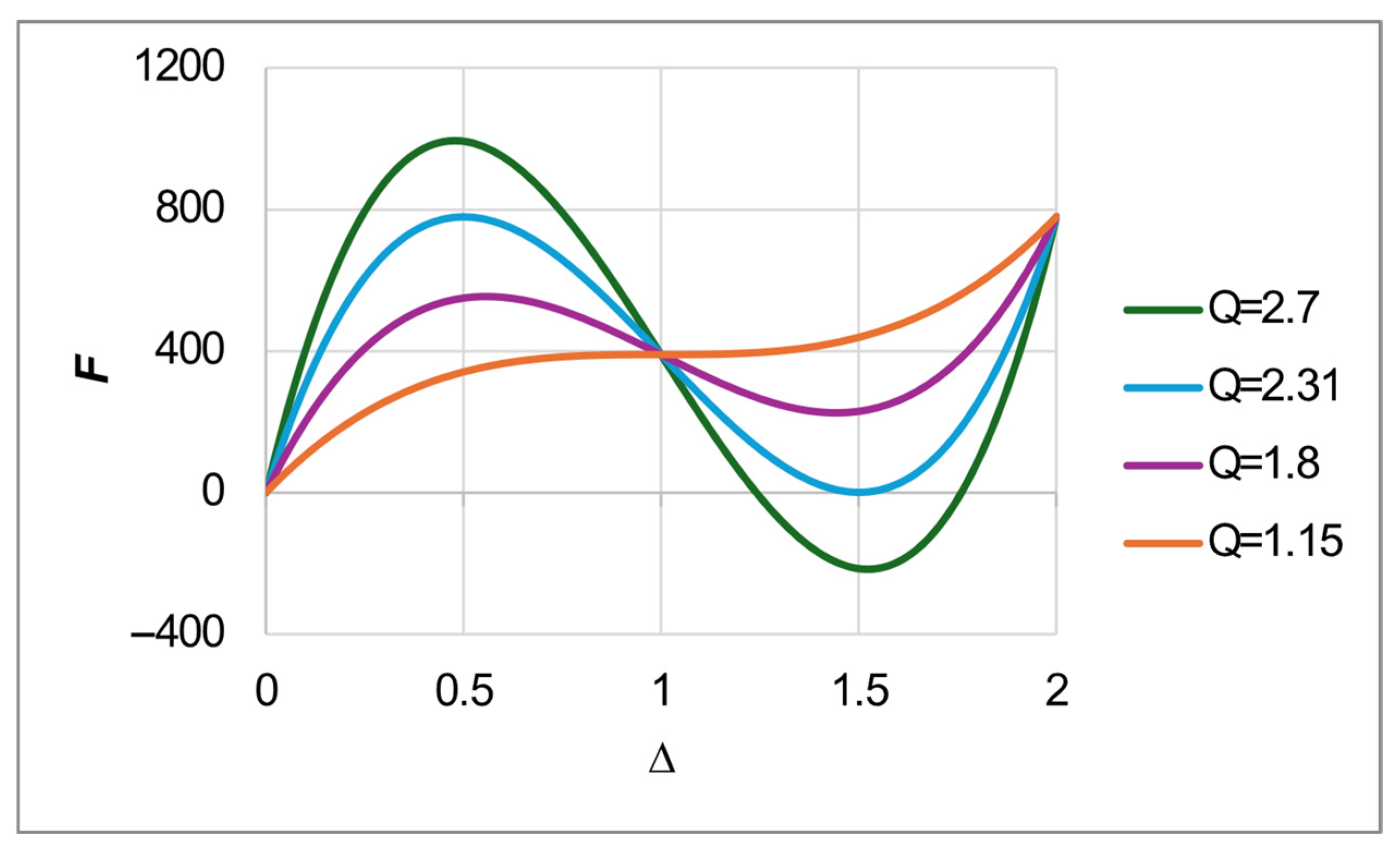
Figure 11 illustrates the behavior of the analytical model in terms of force and displacement, obtained by combining Equations (2), (3), and (5) for the case studies considered, while

Table 8. Main characteristics of the tested cells based on analytical model.

Test ID	${\Delta }_{\mathit{t}\mathit{h}-}$	${\mathit{F}}_{\mathit{m}\mathit{a}\mathit{x}}$	${\mathit{\delta }}_{\mathit{m}\mathit{a}\mathit{x}}$[mm]	${\mathit{f}}_{\mathit{m}\mathit{a}\mathit{x}}$[N]	${\Delta }_{\mathit{t}\mathit{h}+}$	${\mathit{F}}_{\mathit{m}\mathit{i}\mathit{n}}$	${\mathit{\delta }}_{\mathit{m}\mathit{i}\mathit{n}}$[mm]	${\mathit{f}}_{\mathit{m}\mathit{i}\mathit{n}}$[N]	${\mathit{f}}_{\mathit{ratio}}$
t2.0−Q3.0	0.467	1185.5	2.8	73.8	1.53	−406.3	9.2	−25.3	1.34
t2.5−Q2.4	0.494	826.1	2.96	100.5	1.51	−46.9	9.04	−5.7	1.06
t3.0−Q2.0	0.529	634.5	3.17	133.4	1.47	144.7	8.83	30.42	0.77

summarizes the main characteristics of the tested cells based on the analytical model. In this context, the force ratio, $f_{ratio}$, is also introduced, representing the ratio between the force decay and the maximum force, i.e., $(f_{max}- f_{min})/f_{max}$. It can be observed that increasing $t$ leads to an increase in both $f_{max}$ and $f_{min}$, while $f_{ratio}$ decreases. An analysis of the relevant equations reveals that an increase in $h$ results in an increase in $f_{max}$ and $f_{ratio}$ and a decrease in $f_{min}$. Notably, $h$ is the only parameter that affects displacement, as greater values of $h$ lead to larger deformations (see Equation (2)). As previously discussed, the bistability condition depends simultaneously on both $t$ and $h$, through the parameter $Q$. Among the cases presented, only the configuration t2.0−Q3.0 does not result in bistability. Moreover, increasing $b$ and $E$, results in an increase in $f_{max}$ and $f_{min}$, while $f_{ratio}$ remains the same. Finally, increasing $L$ results in a decrease in $f_{max}$ and $f_{min}$, while $f_{ratio}$ remains unchanged.

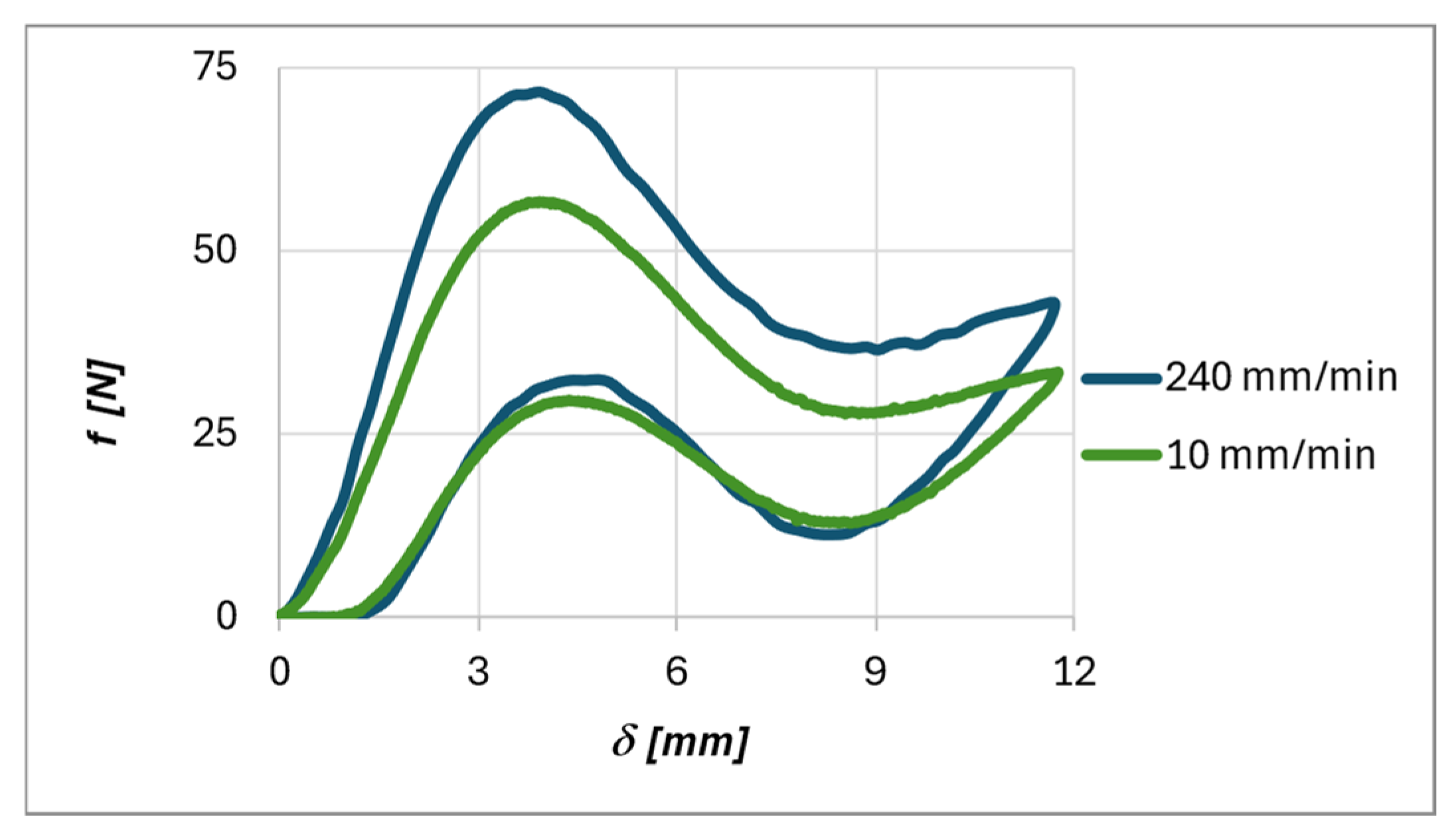
Figure 12 represents the force–displacement data obtained during the compression tests on the manufactured samples, while Figure 13 shows the behavior of sample t2.5−Q2.4 at different loading rates.

Table 9. Main features of the experimentally tested cells. Parameters marked with a prime (′) refer to the loading phase, whereas those marked with a double prime (″) correspond to the unloading phase.

Test ID	${\mathit{\delta }\mathit{\prime }}_{\mathit{max}}$[mm]	${\mathit{f}\prime }_{\mathit{max}}$[N]	${\mathit{\delta }\prime }_{\mathit{min}}$[mm]	${\mathit{f}\prime }_{\mathit{min}}$[N]	${\mathit{\delta }″}_{\mathit{max}}$[mm]	${\mathit{f}″}_{\mathit{max}}$[N]	${{\mathit{\delta }}^{″}}_{\mathit{min}}$[mm]	${\mathit{f}″}_{\mathit{min}}$[N]	${\mathit{f}}_{\mathit{ratio}}$
t2.0−Q3.0	2.67	35.62	7.91	10.68	2.09	12.81	7.40	3.80	0.70
t2.5−Q2.4	3.91	57.00	8.53	27.82	4.37	29.74	8.62	12.81	0.51
t3.0−Q2.0	3.63	70.25	9.57	40.97	4.47	38.37	8.10	25.04	0.42

summarizes the most significant values from the tests presented in Figure 12 and Figure 13. As expected, during the loading phase, the curves show an initial segment with positive stiffness, followed by a region with negative stiffness, and then again, a segment with positive stiffness. A similar behavior is observed during the unloading phase, although the force values are lower for the same displacement, and a residual displacement is present when the force returns to zero. It is possible to observe that both the maximum force (${f\prime }_{max}$) and the minimum force (${f\prime }_{min}$) during loading are higher than those during unloading (${f″}_{max}$ and ${f″}_{min}$). The ratio between the maximum forces during loading and unloading increases with t, with an average value of 52%. A similar trend is observed for the minimum forces. These differences are associated with the energy dissipated during the loading–unloading cycle, which is represented by the area enclosed in the loop shown in Figure 12 and Figure 13. This phenomenon is known as hysteresis. Figure 12 also highlights that higher values of t and Q lead to higher force–displacement curves. In contrast, the differences between the curves at different loading rates are related to the material’s time dependence. As can be seen in Figure 13, higher loading rates lead to higher forces. These phenomena are thoroughly documented in the scientific literature for other types of samples [27].

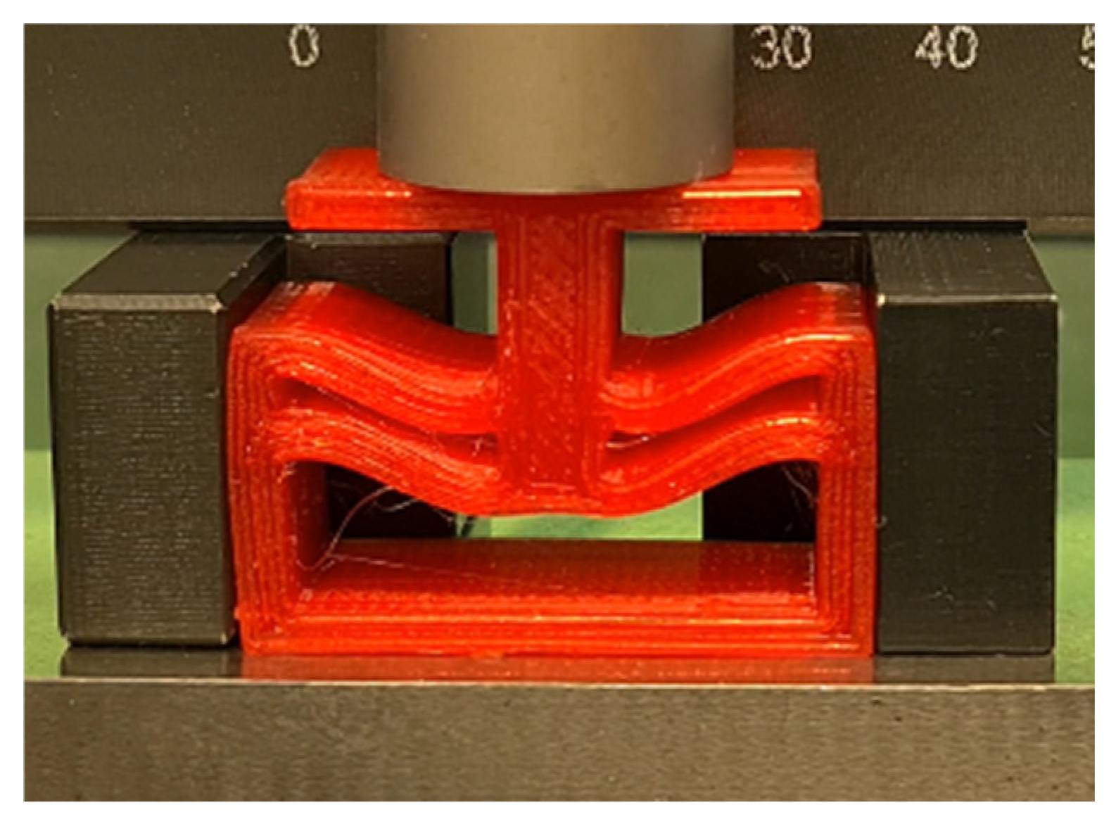
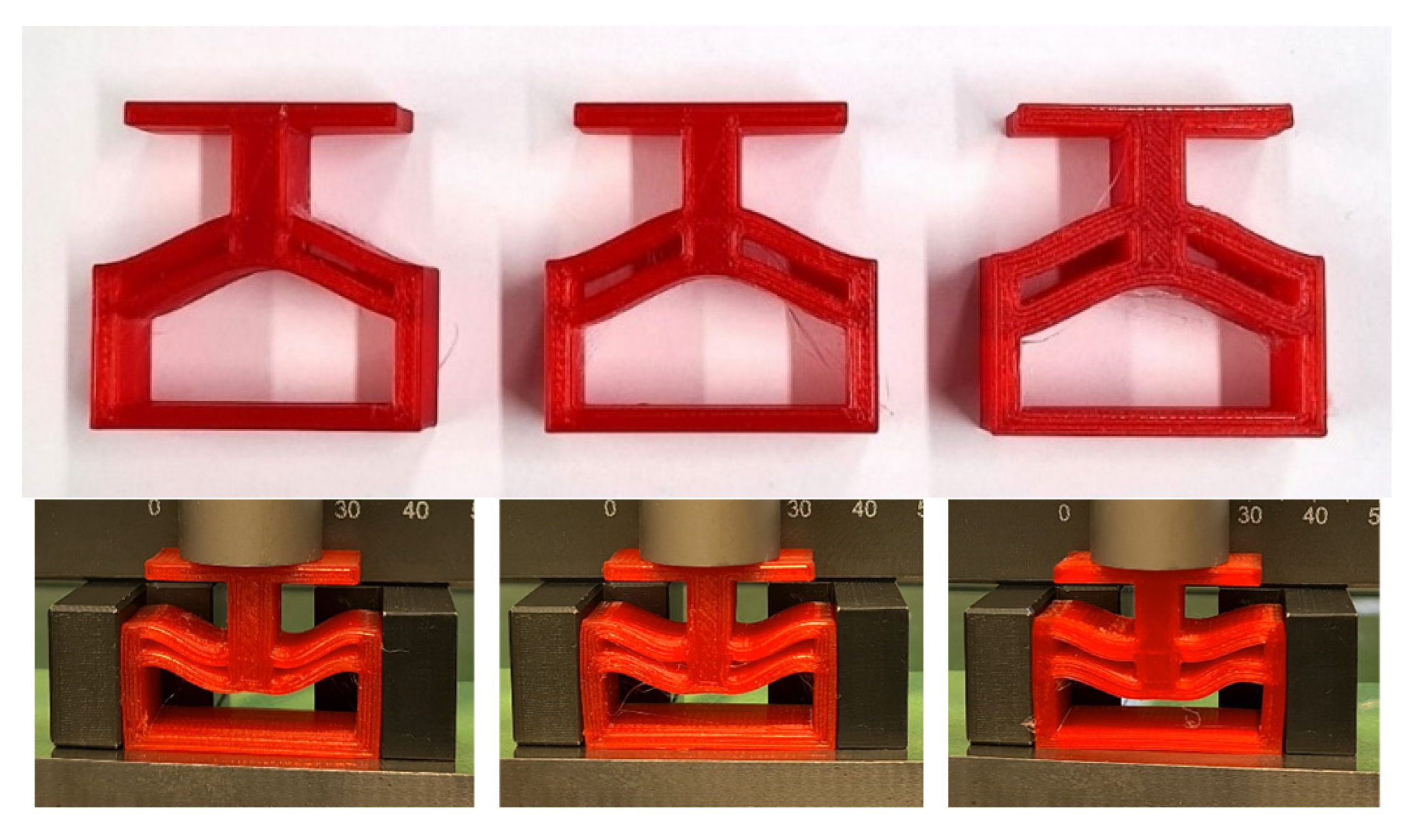
Figure 14 illustrates the fabricated samples along with their deformation mechanism under compressive loading. As observed, unlike the idealized model, the vertical walls undergo lateral deformation despite the presence of vertical rigid guides. This is one of the factors contributing to the discrepancy between the experimental results and the analytical model. In fact, these undesired boundary conditions redistribute the strain energy, leading to lower measured peak forces. Although the experimental behavior aligns with the numerical model, the measured maximum force, ${f\prime }_{max}$, is on average 47% lower than the theoretical prediction.$f_{ratio}$ exhibits a similar behavior, showing an average reduction of approximately 48%, with a corresponding effect on $f_{min}$. The deviation in displacement corresponding to the maximum and minimum force is, on average, 17% and 9%, respectively. This result may be related to the definition of the starting point of the curve, which may exhibit a settling behavior of the specimen in its initial region. Furthermore, bistability is not observed in any of the experimental configurations. For midsole offloading, we seek a monostable, recoverable behavior so that after each walking step, the structure returns to its initial state without the application of negative external forces. Under the chosen material (TPU) and boundary conditions, the tested geometries exhibit a monostable response, ensuring reversible offloading and avoiding snap-through “locking.” Accordingly, the adopted Q values are appropriate for the target application, where a reliable reset to the initial configuration is required.

To strengthen interpretation, link observations to mechanisms, and provide actionable guidance for design and future optimization, it is worth noting that the analytical model assumes linear elasticity, whereas TPU [27,47]

-

Exhibits nonlinear, large-strain elastomeric behavior.

-

Displays a large hysteresis loop with residual strain upon unloading, which is only partially recovered over time.

-

Shows time-dependent behavior; i.e., the material responds differently depending on the strain rate.

-

Manifests Mullins-type softening, i.e., the stress–strain curve in the second cycle is significantly more compliant than that in the first, with stable curves typically observed after only four cycles.

Consistently, Figure 10 exhibits nonlinear behavior, Figure 12 and Figure 13 show a large hysteresis loop with residual strain, and Figure 14 presents time-dependent behavior where higher test speed leads to higher force and increased hysteresis. The study of the softening mechanism will be addressed in future work.

Despite the differences between the analytical model and the experimental data, the analytical model adequately captures the influence of the geometrical parameters on the maximum force. Therefore, the experimental results, potentially integrated with additional data, can be used to correct the model, enabling the design of midsoles that more accurately reflect actual conditions.

4.3. Model Behavior and Sensitivity Analysis for Parameter Selection

As discussed in Section 3.3.3, the geometrical parameters influencing the analytical model are $h, t, L,$ and $E$. An analysis of the behavior of the critical pressure p* based on these parameters allows for a better understanding of the phenomenon.

Figure 15 shows the behavior of $Q$ and $f_{ratio}$, as functions of $h$ and $t$. It can be observed that increasing either $h$ or $t$ leads to an increase in $Q$. Considering the experimental results, which show that the force decay is half the nominal value, it is reasonable to assume a value of $Q$ equal to 2.31. This corresponds to a theoretical $f_{ratio}$ of 1 and an effective value of approximately 0.5.

Figure 16 shows the behavior of δ* and δ_min as functions of h and t. These parameters mainly depend on $h$ (see Equation (2)). The selected value of Q leads to ${\Delta }_{th-}=0.5$ Assuming ${\delta }^{*}=1.5 \mathrm{mm}$, the deformation at which the mechanism transitions to negative stiffness, Equation (7) yields h = 3 mm. Moreover, according to Equation (8), t = 1.3 mm.

Once the material is selected and E is known, in this specific case derived from experiments (E = 44.5 MPa), Equation (10) yields L = 17.5 mm. Figure 17 shows the behavior of p* and p_min, as functions of $h$ and $t$, for L = 17.5 mm and E = 44.5 MPa. This analysis can be useful to confirm whether the selected pair of parameters meets the pressure threshold requirement, or to identify an alternative combination of h and t that satisfies the same condition. Figure 18 presents the analytical model of the cell based on the calculated parameters, along with a hypothetical expected behavior derived from experimental results integrated into the model, which will be the focus of future work.

A sensitivity study was carried out to evaluate the effects on p* of variations in the parameters influencing cell behavior in the vicinity of the selected values. The results are summarized in

Table 10. Effect of parameter variation on p*.

Parameter Variation	p* Variation
	h	t	L	E
−1%	−4.6%	−3.7%	1.8%	−1.0%
1%	4.8%	3.7%	−1.8%	1.0%

. The parameters with the greatest influence on p* are h and t: a 1% variation in h leads to a 5% change in p*, while a 1% variation in t results in a 4% change. p* is proportional to 1/L⁴, as can be observed by analyzing Equation (10). A 1% variation in L leads to a 2% change in p*, while a 1% variation in E results in a 1% change, due to its linear proportionality.

5. Conclusions

This study aimed to investigate and validate the behavior of compliant mechanisms for the design of diabetic foot insoles capable of redistributing plantar pressures and reducing localized mechanical stress. The focus was on curved-beam-based deformation units, exploiting elastic instability under transverse loading. Analytical modeling and experimental testing were used to evaluate the effects of geometric parameters and to guide optimization strategies. While the concept of dynamic pressure redistribution through architected materials has been previously explored, our contribution lies in the development of an end-to-end workflow—from geometry optimization to physical prototyping—based on accessible and scalable thermoplastic polyurethane (TPU) extrusion techniques. This pipeline enables the fabrication of customized, test-ready prototypes suitable for gait simulation and future clinical use. Experimental compression tests confirmed that the mechanical response of the cellular structures is highly tunable by adjusting material properties, printing parameters, and unit cell configurations. A significant sensitivity to test speed and manufacturing settings was observed, underscoring the importance of process control in real-world applications. The optimized structure demonstrated effective pressure redistribution across multiple load-bearing areas. Additionally, a 3D version of the unit cell was developed and showed performance comparable to its 2D counterpart. This lays the foundation for further refinement of the metamaterial architecture, including series/parallel tuning of cell arrays to shape regional offloading profiles and a full 3D finite-element model of the conformal midsole to predict force–displacement and plantar pressure maps. To address real walking conditions, we will perform dynamic, gait-like tests, including cyclic loading at walking-relevant frequencies (≈0.5–3 Hz), heel-strike transients, combined normal–shear loads, and fatigue over 10³–10⁵ cycles. These data will inform an extended visco-hyperelastic model and will be validated using instrumented in-shoe pressure mapping and/or a gait simulator. As part of future work, we will undertake a comprehensive sensitivity analysis—varying material properties, process parameters, and loading rate—to quantify robustness and refine the design rules introduced in Section 4.3. Overall, this work bridges the gap between conceptual design and practical implementation, contributing a scalable, adaptable, and patient-specific solution for improving diabetic foot ulcer prevention.