Distance-Based Compression Method for Large Language Models

Abstract

The computational cost of the Transformer architecture is highly dependent on the length of the input sequence, with a computational complexity of $O\left(n^2\right)$ due to the self-attention mechanism. As a result, Transformer-based models, such as Large Language Models, incur significant computational and storage overhead when processing tasks involving long input sequences. To mitigate these challenges, we propose a compression method that allows users to manually adjust the trade-off between compression efficiency and model performance. The method employs a trainable model to minimize information loss, ensuring that the impact on accuracy remains minimal. The method demonstrated an accuracy degradation within acceptable limits on LongBench v2.

1. Introduction

Recent advancements in Large Language Models (LLMs) can be attributed not only to the vast number of parameters and extensive training data but also to the inherent advantages of the Transformer architecture [1]. Unlike Recurrent Neural Networks (RNNs), which suffer from issues such as gradient vanishing or gradient explosion [2], the Transformer can capture dependencies between tokens at any position within the input sequence via its self-attention mechanism, allowing it to model long-range dependencies more effectively than RNN. This allows the representation of each token to be dynamically adjusted based on the global context, thereby facilitating more efficient modeling of long-range dependencies.

However, the self-attention mechanism of the Transformer requires global computation for each token, resulting in a computational complexity of $O\left(n^2\right)$, where n represents the length of the input sequence. As the sequence length increases, the computational and memory demands grow significantly, requiring considerable resources for both model training and inference. Consequently, the Transformer’s efficiency is sensitive to the length of the input sequence. Nevertheless, the ability of the model to handle long sequences is critical for tasks involving ultra-long text in LLMs, long videos in Large Vision-Language Models (LVLMs) [3], and applications such as agent-based models and Chain-of-Thought (CoT) inference [4]. The need for long-context models in these domains has been well-documented, especially in tasks requiring an understanding of context that extends over large spans of data.

To mitigate the inefficiency, sparse attention mechanisms [5,6,7,8,9] reduce complexity to $O\left(n{log}_{2}n\right)$ or even $O\left(n\right)$ by restricting token interactions. However, these methods suffer not only from limited expressiveness but also from predefined biases introduced by manually crafted attention patterns.

Long-context models like Transformer-XL [10], Compressive Transformer [11], Infini-attention [12], and InfLLM [13] extend context retention through recurrence, memory compression, or external memory. Transformer-XL introduced a recurrence mechanism and relative position encoding, enabling it to capture longer dependencies when processing long texts. Compressive Transformer introduced a compression mechanism to reduce memory usage. Infini-attention adopts a dynamic memory adjustment strategy. Recently, InfLLM introduced a training-free memory mechanism to enhance long-context processing. Despite progress, these approaches still struggle to balance memory savings and information preservation in long-range dependencies.

We propose a distance-based cache compression method for token-level memory. This method adheres to the following principles:

• It employs a trainable model such as MLP, which we called the merge model, to merge two token-specific cache units with the same compression ratio into a new cache unit.
• We aim to implement a distance-based compression method for past memory during inference, where the compression ratio progressively increases with the distance from the next token, halting once the compression ratio reaches a predefined threshold.
• The compression strategy in our method is deterministic, with the specific positions of compression being predetermined, thus eliminating the need for additional computation during inference.

Our method builds on Compressive Transformer and introduces a hyperparameter L to control compression. It enables smooth transitions between compressed and uncompressed memory while maintaining implementation simplicity. The code is available at https://github.com/Weinen343/DCM (accessed on 19 August 2025).

2. Related Work

2.1. Long-Context Processing

Long-context processing techniques are crucial for tasks requiring extensive contextual information [14,15,16,17,18,19,20,21,22]. By leveraging sparse attention, sliding windows, and hierarchical memory structures [23,24,25], models can scale beyond traditional limitations to better handle long documents, dialogues, and complex sequences.

Transformer-XL [10] introduces a segment-level recurrence mechanism and novel positional encoding to capture long-range dependencies beyond standard Transformers.

Compressive Transformer [11] retains extended context by compressing past hidden states into compact forms, enabling efficient long-sequence modeling.

Infini-attention [12] preserves complete contextual information through dynamic memory adjustments during sequence processing.

InfLLM [13] enhances long-sequence processing without additional training, storing distant context in external memory and efficiently retrieving token-specific information.

2.2. Long-Context Pre-Training

Long-context pre-training refers to the process of training language models to handle and effectively process longer text sequences or contextual windows during pre-training.

The use of relative positional encoding and rotary positional encoding [26] significantly improves the ability of models to handle long-range dependencies. These encoding schemes offer more flexible and efficient positional representations compared to traditional absolute positional encodings, which struggle with long sequences. By incorporating these methods, models are able to scale effectively to longer input lengths while maintaining their performance on tasks that require understanding of distant context.

Memory-efficient strategies [27] compress past hidden states into smaller, more compact representations, thus reducing memory overhead while retaining important contextual information. These strategies enable the model to process longer sequences by efficiently storing and retrieving relevant information without overwhelming the available memory. This approach allows models to capture long-term dependencies and improve their performance on long-context tasks, such as document-level language modeling or multi-turn dialogue systems.

Positional interpolation methods [28] extend the effective context window of models by dynamically interpolating positional encodings. This approach enables the model to handle much longer sequences by adapting the positional encoding across a larger input space, improving its ability to process extended contexts. The ability to interpolate positional information efficiently allows the model to maintain long-range dependencies while reducing the computational cost typically associated with larger context windows.

3. Method

Given the redundancy between tokens and their corresponding KV-cache entries, our method compresses the KV-cache so that a single token can represent information that would otherwise require multiple tokens, thereby effectively reducing the memory demands of the key–value states. Furthermore, since tokens farther from the current position have a smaller impact on current inference, we adopt a hierarchical compression strategy: KV-cache entries closer to the current position are compressed at a lower ratio to preserve as much critical information as possible, while those farther away are compressed at a higher ratio. Even if some information is lost in the latter, its impact on inference performance remains limited.

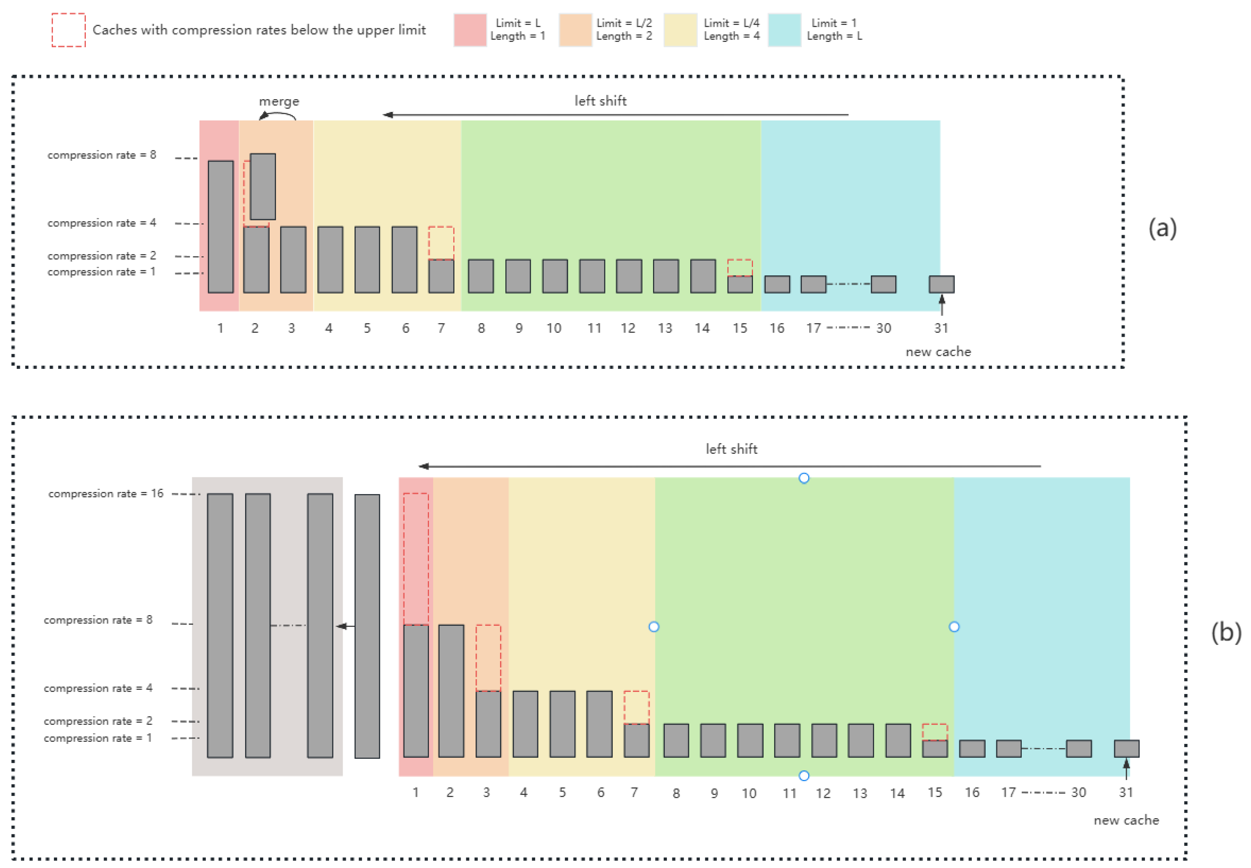
To implement this, we propose a distance-based compression method. Specifically, we determine their upper compression ratio limit based on their distance from the token generation location and the hyperparameter $L=2^k$. The upper limit of the compression ratio for each cache unit is illustrated in Figure 1, where the different cache groups and their corresponding compression limits are shown. Ordered by proximity to the next token, the first group of cache units has an upper limit of 1, and the number of units is L. The second group has an upper limit of 2, and the number of units is ${\displaystyle \frac{L}{2}}$. This pattern continues, with each subsequent group doubling the compression ratio limit and halving the number of units compared to the previous group, until the number reaches 1, at which point the compression ratio limit is L. Based on this, our method dynamically adjusts and merges the cache during the inference process.

3.1. Merge Planning

In the inference process, effective cache management and compression are critical for ensuring optimal performance. We adopt a priority strategy based on the compression ratio r: cache units with the lowest r are compressed first, to avoid excessive compression of higher-r units that could cause severe information loss. When multiple cache units share the same compression ratio, we prioritize the one farthest from the next predicted token.

To rigorously characterize the compression and merge process, we define the input sequence length as n, the number of Transformer layers as $L_{\mathrm{layer}}$, the number of attention heads per layer as H, and the key/value dimensions as $d_k$ and $d_v$, respectively. In the l-th layer and h-th head at time step t, the key and value are denoted by $K_t^{(l,h)}\in {\mathbb{R}}^{d_k}$ and $V_t^{(l,h)}\in {\mathbb{R}}^{d_v}$. A cache unit ${\mathcal{U}}_t$ is defined as the set of all $(K,V)$ pairs at the same time step across all layers and heads:

$${\mathcal{U}}_t\triangleq \left\{(K_t^{(l,h)},V_t^{(l,h)})|l=1,\dots ,L_{\mathrm{layer}},h=1,\dots ,H\right\}.$$

(1)

The compression ratio $r\in \mathbb{N}$ denotes the number of original tokens represented by a single cache unit. If a compressed unit $\tilde{\mathcal{U}}$ represents r consecutive tokens, then its compression ratio is r.

For a single-head attention with query q, using an uncompressed history ${\mathcal{H}}_i={\left\{(K_t,V_t)\right\}}_{t\le i}$, the output is

$$\mathrm{Attn}(q;{\mathcal{H}}_i)\triangleq \sum _{t\le i}{\alpha }_t\left(q\right)V_t,{\alpha }_t\left(q\right)={\displaystyle \frac{exp\left(\frac{q^{\top }{K}_t}{\sqrt{d_k}}\right)}{{\sum }_{s\le i}exp\left(\frac{q^{\top }{K}_s}{\sqrt{d_k}}\right)}}.$$

(2)

After compression, with the representative set ${\tilde{\mathcal{H}}}_i={\left\{({\tilde{K}}_u,{\tilde{V}}_u,r_u)\right\}}_u$ where $r_u$ denotes the number of tokens represented, the attention output becomes

$$\widetilde{\mathrm{Attn}}(q;{\tilde{\mathcal{H}}}_i)\triangleq \sum _u{\tilde{\alpha }}_u\left(q\right){\tilde{V}}_u,{\tilde{\alpha }}_u\left(q\right)={\displaystyle \frac{exp\left(\frac{q^{\top }{\tilde{K}}_u}{\sqrt{d_k}}\right)}{{\sum }_{v}exp\left(\frac{q^{\top }{\tilde{K}}_v}{\sqrt{d_k}}\right)}}.$$

(3)

The information loss is measured as

$${\mathcal{L}}_{\mathrm{IL}}\triangleq {\mathbb{E}}_q\left[\parallel \mathrm{Attn}(q;{\mathcal{H}}_i)-\widetilde{\mathrm{Attn}}(q;{\tilde{\mathcal{H}}}_i){\parallel }_2^2\right],$$

(4)

representing the expected squared deviation between the attention outputs with full and compressed histories.

To manage caches, we define two queues: the far queue $Q_1$ and the near queue $Q_2$. $Q_1$ stores cache units that no longer require compression and have no length restriction, allowing long-term storage. $Q_2$ stores cache units that require compression, with a maximum length constraint

$$|Q_2|\le L_{\max }=2\times L_{\mathrm{group}}-1,$$

(5)

where $L_{\mathrm{group}}$ is a grouping parameter independent of the number of Transformer layers $L_{\mathrm{layer}}$. During token prediction, the merged queue

$$Q=Q_1+Q_2$$

(6)

forms the historical context ${\mathcal{H}}_i$ used in attention computation.

As new caches are generated, if $Q_2$ reaches its capacity, a systematic merging process is performed. Starting from the head of $Q_2$, we locate the first cache unit whose compression ratio r has not reached its upper limit. We then find the cache unit closest to the tail of $Q_2$ with the same compression ratio and merge it with its preceding cache unit. If all cache units in $Q_2$ have reached their compression limits, the cache unit at the tail of $Q_2$ is moved to $Q_1$. After either merging or transferring, the newly generated cache unit is appended to $Q_2$.

For each new token, the following process is carried out:

• If $|Q_2|<2\times L_{\mathrm{group}}-1$, enqueue the new $\mathcal{U}$;
• Otherwise, apply $f\left(p\right)$ for the earliest unsatisfied $p\in \mathcal{P}$;
• If all positions meet their limits, the tail of $Q_2$ is moved to $Q_1$, and the process restarts from $f\left(1\right)$.

During the extensive inference process of large models, the continuous computation of merge positions introduces a significant temporal overhead. However, upon closer examination, a pattern in the compression scheme becomes apparent, revealing that the real-time calculation of merge positions is, in fact, unnecessary during inference. Instead, it is possible to precompute all merge positions before the actual inference begins, thereby eliminating the need for ongoing calculations during runtime.

The queue of merge positions can be divided into two distinct segments, each corresponding to a specific phase in the overall merge pattern. The first segment occurs when no cache has yet been moved to the $Q_1$ queue. The second segment, on the other hand, occurs when all cache units have reached their maximum compression ratios. At this stage, the cache unit at the tail of the queue is moved to the $Q_1$, and this process continues until every cache unit has again reached the upper limit of its compression ratio. The subsequent stages of inference rely exclusively on this second segment of the merge process, ensuring that once the initial phase is complete, the remaining merge positions follow a predictable, repetitive pattern. This cyclical process eliminates the need for real-time computation and ensures that the entire merge procedure is efficiently handled before inference commences.

As shown in Figure 2 for the case $L_{\mathrm{group}}=16$, certain positions within the inference process are of particular importance, referred to as key positions. These are located at the rightmost boundary of groups whose compression upper limit is greater than 1. When a merge operation is executed at a specific key position, the resulting leftward shift implies that all subsequent key positions to the right of the current merge position will also require merge operations to maintain their compression upper limits.

Let the positions in $Q_2$ be indexed from nearest to farthest as $1,2,\dots ,2\times L_{\mathrm{group}}-1$. An algorithm precomputes the sequence of key positions:

$$\mathcal{P}=\{p_1,p_2,\dots ,p_m\},p_i=2^i-1,p_i\le 2\times L_{\mathrm{group}}-1.$$

(7)

The merge-scheduling operator $f\left(p\right)$ for a key position p is defined recursively:

• First, invoke $f(2\times p+1)$, ensuring merges at more distant key positions are performed before handling p;
• At position p, perform a merge and record it via $recordPosition\left(p\right)$;
• Invoke $f(2\times p+1)$ again to ensure that, after processing p, all further positions still satisfy the compression schedule.

The computation of merge positions in the first part can be implemented as Algorithm 1:

Algorithm 1 Merge scheduling for first segment

1: Input: Queue $Q_2$, $L_{\mathrm{group}}$ 2: $i\leftarrow L_{\mathrm{group}}$ 3: while  $i>0$  do 4:    for $j=1$ to $i-1$ do 5:      $recordPosition\left(j\right)$ 6:      $f(2\times j+1)$ 7:    end for 8:    $i\leftarrow i/2$ 9: end while

For the second part, when all units have reached their upper limits, the tail element of $Q_2$ is moved into $Q_1$, and the process restarts from $f\left(1\right)$.

In a steady state, the $(2L_{\mathrm{group}}-1)$ representative units in $Q_2$ collectively cover approximately

$$T_{Q_2}\left(L_{\mathrm{group}}\right)=\sum _{g=0}^k{\displaystyle \frac{L_{\mathrm{group}}}{2^g}}·2^g=L_{\mathrm{group}}(k+1)=L_{\mathrm{group}}\left(1+{log}_2{L}_{\mathrm{group}}\right)$$

(8)

tokens. Given a total context length n, the remaining distant tokens are summarized into $Q_1$ at ratio $L_{\mathrm{group}}$, yielding an effective number of units per step of

$$N_{\mathrm{eff}}(n,L_{\mathrm{group}})\approx (2L_{\mathrm{group}}-1)+max\left\{0,⌈{\displaystyle \frac{n-T_{Q_2}\left(L_{\mathrm{group}}\right)}{L_{\mathrm{group}}}}⌉\right\}.$$

(9)

This determines the retrieval cost in attention computation and the KV read bandwidth, scaling with slope $1/L_{\mathrm{group}}$ for $n\gg L_{\mathrm{group}}log{L}_{\mathrm{group}}$.

3.2. Merge Model

The core of our method lies in a merge model designed to minimize information loss during compression of cache units. Simple approaches such as linear averaging may discard high-order semantic interactions. To address this, we introduce a trainable multilayer perceptron (MLP) as the merge operator,

$$M_{\theta }:({\mathcal{U}}_a,{\mathcal{U}}_b)\mapsto {\mathcal{U}}_{a\oplus b},$$

(10)

which performs nonlinear fusion of adjacent cache units ${\mathcal{U}}_a$ and ${\mathcal{U}}_b$ corresponding to segments ${\mathcal{S}}_a$ and ${\mathcal{S}}_b$. The objective is

$$\forall q:\mathrm{Attn}\left(q;\mathcal{H}\cup \{{\mathcal{U}}_a,{\mathcal{U}}_b\}\right)\approx \mathrm{Attn}\left(q;\mathcal{H}\cup \left\{M_{\theta }({\mathcal{U}}_a,{\mathcal{U}}_b)\right\}\right).$$

(11)

The training objective combines

$$\begin{array}{cc}\hfill {\mathcal{L}}_{\mathrm{IL}}\left(\theta \right)& ={\mathbb{E}}_q\left[\parallel \mathrm{Attn}(q;\mathcal{H}\cup \{{\mathcal{U}}_a,{\mathcal{U}}_b\})-\mathrm{Attn}(q;\mathcal{H}\cup \left\{M_{\theta }({\mathcal{U}}_a,{\mathcal{U}}_b)\right\}){\parallel }_2^2\right],\hfill \end{array}$$

(12)

$$\begin{array}{cc}\hfill {\mathcal{L}}_{\mathrm{align}}\left(\theta \right)& =\mathbb{E}\left[\parallel h_{i+1}^{\mathrm{full}}-h_{i+1}^{\mathrm{comp}}{\parallel }_2^2\right]+\lambda ·\mathrm{KL}\left(p^{\mathrm{full}}(·|x)\parallel p^{\mathrm{comp}}(·|x)\right),\hfill \end{array}$$

(13)

along with regularization to constrain magnitude and preserve scale invariance of K.

The choice of an MLP is motivated by both efficiency and theoretical considerations: as a universal approximator, it can model any continuous function on a compact domain [29], capturing complex nonlinear interactions between cache units while remaining computationally lightweight. More expressive architectures, such as self-attention-based models, could be used but incur substantial computational and memory costs, especially given the high frequency of merge operations.

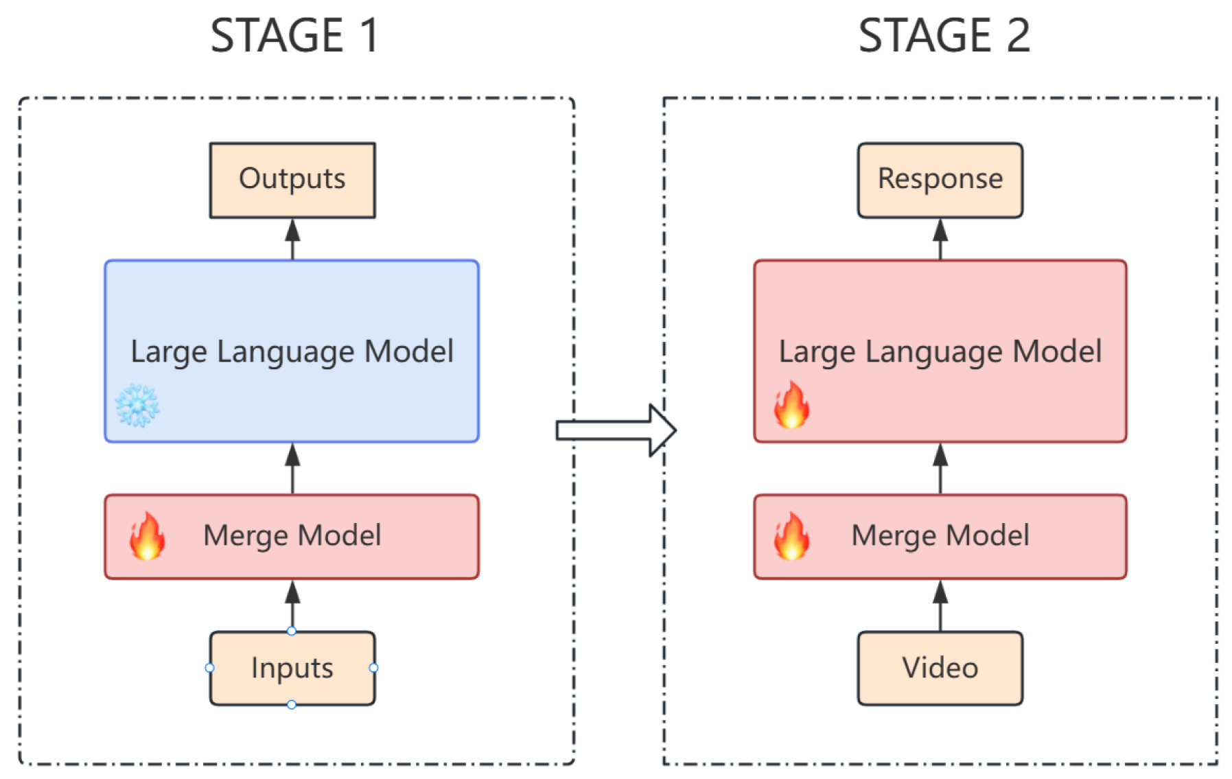
To mitigate potential semantic drift—i.e., the mismatch between merged cache representations and the distribution that the LLM was trained on—we suggest a two-stage training procedure. First, the merge model is trained to produce semantically faithful cache representations. Optionally, the LLM can be fine-tuned to better adapt to these compressed representations, thereby improving robustness and inference quality.

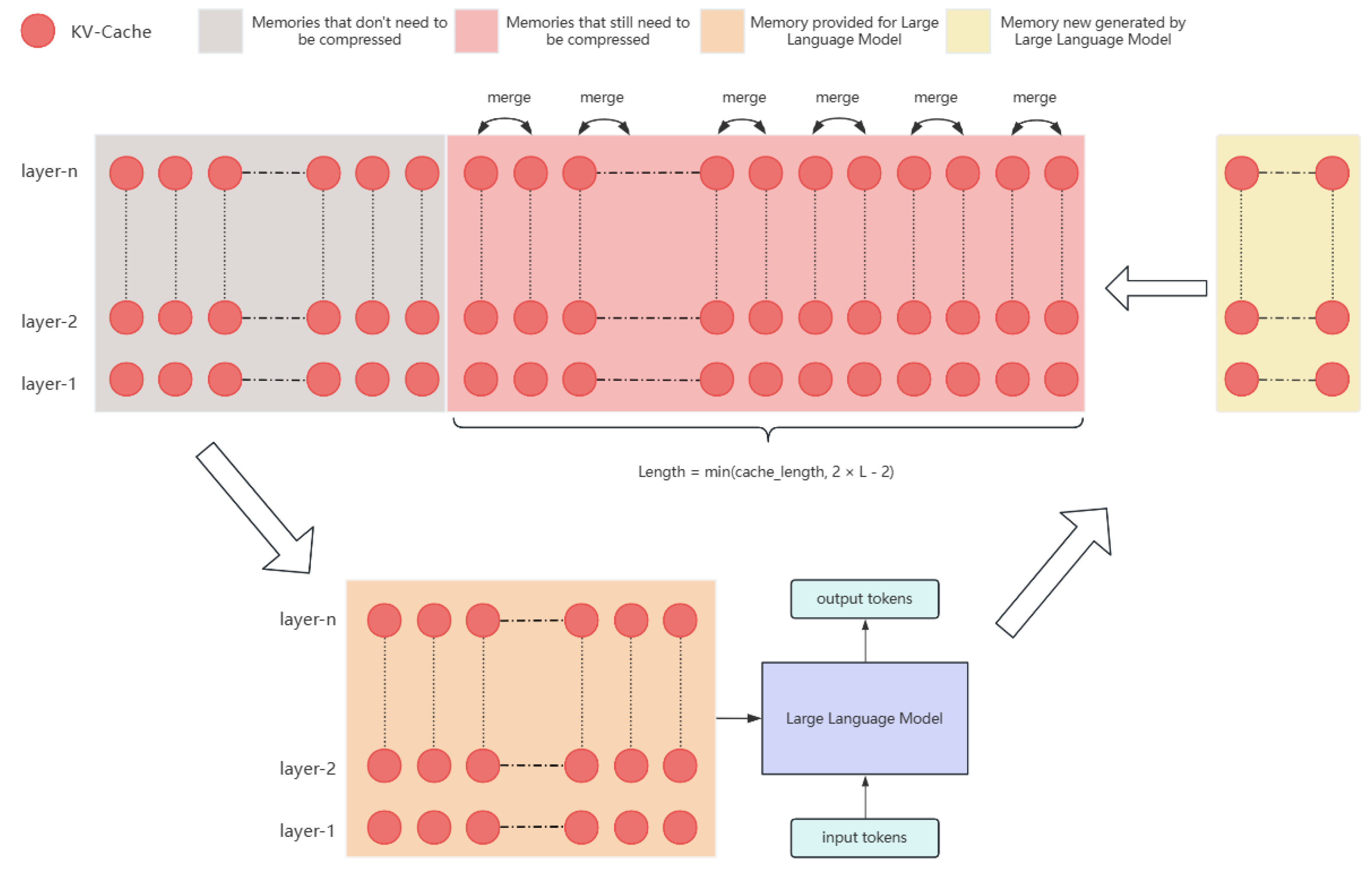
During training, to maintain efficiency, we adopt a chunk-based merge strategy: multiple tokens are grouped into a single compression unit, and the merge operation is applied per chunk rather than token by token. This contrasts with stepwise merging during inference and significantly improves training throughput. Figure 3 illustrates the simplified compression structure used in training. The overall training pipeline, depicted in Figure 4, consists of first training the merge model and then optionally fine-tuning the LLM to align with the merged representations.

4. Experiment

4.1. Datasets

LongBench v2 [20] serves as a comprehensive benchmark designed to evaluate the ability of LLMs in understanding and processing extended texts. LongBench v2 is structured into six primary categories, comprising twenty distinct tasks, which encompass critical long-text application scenarios such as Single-Doc QA, Multi-Doc QA, Long ICL, Dialogue History, Code Repo, and Structured Data.

4.2. Hyperparameter Selection

In the hyperparameter selection phase, the primary objective is to evaluate the model’s performance across a range of hyperparameter configurations in a systematic and efficient manner. This process aims to identify the optimal set of hyperparameters that maximizes model performance while minimizing computational overhead. By exploring various combinations of hyperparameters, the goal is to balance trade-offs between accuracy, generalization, and resource utilization, ultimately improving the model’s robustness and efficiency.

4.2.1. MLP Layer Depths

We utilize a standard MLP to integrate distinct cache layers, driven by the hypothesis that two cache instances can be effectively combined to form a unified cache that the LLMs can interpret. This hypothesis appears to be intuitive, as utilizing MLPs for extracting and integrating information is a common practice in the field of deep learning. However, the challenge lies in whether caches with different layers and compression ratios can indeed be merged without significant loss of performance. To explore this, we implemented MLPs with varying layer configurations and monitored the LLMs’ performance after cache compression. This allowed us to assess the optimal MLP configuration for cache integration. If the results suggest suboptimal performance, it may indicate the necessity for a separate MLP for each cache layer. Moreover, even a simple MLP might not suffice for this task, highlighting the potential complexity involved in cache merging.

The experimental results, as shown in

Table 1. Predicted performance of the Llama-3.1-8B-Instruct model as a base model, with merge models of varying MLP layer depths, on the Qasper, MultiFieldQA-en, and 2WikiMultihopQA datasets.

Layer	Qasper	MultiFieldQA-en	2WikiMultihopQA
3	38.5	28.5	42.0
6	44.0	34.0	48.5
9	46.5	35.5	50.0
12	47.0	37.0	51.5
15	48.5	38.5	53.0
18	47.0	39.0	52.0

, are promising. They demonstrate that a single, standard MLP is capable of successfully merging caches from some layer configuration, which aligns with the objectives of our assumptions. This outcome suggests that, contrary to initial concerns, the integration process can be achieved efficiently with a single MLP, without the need for additional layer-specific models.

4.2.2. Group Length

The impact of $L_1$ and $L_2$ on accuracy is summarized in

Table 2. Predicted accuracy of the Llama-3.1-8B-Instruct model as a base model, with a 9-layer MLP merge model, on the Single-Doc QA, Multi-Doc QA and Few-Shot Learning, using hyperparameters $L=L_1$ during training and $L=L_2$ during testing.

	$L_2$	4	8	16	32	64	128	256	512
$L_1$
4		32.8	29.3	30.7	25.6	20.3	15.8	13.5	10.2
8		31.7	29.9	27.1	24.5	22.1	16.9	12.8	9.8
16		33.0	32.0	28.3	22.0	21.4	15.2	11.4	9.0
32		34.6	31.8	31.8	28.2	18.0	13.3	10.0	7.6
64		30.3	31.3	32.4	29.6	24.4	14.5	12.3	8.7
128		29.6	30.8	32.9	26.7	25.1	19.8	11.0	9.3
256		29.5	29.9	31.7	27.1	26.3	20.0	14.2	10.8
512		34.0	31.5	29.0	26.0	28.0	30.0	32.0	33.8
(a) Predicted accuracy on the Single-Doc QA.
	$L_2$	4	8	16	32	64	128	256	512
$L_1$
4		24.1	18.5	18.7	15.3	14.6	10.7	9.8	8.1
8		23.0	19.8	19.4	15.9	15.1	11.5	8.9	6.5
16		23.2	22.1	20.6	17.3	16.2	12.4	10.1	7.2
32		25.1	23.7	23.5	18.8	17.5	13.3	9.5	6.8
64		24.6	23.9	24.4	20.0	18.8	14.3	11.6	8.0
128		24.8	24.2	25.7	21.5	19.5	16.2	12.0	9.4
256		24.9	24.3	25.9	22.0	20.3	16.8	13.5	9.5
512		25.2	24.0	23.2	21.0	21.5	23.0	23.8	24.1
(b) Predicted accuracy on the Multi-Doc QA.
	$L_2$	4	8	16	32	64	128	256	512
$L_1$
4		60.4	54.0	54.8	48.6	36.6	20.5	20.2	15.0
8		65.2	55.7	54.1	48.5	39.0	26.5	15.4	10.2
16		64.4	60.9	56.0	46.8	36.8	22.6	17.0	12.1
32		63.0	61.5	62.4	52.0	36.6	20.5	14.8	11.0
64		62.4	62.2	62.5	55.0	47.0	26.0	21.0	15.6
128		61.8	62.4	63.7	54.7	46.0	36.8	20.2	18.5
256		63.0	60.8	62.4	55.7	45.8	37.7	23.3	20.4
512		65.2	62.0	60.0	54.0	55.0	58.5	61.0	65.4
(c) Predicted accuracy for Few-Shot Learning.

. In our experiments, increasing $L_1$ generally does not degrade accuracy, although it does not always lead to improvements. In contrast, when $L_2>L_1$, accuracy drops significantly. Within the range $L_2\le L_1$, accuracy first declines and then gradually recovers as $L_2$ increases. The observed accuracy drop manifests not only as incorrect answers but occasionally as the generation of meaningless content, suggesting that LLMs may struggle to fully interpret caches compressed via MLPs. Possible contributing factors include limited MLP capacity, insufficient training, or the potential need for model fine-tuning to accommodate compressed caches.

Interestingly, simply setting $L_1=L_2$ does not guarantee improved accuracy. Larger $L_1$ values sometimes lead to higher accuracy, particularly when $L_2$ is also large. This indicates that models trained with higher $L_1$ can better adapt to higher compression ratios. If this hypothesis holds, it implies that a single general-purpose model trained with a sufficiently large L can accommodate a range of L values at inference, without the need for separate models for each configuration.

We conduct a detailed sensitivity study by varying L across a wide range of values. We evaluate model accuracy relative to the reference setting $L=512$ (denoted as $\Delta$) and simultaneously measure the information loss ${\mathcal{L}}_{\mathrm{IL}}$. A positive $\Delta$ indicates accuracy degradation compared with the baseline $L=512$.

Overall, the curves in Figure 5 indicate that smaller L values generally reduce ${\mathcal{L}}_{\mathrm{IL}}$ and improve task accuracy. In contrast, when L becomes larger, the risk of over-compression effects and reduced alignment with the trained merge distribution leads to increased information loss (${\mathcal{L}}_{\mathrm{IL}}$) and lower accuracy. Nevertheless, the overall trend tends to flatten as L continues to increase.

Empirically, when L is small, our method behaves similarly to a Compressive Transformer: the compression ratio is low, resulting in minimal information loss but also limited performance gains. The uncompressed window in this regime is smaller than that of a standard Compressive Transformer. When L is large, distant caches are highly compressed, while the low-compression region expands, effectively acting as a sliding window. Compared to a conventional sliding window, our approach retains more information in the low-compression region and preserves distant information in a highly compressed form. The former improves memory efficiency, while the latter can be advantageous or detrimental depending on whether the model can extract meaningful signals from highly compressed caches.

The steady-state effective unit count can be approximated as

$$N_{\mathrm{eff}}(n,L)\approx (2L-1)+max\left\{0,⌈{\displaystyle \frac{n-L(1+{log}_{2}L)}{L}}⌉\right\}.$$

(14)

If the design objective is to minimize a combination of error and cost,

$$\underset{L}{min}E\left(L\right)+\mu ·N_{\mathrm{eff}}(n,L),$$

(15)

where $E\left(L\right)$ decreases with L and can be modeled as $E\left(L\right)\approx {\displaystyle \frac{c_1}{logL}}$—reflecting that the effective coverage $T_{Q_2}\propto LlogL$ grows with L—and the dominant cost term is $c_{2}L+c_{3}n/L$. The first-order condition yields

$$L^{★}\asymp \sqrt{n},$$

(16)

neglecting the slowly varying $logL$ factor. This provides a theoretical rationale for the empirical rule that L should scale with the square root of the context length.

In practice, we recommend setting

$$L=\sqrt{\mathrm{sentence\_length}+\mathrm{max\_token}}$$

(17)

as a heuristic choice for the hyperparameter. This balances compression efficiency and accuracy, allowing the model to retain sufficient context while keeping memory usage manageable.

Future work may explore the adaptive selection of L based on the semantic importance of tokens or cache units, potentially improving performance without increasing computational cost.

4.3. Quality, Stability, and Efficiency of Hierarchical Cache Compression

We evaluate the quality and stability of cache compression using three metrics: information loss, semantic drift, and boundary discontinuity. The information loss metric is defined as

$${\mathcal{L}}_{\mathrm{IL}}={\mathbb{E}}_q\left[\parallel \mathrm{Attn}(q;{\mathcal{H}}_i)-\widetilde{\mathrm{Attn}}(q;{\tilde{\mathcal{H}}}_i){\parallel }_2^2\right],$$

(18)

computed over a sampled set of queries q at each decoding step and averaged across layers. Semantic drift is quantified using the Semantic Drift Index (SDI):

$$\mathrm{SDI}\triangleq \alpha ·\left(1-cos(h^{\mathrm{full}},h^{\mathrm{comp}})\right)+(1-\alpha )·\mathrm{JS}\left({\alpha }^{\mathrm{full}},{\alpha }^{\mathrm{comp}}\right),$$

(19)

where ${\alpha }^{\mathrm{full}}$ and ${\alpha }^{\mathrm{comp}}$ are attention weight distributions, and $\mathrm{JS}$ denotes Jensen–Shannon divergence. Lower SDI values indicate higher semantic stability. Boundary Semantic Discontinuity (BSD) measures discontinuities at block boundaries:

$$\mathrm{BSD}\triangleq {\displaystyle \frac{1}{Z}}\sum _{\mathrm{boundaries}b}\parallel {\alpha }_{b-ϵ}-{\alpha }_{b+ϵ}{\parallel }_1,$$

(20)

where $ϵ$ is a small step radius and Z is a normalization factor.

During training, compression is applied per block, while inference uses multi-level hierarchical merging. To reduce distribution shift and BSD, we propose the following: (A) Train-As-Inference (TAI), simulating the inference-time binary merge schedule within each block; (B) boundary regularization, adding a penalty $\gamma ·\mathrm{BSD}$ to encourage continuity across block edges.

We evaluate ${\mathcal{L}}_{\mathrm{IL}}$, SDI, and BSD on Single-Doc QA (9-layer MLP, $L=512$, block length 128).

Table 3. Baseline metrics for Single-Doc QA and improvements from TAI and boundary regularization.

Method	${\mathcal{L}}_{\mathbf{IL}}$	SDI	BSD
Baseline	0.13	0.10	0.065
TAI only	0.12	0.10	0.048
TAI + Boundary Reg.	0.11	0.08	0.041

summarizes baseline results and the improvements from Train-As-Inference (TAI) and boundary regularization.

For $L=512$, TAI reduces BSD from 0.065 to 0.048 and ${\mathcal{L}}_{\mathrm{IL}}$ from 0.13 to 0.12; combining both techniques further reduces BSD to 0.041 and ${\mathcal{L}}_{\mathrm{IL}}$ to 0.11.

Efficiency is measured via per-step latency $t_{\mathrm{step}}$, peak memory $M_{\mathrm{peak}}$, energy consumption E, KV bytes per unit $B_{\mathrm{KV}}$, and effective unit count $N_{\mathrm{eff}}(n,L)$. Memory compression ratio is computed as

$${\mathcal{C}}_M(n,L)\approx {\displaystyle \frac{n}{(2L-1)+max\{0,\lceil (n-L(1+{log}_{2}L))/L\rceil \}}}.$$

(21)

Table 4. Computational efficiency and memory usage for different L values.

Configuration	${\mathit{t}}_{\mathbf{step}}$ (ms)	${\mathit{M}}_{\mathbf{peak}}$ (GB)	E (J/1k Tokens)	${\mathit{N}}_{\mathbf{eff}}$
Uncompressed	38.5	46	118	${10}^5$
$L=512$	3.9	6.1	15	1208
$L=256$	5.6	8.7	21	1357

presents representative values for $n={10}^5$ tokens on an A100 80GB GPU in BF16 precision.

Compared to uncompressed inference, $L=512$ achieves ∼$82.8\times$ memory compression, ∼$10\times$ faster per-step latency, and ∼$8\times$ lower energy consumption. Memory growth follows $O\left((2L-1)+n/L\right)$, with constant per-step merge cost due to precomputed positions. Our method is deterministic, in contrast to other architectures such as Compressive Transformer, Infini-attention, or InfLLM, which have varying degrees of determinism and memory growth patterns.

To account for differences in backbone strength, we normalize scores

$$S_{\mathrm{norm}}={\displaystyle \frac{S_{\mathrm{method}}}{S_{\mathrm{base}}}},$$

(22)

yielding 1.02, 1.05, and 1.01 for Single-Doc QA, Multi-Doc QA, and Few-Shot tasks, respectively.

4.4. Prediction Accuracy

To evaluate the accuracy of our method on long-context tasks, we conducted experiments using our model on the Longbench v2 dataset. The results were then compared with mainstream LLMs such as GLM-4-9B-Chat and Qwen2.5-72B-Inst [30]. As shown in

Table 5. Predicted accuracy of the Llama-3.1-8B-Instruct model as a base model, when the merge model is composed of a 9-layer MLP, is evaluated across 6 tasks: I. Single-Doc QA, II. Multi-Doc QA, III. Long ICL, IV. Dialogue History, V. Code Repo, and VI. Structured Data, with hyperparameters $L=512$. The best results are highlighted in bold.

	Avg	I	II	III	IV	V	VI
GLM-4-9B-Chat	30.2	30.9	27.2	33.3	38.5	28.0	24.2
GLM-4-Plus	44.3	41.7	42.4	46.9	51.3	46.0	48.5
Qwen2.5-72B-Inst.	39.4	40.6	35.2	42.0	25.6	50.0	42.4
GPT-4o	50.1	48.6	44.0	58.0	46.2	56.0	51.5
Llama-3.1-8B-Inst.	30.0	34.9	30.4	23.5	17.9	32.0	30.3
Our method(Llama-3.1-8B-Inst.)	35.6	35.8	36.1	38.2	37.4	39.3	28.0

, our model achieves accuracy close to GLM-4-9B-Chat with the hyperparameter setting of $L=512$. However, considering that our base model Llama-3.1-8B-Instruct already has a stronger capability in handling long contexts, the results are not particularly surprising.

5. Conclusions

Our method proposes a distance-based compression method based on the idea of a Compressive Transformer, which realizes more flexible compression ratio control with a simple compression method, and saves computational cost, while the accuracy is close to that of the original model. However, our method still has limitations. It heavily relies on two components: a merge model that can combine KV-caches with minimal information loss, and an LLM capable of effectively interpreting the compressed KV-cache. Both components currently lack theoretical foundations and efficient training methodologies.

References

1. Vaswani, A. Attention is all you need. Adv. Neural Inf. Process. Syst. 2017, 30, 5998–6008. [Google Scholar]
2. Learning long-term dependencies with gradient descent is difficult. IEEE Trans. Neural Netw. 1994, 5, 157–166. [CrossRef] [PubMed]
3. Radford, A.; Kim, J.W.; Hallacy, C.; Ramesh, A.; Goh, G.; Agarwal, S.; Sastry, G.; Askell, A.; Mishkin, P.; Clark, J.; et al. Learning transferable visual models from natural language supervision. In Proceedings of the International Conference on Machine Learning PMLR, Virtual, 18–24 July 2021; pp. 8748–8763. [Google Scholar]
4. Wei, J.; Wang, X.; Schuurmans, D.; Bosma, M.; Xia, F.; Chi, E.; Le, Q.V.; Zhou, D. Chain-of-thought prompting elicits reasoning in large language models. Adv. Neural Inf. Process. Syst. 2022, 35, 24824–24837. [Google Scholar]
5. Child, R.; Gray, S.; Radford, A.; Sutskever, I. Generating long sequences with sparse transformers. arXiv 2019, arXiv:1904.10509. [Google Scholar] [CrossRef]
6. Beltagy, I.; Peters, M.E.; Cohan, A. Longformer: The long-document transformer. arXiv 2020, arXiv:2004.05150. [Google Scholar] [CrossRef]
7. Kitaev, N.; Kaiser, Ł.; Levskaya, A. Reformer: The efficient transformer. arXiv 2020, arXiv:2001.04451. [Google Scholar] [CrossRef]
8. Wang, S.; Li, B.Z.; Khabsa, M.; Fang, H.; Ma, H. Linformer: Self-attention with linear complexity. arXiv 2020, arXiv:2006.04768. [Google Scholar] [CrossRef]
9. Zaheer, M.; Guruganesh, G.; Dubey, K.A.; Ainslie, J.; Alberti, C.; Ontanon, S.; Pham, P.; Ravula, A.; Wang, Q.; Yang, L.; et al. Big bird: Transformers for longer sequences. Adv. Neural Inf. Process. Syst. 2020, 33, 17283–17297. [Google Scholar]
10. Dai, Z. Transformer-xl: Attentive language models beyond a fixed-length context. arXiv 2019, arXiv:1901.02860. [Google Scholar]
11. Rae, J.W.; Potapenko, A.; Jayakumar, S.M.; Lillicrap, T.P. Compressive transformers for long-range sequence modelling. arXiv 2019, arXiv:1911.05507. [Google Scholar] [CrossRef]
12. Munkhdalai, T.; Faruqui, M.; Gopal, S. Leave no context behind: Efficient infinite context transformers with infini-attention. arXiv 2024, arXiv:2404.07143. [Google Scholar] [CrossRef]
13. Xiao, C.; Zhang, P.; Han, X.; Xiao, G.; Lin, Y.; Zhang, Z.; Liu, Z.; Han, S.; Sun, M. Infllm: Unveiling the intrinsic capacity of llms for understanding extremely long sequences with training-free memory. arXiv 2024, arXiv:2402.04617. [Google Scholar]
14. Brown, T.; Mann, B.; Ryder, N.; Subbiah, M.; Kaplan, J.D.; Dhariwal, P.; Neelakantan, A.; Shyam, P.; Sastry, G.; Askell, A.; et al. Language models are few-shot learners. Adv. Neural Inf. Process. Syst. 2020, 33, 1877–1901. [Google Scholar]
15. Raffel, C.; Shazeer, N.; Roberts, A.; Lee, K.; Narang, S.; Matena, M.; Zhou, Y.; Li, W.; Liu, P.J. Exploring the limits of transfer learning with a unified text-to-text transformer. J. Mach. Learn. Res. 2020, 21, 1–67. [Google Scholar]
16. Devlin, J.; Chang, M.W.; Lee, K.; Toutanova, K. Bert: Pre-training of deep bidirectional transformers for language understanding. In Proceedings of the 2019 Conference of the North American Chapter of the Association for Computational Linguistics: Human Language Technologies, Minneapolis, MN, USA, 2–7 June 2019; Volume 1, pp. 4171–4186. [Google Scholar]
17. Rajpurkar, P. Squad: 100,000+ questions for machine comprehension of text. arXiv 2016, arXiv:1606.05250. [Google Scholar]
18. Zhang, Y. Dialogpt: Large-Scale generative pre-training for conversational response generation. arXiv 2019, arXiv:1911.00536. [Google Scholar]
19. Tay, Y.; Dehghani, M.; Abnar, S.; Shen, Y.; Bahri, D.; Pham, P.; Rao, J.; Yang, L.; Ruder, S.; Metzler, D. Long range arena: A benchmark for efficient transformers. arXiv 2020, arXiv:2011.04006. [Google Scholar] [CrossRef]
20. Bai, Y.; Tu, S.; Zhang, J.; Peng, H.; Wang, X.; Lv, X.; Cao, S.; Xu, J.; Hou, L.; Dong, Y.; et al. Longbench v2: Towards deeper understanding and reasoning on realistic long-context multitasks. arXiv 2024, arXiv:2412.15204. [Google Scholar]
21. Li, T.; Zhang, G.; Do, Q.D.; Yue, X.; Chen, W. Long-context llms struggle with long in-context learning. arXiv 2024, arXiv:2404.02060. [Google Scholar]
22. Zhang, X.; Chen, Y.; Hu, S.; Xu, Z.; Chen, J.; Hao, M.K.; Han, X.; Thai, Z.L.; Wang, S.; Liu, Z.; et al. Bench: Extending Long Context Evaluation Beyond 100K Tokens. arXiv 2024, arXiv:2402.13718. [Google Scholar]
23. Wu, Y.; Rabe, M.N.; Hutchins, D.; Szegedy, C. Memorizing transformers. arXiv 2022, arXiv:2203.08913. [Google Scholar] [CrossRef]
24. Chandar, S.; Ahn, S.; Larochelle, H.; Vincent, P.; Tesauro, G.; Bengio, Y. Hierarchical memory networks. arXiv 2016, arXiv:1605.07427. [Google Scholar] [PubMed]
25. Wu, Y.; Zhao, Y.; Hu, B.; Minervini, P.; Stenetorp, P.; Riedel, S. An efficient memory-augmented transformer for knowledge-intensive nlp tasks. arXiv 2022, arXiv:2210.16773. [Google Scholar]
26. Su, J.; Ahmed, M.; Lu, Y.; Pan, S.; Bo, W.; Liu, Y. Roformer: Enhanced transformer with rotary position embedding. Neurocomputing 2024, 568, 127063. [Google Scholar] [CrossRef]
27. Xiong, W.; Liu, J.; Molybog, I.; Zhang, H.; Bhargava, P.; Hou, R.; Martin, L.; Rungta, R.; Sankararaman, K.A.; Oguz, B.; et al. Effective long-context scaling of foundation models. arXiv 2023, arXiv:2309.16039. [Google Scholar] [CrossRef]
28. Chen, S.; Wong, S.; Chen, L.; Tian, Y. Extending context window of large language models via positional interpolation. arXiv 2023, arXiv:2306.15595. [Google Scholar] [CrossRef]
29. Hornik, K.; Stinchcombe, M.; White, H. touvron2023llama. Neural Netw. 1989, 2, 359–366. [Google Scholar] [CrossRef]
30. Yang, A.; Li, A.; Yang, B.; Zhang, B.; Hui, B.; Zheng, B.; Yu, B.; Gao, C.; Huang, C.; Lv, C.; et al. Qwen3 technical report. arXiv 2025, arXiv:2505.09388. [Google Scholar] [CrossRef]
Figure 1. This illustration demonstrates the upper limit of the compression ratio, with different colors used to represent different groups. As the cache unit approaches the next token, its compression ratio decreases. To simplify the inference process, each group’s upper limit is doubled and the number of units halved compared to the previous group, ensuring the product of the upper limit and the number of units remain constant at hyperparameter L. The light gray on the far left represents the cache units moved into Q 1 , with a quantity of m.
Applsci 15 09482 g001
Figure 2. Illustration of the two distinct cases that occur during the compression process. (a) The first case occurs before any cache is moved into Q 1 , where the length of Q 2 is maintained at 2 × L 1 through constant compression while new caches are added. (b) The second case occurs after a cache from Q 2 has been moved into Q 1 , where some caches in Q 2 have not yet reached the upper limit of the compression ratio and still need to be compressed following the move.
Applsci 15 09482 g002
Figure 3. Illustration of the compression method during the training phase. As depicted, the compression in the training phase only requires pairwise compression of the cache units on the right side.
Applsci 15 09482 g003
Figure 4. Illustration of the training process. The first stage is to train the merge model so that it can retain as much information as possible when compressing the cache. The second stage is to fine-tune the LLM and merge model so that the LLM correctly understands the compressed cache.
Applsci 15 09482 g004
Figure 5. Sensitivity curves under varying L. (a) Relative change Δ : positive values mean performance degradation. (b) Information loss L IL : lower values indicate closer approximation to the full-attention model.
Applsci 15 09482 g005