Article

Machine Learning-Based Predictive Modeling for Solid Oxide Electrolysis Cell (SOEC) Electrochemical Performance

by
Nathan Gil A. Estrada
1,* and
Rinlee Butch M. Cervera
2,*
1
Energy Engineering Graduate Program, University of the Philippines Diliman, Quezon City 1101, Philippines
2
Energy Storage and Conversion Materials Laboratory, Department of Mining, Metallurgical, and Materials Engineering, University of the Philippines Diliman, Quezon City 1101, Philippines
*
Authors to whom correspondence should be addressed.
Appl. Sci. 2025, 15(17), 9388; https://doi.org/10.3390/app15179388
Submission received: 7 July 2025 / Revised: 14 August 2025 / Accepted: 22 August 2025 / Published: 27 August 2025

Abstract

Solid oxide electrolysis cells (SOECs) are emerging as a promising technology for high-efficiency and environmentally friendly hydrogen production. While laboratory-scale experiments and physics-based simulations have significantly advanced SOEC research, there remains a need for faster, scalable, and cost-effective methods to predict electrochemical performance. This study explores the feasibility of using machine learning (ML) techniques to model the performance of SOECs with the material configuration LSM-YSZ/YSZ/Ni-YSZ. A dataset of 593 records (from 31 IV curves) was compiled from 12 peer-reviewed sources and used to train and evaluate four ML algorithms: SVR, ANN, XGBoost, and Random Forest. Among these, XGBoost achieved the highest accuracy, with an R2 of 98.39% for cell voltage prediction and 98.10% for IV curve interpolation test under typical conditions. Extrapolation tests revealed the model’s limitations in generalizing beyond the bounds of the training data, emphasizing the importance of comprehensive data coverage. Overall, the results confirm that ML models, particularly XGBoost, can serve as accurate and efficient tools for predicting SOEC electrochemical behavior when applied with appropriate data coverage and guided by materials science concepts.

1. Introduction

Hydrogen, the most abundant gas in the universe, is widely considered the fuel of the future. The hydrogen molecule (H2) is a light and colorless gas at room temperature that can be produced from various sources such as oil, coal, natural gas, biomass, organic waste, and water [1]. Hydrogen production plays a pivotal role in advancing the sustainability of the energy industry. Hydrogen offers several benefits, such as high energy density, a renewable nature, the ability to serve as a renewable energy carrier, an ease of storage and transport, and clean combustion characteristics [2]. Currently, 96% of hydrogen is produced using fossil fuels. Global decarbonizing efforts are now a priority for the energy industry since the current methods for mass hydrogen production impose several environmental impacts due to the emissions caused during production [3]. Hydrogen is produced through the process of water electrolysis, an electrochemical conversion of water to an almost pure hydrogen gas without detrimental impurities. Water electrolysis technologies are categorized based on their operating conditions and charge carrier types. The four types of electrolysis are (1) alkaline, (2) proton exchange membrane (PEM), (3) anion exchange membrane (AEM), and (4) solid oxide (SOE). Alkaline electrolysis is already a stable and commercially mature technology, with a 62–82% process efficiency. PEM electrolysis is also a commercially available technology that can operate at high current densities with a process efficiency of 67–82%. AEM electrolysis uses a less expensive membrane than PEM electrolysis, but it is still a developing technology with an efficiency estimated at ~40%. Solid oxide electrolysis is currently still a developing technology with the highest potential to achieve technical efficiencies up to 100% [4].
Among these technologies, solid oxide electrolysis cells (or SOECs), are particularly promising to support the drive for sustainable hydrogen production. An SOEC operates at elevated temperatures between 500 °C and 1000 °C, which enhances the ionic conductivity of the electrolyte and lowers the electrical energy demand by utilizing heat as additional input [5]. However, specific challenges also come with high operating temperatures, such as difficulties sealing the electrolytic stack, thermal cycle performance, and electrode degradation for long-term operations [6].
The performance of SOECs is commonly evaluated using current–voltage (IV) or polarization curves. A polarization curve captures the relationship between applied voltage and resulting current density, and it provides information on electrochemical losses and cell efficiency [7]. The polarization behavior of SOECs is influenced by several factors, such as triple-phase boundary (TPB) activity, operating temperature, gas composition and partial pressures, and the microstructure of the cell [8]. For instance, Kim et al. [9] demonstrated that, when steam ratios drop to less than 10%, a dramatic increase in overpotentials is observed at low current densities (<0.2 A/cm2), highlighting the sensitivity of SOECs to inlet gas composition. Similarly, Kupecki et al. [10] reported that the introduction of a pore-forming graphite agent in SOECs with 8YSZ electrolyte increased the open porosity by 2% and resulted in higher current densities, highlighting the role of microstructure in performance optimization.
During the water electrolysis process of SOECs, the water molecule is first reduced into hydrogen (H2) and oxide ion (O2−) at the cathode after the addition of two electrons. Hydrogen is then released outside the cathodic surface while the oxide ion travels to the anode through an ion exchange membrane. The oxide ion is then reduced further to produce oxygen and electrons. Oxygen gas is then released outside the anodic surface while the electrons travel to the cathode through the external circuit [11].
Despite its promising advantages, solid oxide electrolysis cells (SOECs) have yet to achieve large-scale commercialization and maturity. SOEC technology advancement is challenged by problems such as high manufacturing costs, low stack power, high operating temperature, and short operating life due to thermal stress [5].
Traditional methods, such as laboratory experiments and simulation studies, are already available to support the advancement of SOECs. Experimental studies focus on electrode and catalyst development to improve cell performance and stability, and to lower the cost of input materials used to manufacture SOECs. Jensen et al. [12] fabricated a planar cathode-supported SOEC using LSM-YSZ (anode), YSZ (electrolyte), and Ni-YSZ (cathode) for its components and reported a current density of −3.6 A/cm2 and a cell voltage of 1.48 Volts. Liang et al. [13] studied the microstructure and electrochemical performance of SOEC button cells and found that in situ LSM-YSZ composite anodes produced via the glycine–nitrate process (GNP) exhibited better electrolysis performance than traditional LSM and YSZ mixtures. Nechache & Hody [14] reviewed the developments in material optimization for SOEC applications. This study found that yttria-stabilized zirconia (YSZ) is still the reference electrolyte material for cathode-supported cells, while a ScSZ-type material can be the best alternative for electrolyte-supported cells. Moreover, for the H2 electrode, Ni-YSZ is the most widely used, but alternatives like metal-exsolved perovskites can also be considered. Lastly, for the O2 electrode, LSM- and LSFC-based materials are widely used, and emerging alternatives like nickelate-based materials could also be explored, given the degradation issues of LSCF and LSM [14].
Simulations, on the other hand, focused on predicting the behavior of SOECs during operation by optimizing operating conditions. Grondin et al. [15] developed a multi-physics model using Butler–Volmer’s law that could estimate the polarization curves of an SOEC, and reported that the temperature distribution depends on gas-feeding configurations. Mendoza et al. [16] developed a 1-D model, combining thermodynamics, kinetic, ohmic, and concentration overpotentials to predict an anode-supported cell’s electrolysis performance. This study found that ohmic loss is a major contributor to the cell’s total overpotential [16]. Menon et al. [17] developed a quasi-two-dimensional model to determine the effect of temperature, H2/H2O, and current density on the SOEC performance. This study found that low H2/H2O ratios lead to higher current densities but also translate to lower steam utilization rates [17].
Despite the contributions of traditional methods, such as laboratory experiments and numerical and physics-based simulation studies [12,13,14,15,16,17], to the advancement of SOECs, there remains a pressing need for faster, more efficient, and more cost-effective methods to predict SOEC electrochemical performance.
Machine learning has recently gained popularity as the world continues to generate more data. By learning from data directly, ML can transform data into valuable and actionable predictions. Commercial applications of ML include recommendation engines, recognition systems, and image classification [18]. Compared to physical models, which are constrained by explicit governing equations, ML methods can uncover relationships in the data without being explicitly programmed. ML also offers efficient upscaling capability to large systems and datasets without needing extensive computational power. Moreover, once trained, ML models can make accurate predictions in a fraction of a second [19]. However, while machine learning offers a lot of benefits and has many applications in various industries, its limitations should also be acknowledged. Some of the challenges of ML include (1) data size and complexity requirements, (2) extrapolation, (3) interpretability, (4) access issues, and (5) real-world relevance [20].
In recent years, the number of published papers on the application of machine learning in the energy industry has been continuously growing. Allal et al. [21] reviewed ML application to renewable energy sources (RESs) and summarized the four key areas where machine learning can contribute to RESs: (1) fault detection and diagnosis, (2) predictive maintenance, (3) forecasting, (4) resource assessment, (5) optimization, and (6) grid stability analysis. For solid oxide fuel cells (SOFCs), Langner et al. [22] combined the ANN algorithm and simulation to predict the polarization curves of SOFCs and found that the Adam optimizer demonstrated better results in large datasets, while the Levenberg–Marquadt (LM) optimizer performed better in sparse datasets. For other electrolyzer technologies, Shomope et al. [23] studied three machine learning algorithms, Random Forest (RF), Support Vector Machine (SVM), and Extreme Gradient Boosting (XGBoost), to predict hydrogen production in PEM water electrolysis, and found that the Random Forest model consistently outperformed all the other models in predictive performance.
Machine learning has already shown great promise in various energy applications; however, its potential in SOECs remains relatively unexplored. Yang et al. [24] studied multiple machine learning algorithms and found that the improved extreme gradient-enhanced regression (XGBoost) algorithm was the best model for predicting the three target features: ohmic resistance, current, and H2 production rate. Zhang et al. [25] found that the Extreme Learning Machine (ELM) algorithm is suitable for predicting the current of SOECs using operating voltage and H2O% as inputs. Fei et al. [26] developed a hybrid ANN model with optimization algorithms to rapidly assess SOEC operating conditions, identifying efficiency improvements through tuning inlet temperature, current density, and excess air ratio.
However, these SOEC–ML studies generally focused on a single output variable, without assessing the ability of ML models to reconstruct polarization (IV) curves across varying operating conditions. Furthermore, these studies have not evaluated how these models perform under interpolation versus extrapolation scenarios.
This study aims to evaluate the feasibility and limitations of using machine learning to predict the shape and behavior of SOEC polarization curves, which are essential in assessing electrochemical performance. To ensure material consistency, this study compiled a dataset of 593 data points from 12 peer-reviewed articles limited to a single cell composition of LSM-YSZ/YSZ/Ni-YSZ. This allowed for focused analysis on operating conditions rather than on material composition variability. Specifically, this study investigated the predictive performance of using the four (4) machine learning algorithms: Support Vector Regressor (SVR), Artificial Neural Network (ANN), Extreme Gradient Boosting (XGBoost), and Random Forest (RF), and evaluate their ability to capture non-linear IV curve behavior under varying operating conditions for both interpolated and extrapolated settings.
The remainder of this paper is organized as follows. Section 2 describes the methodology, including data collection, model development, and evaluation under both interpolation and extrapolation scenarios. Section 3 presents the results alongside a detailed discussion of their implications. Finally, Section 4 summarizes the key findings and outlines the conclusions of this study.

2. Materials and Methods

2.1. Data Collection

Since there is a lack of readily available datasets for model development, data collection and building a dataset from scratch were necessary for this study. Data was collected from published articles on SOEC studies with IV curve results: a total of 12 articles reporting IV curve results for SOECs with LSM-YSZ as the anode, YSZ as the electrolyte, and Ni-YSZ as the cathode. A total of 593 data points were collected from the 12 articles, with a total of 31 IV curves with varying operating conditions and material thickness [12,13,27,28,29,30,31,32,33,34,35,36].
Features collected were categorized into three options: (1) cell characteristics, (2) operating parameters, and (3) electrolytic parameters. Current density and cell voltage values were extracted using the ImageJ software (Version 1.46) from the IV curve plots of the collected journal articles. Using the figure calibration class of the ImageJ software, axis points were carefully calibrated and 10–20 points per curve were gathered, depending on the available data points reported. Other variables describing operating conditions and cell characteristics, such as gas compositions, operating temperature, anode thickness, cathode thickness, electrolyte thickness, and active area, were manually extracted from the published journal articles. The collected data points were stored in Microsoft Excel (Microsoft 365, Version 2507) and saved as a comma-separated file (CSV).

2.2. Data Pre-Processing

The dataset was mounted in Google Colab (Google, CA, USA, https://colab.research.google.com/, accessed on 07 July 2025) and processed using a Jupyter Notebook (Version 6.5.7) for data preparation using the Python (Version 3.12.11) language. The k-nearest neighbors (KNN) imputation method was implemented to handle missing values to ensure that gaps in the dataset were filled based on similar observations. To assess the impact of the KNN imputation, results were compared to the values if the mean imputation method was used. Continuous input features were standardized using scaling methods to prevent bias during model training and reduce the effect of outliers. Feature scaling was performed using a standard scaler method, fitted only to the training data and applied to the test data to avoid data leakage.

2.3. Exploratory Data Analysis

Correlation analysis using the Pearson correlation coefficient or PCC method was conducted to assess pairwise linear relationships between input features. The distribution analysis of the dataset was performed using the box-and-whiskers plot, which is necessary to describe the data collected for the numerical input variables (e.g., operating temperature, current density, component thicknesses, and cell voltage). The correlation heatmap and the box-and-whiskers plots were generated using the Seaborn (Version 0.13.2) and Matplotlib library (Version 3.10.0) in Python.

2.4. Model Development

Data splitting was implemented through a random splitting method to allot 80% of the data for training and 20% for testing for cell voltage predictions. The training dataset was used to train 4 different machine learning algorithms: (1) Random Forest, (2) XGBoost, (3) Artificial Neural Network (ANN), and (4) Support Vector Regression (SVR). Hyperparameter tuning was implemented to obtain the optimal combination of parameters for each model, to achieve the best output variable predictions. The grid search method was used to obtain the best parameters for the models [please see Supplementary Table S2 for the summary of the tuning methods and hyperparameter grid used for each model]. The trained models were then used to predict the test datasets and measure the model’s performance with newly introduced data. The trained and tested models were evaluated using the statistical metrics, coefficient of determination (R2), and Root Mean Squared Error (RMSE) for each machine learning model.
A higher coefficient of determination (R2) suggests a better data fit and indicates a high explanatory power of the model for the output variable. RMSE, on the other hand, quantifies the difference between the predicted and actual values of the model. A smaller RMSE value suggests a smaller discrepancy between the expected and actual values.

2.5. Curve-Based Validation

The generalizability performance of the tuned models was then validated and evaluated using literature data with unseen combinations of operating conditions. Two tests were conducted: (1) Interpolation test and (2) Extrapolation test.
For the interpolation test, four (4) IV curves with 59 data points were isolated and treated as a test dataset. These curves were taken from Jensen et al. [12] with a cathode-supported cell at 850 °C and 50% H2O, Chen et al. [29] with an anode-supported cell at 700 °C and 50% H2O, Yang et al. [35] with a cathode-supported cell at 800 °C and 50% H2O, and, lastly, Sun et al. [36] with a cathode-supported cell at 750 °C and 50% H2O. Other curves from the mentioned articles were part of the training data set, and the operating conditions are within the bounds of the input space.
For the extrapolation test, two (2) IV curve predictions were made for curves taken from Jensen et al. [12] with a cathode-supported cell at unseen high operating temperature of 950 °C and 70% H2O, and from Zhu et al. [34] with a cathode-supported cell at unseen and extremely low H2O% at 2% and 800 °C. These two curves represent operating conditions that are found to be outliers for operating temperature and H2O%, respectively. To quantify the degree of extrapolation, Mahalanobis distances were computed for each test case using the numerical model input features: anode thickness, electrolyte thickness, cathode thickness, active area, current density (median of IV curve points), temperature, and H2O%. Distances were then compared with the 95% and 99% thresholds from the training dataset distribution to measure multivariate outlierness. In parallel, univariate percentile ranks were calculated for each of the numerical features to identify which variables exceeded the training data bounds.
The trained and tested models for the interpolation tests and extrapolation tests were evaluated using the statistical metrics, coefficient of determination (R2), and Root Mean Squared Error (RMSE) for each machine learning model used, and predicted IV curves were plotted against the actual IV curves.

2.6. Interpretation

Using the results from the statistical metric evaluations for the test datasets, the four models developed were compared based on statistical metrics and model behavior. The model with the highest R2 and smallest RMSE represents the best model for both cell voltage predictions and curve-based validations.

3. Results and Discussion

3.1. Data Profiling

Table 1 shows the range of values for each feature collected from the journal articles. Due to the varying cell architecture of the studies collected, the range for the thickness of the electrodes and electrolyte covers a wide range of measurements. It was found that 8.43% of the total dataset was missing for all the thickness features. Some studies do not report the thickness measurements of their tested SOECs. All other features were found to have no missing values.
The features collected are limited to the availability of the reported properties in SOEC studies. Structural characterization properties such as porosity, grain size, interface morphology and other material properties, which could potentially contribute to the accuracy of the IV curve predictions, are currently not consistently being reported in available studies.
KNN imputation was selected to address the missing values because material thickness parameters exhibit strong correlations with other design and operating parameters (e.g., temperature, electrode thickness), which KNN can exploit to produce more realistic estimates. To assess sensitivity to the imputation method, model training was repeated using mean imputation for thickness features. The resulting RMSE changed by <1% for all models, suggesting minimal bias from the imputation choice [please see supplemental Table S2 for the comparison of R and RMSE values]. Although KNN imputation can preserve feature relationships, missing values concentrated in underrepresented SOEC architectures may lead to bias toward the dominant architecture type.

3.2. Exploratory Data Analysis (EDA)

Distribution analysis was carried out to isolate outliers from the numeric variables of the built dataset. Figure 1 shows the distribution of variables, anode thickness, electrolyte thickness, cathode thickness, active area, current density, output voltage, temperature, and H2O%.
As shown in Figure 1, the anode thickness, cathode thickness, and electrolyte thickness boxplots show the presence of significant outliers. This can be attributed to the cell architecture of the collected articles. Most of the articles are cathode-supported, consistent with the boxplot for cathode thickness with a concentration at around 300–400 µm. The active area is highly right-skewed, with values concentrated in the range of 0.5 cm2 to 8 cm2. Moreover, the current density boxplot also shows the presence of outliers, and data points are concentrated between −0.2 and −0.8 A/cm2, with long-tailed outliers extending below −2 A/cm2. One (1) curve from Jensen et al. [12] was tested at 950 °C, and this curve was chosen for the extrapolation IV curve testing. The output variable, cell voltage, ranges from 0.8 V to 1.8 V with a concentration of 1.1–1.4 V. The presence of outliers in the input features was addressed by applying scaling techniques during model development to reduce the effect of outliers on the prediction performance. Operating temperature spans from 700 °C to 950 °C with a concentration around 800 °C to 850 °C. Gas composition (H2O%) ranges from 2% to 99%, with a concentration of data points around 50%.
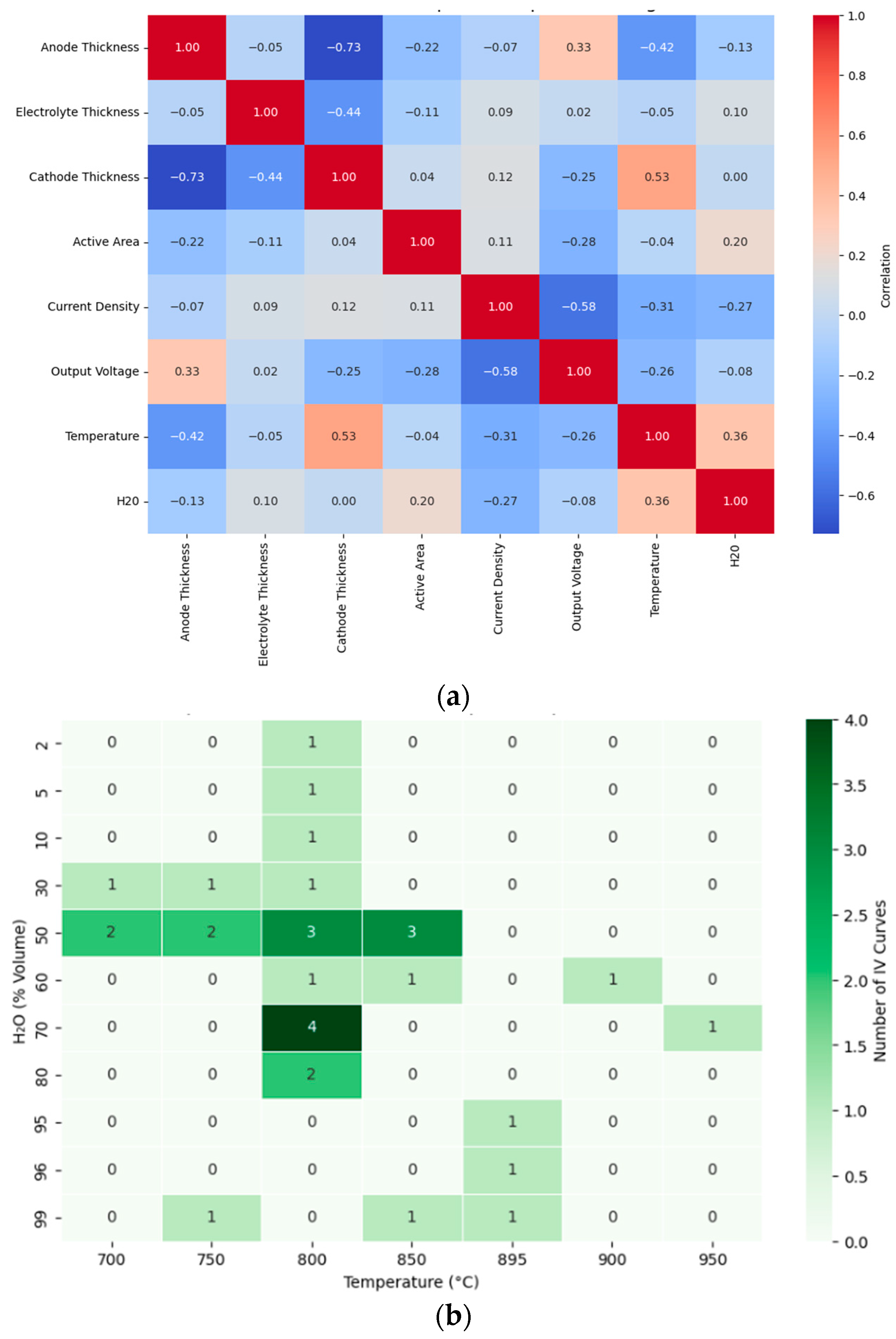
The correlation heatmap, Figure 2a, illustrates the relationship between various input features, anode thickness, electrolyte thickness, cathode thickness, active area, current density, temperature, and steam content (H2O%), and the output variable (output voltage) of solid oxide electrolysis cells (SOECs). From the correlation analysis, there is a strong negative (−0.73) correlation between cathode thickness and anode thickness, indicating that, as cathode thickness increases, anode thickness decreases significantly, and vice versa. This trend may be caused by the cell architecture (e.g., anode-supported vs. cathode-supported), where the thicknesses of the anode and cathode are usually inversely balanced. There is a moderate negative correlation (−0.58) between current density and output voltage, indicating that the output voltage decreases as current density increases. This behavior is consistent with the electrochemical behavior, where increased current density leads to higher ohmic losses and electrode overpotentials, resulting in voltage drops. Moreover, a moderate positive correlation (+0.53) was observed between temperature and cathode thickness. This suggests that, as cathode thickness increases, temperature also increases.
The heat map shown in Figure 2b was generated using the seaborn module on Python to show the distribution of the 31 IV curves collected from 12 articles based on their operating temperatures and gas composition (H2O%). From the heat map, it can be observed that most of the curves were measured at temperatures of 800 °C and 850 °C and at gas concentrations of 50% and 70% H2O composition.

3.3. Hyperparameter Tuning

Hyperparameter tuning was performed for each of the models used after training. This was achieved using Python programming via the scikit-learn library. The grid search method was used to produce the best parameters for the models [please see Supplementary Table S2 for the summary of the tuning methods and hyperparameter grid used per model]. A summary of the optimized parameters is shown in Table 2.

3.4. Cell Voltage Predictions

The performance of four (4) machine learning models, Random Forest (RF), Extreme Gradient Boost (XGBoost), Artificial Neural Network (ANN), and Support Vector Regression (SVR), was evaluated for predicting the output voltage of SOECs. The models were trained on 80% of the dataset and tested on the remaining 20%. Statistical metrics, coefficient of determination (R2), and Root Mean Squared Error (RMSE) were used to evaluate the predictive performance of the models and are summarized in Table 3. The XGBoost model demonstrated the highest performance, with 99.87% R2 for training and 98.39% R2 for testing. The RF model also achieved high performance, with 98.41% training R2 and 95.69% testing R2. However, there is a significant drop from training to testing, which indicates a low generalization capability of RF. On the other hand, the ANN model also achieved high performance with 98.70% training R2 and 97.72% testing R2, and, interestingly, it has the smallest performance gap between training and testing R2. This suggests the robust generalization capability of the model, which can capture the underlying relationships without overfitting. Lastly, the SVR model achieved the lowest performance with 93.17% training R2 and 91.02% testing R2. SVR’s low performance can be attributed to its inability to fully capture non-linear patterns.

3.5. Curve-Based Validation: Interpolation Tests

The performance of the four (4) models was then evaluated using a curve-based validation approach for predicting the IV curves of SOECs via interpolation and extrapolation tests. In the interpolation test, four complete IV curves were isolated as the test dataset to simulate the prediction of unseen combinations of operating conditions that are within the bounds of the input space. The models were also assessed using R2 and RMSE and are summarized in Table 4.
The Random Forest model achieved high training (98.86%) and testing R2 (98.34%) with low RMSE values, indicating the excellent generalizability of the model. The XGBoost model achieved a training R2 of 99.85% and testing R2 of 98.10% and achieved the lowest RMSE, indicating excellent generalization to unseen data, consistent with the cell voltage prediction results. The ANN model achieved a training R2 of 94.57% and testing R2 of 92.21%. The relatively low accuracy of ANN could be attributed to its limitations in handling relatively small datasets. Lastly, SVR achieved a training R2 of 92.85% and testing R2 of 97.11%, suggesting a good generalization to unseen data. Overall, RF and XGBoost emerged as the best-performing models for curve-based validation for the interpolation scenario, with XGBoost having the lowest RMSE.
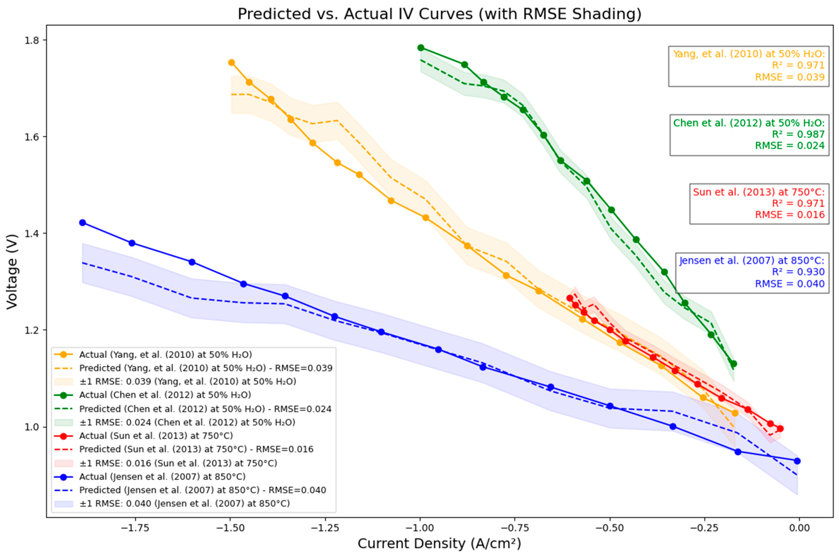
The resulting individual IV curve predictions of the interpolation tests are illustrated in Figure 3. For Chen et al. [29] and Yang et al. [35], unseen curves at 50% H2O gas composition were introduced. The model exhibited high predictive performance with an R2 value of 98.7% and 97.1%, respectively. This suggests a good generalizability of the model for predictions at 50% H2O, which is aligned with the findings for the heatmap distribution of the training data, where most of the collected IV curves have gas compositions set at 50%. For Sun et al. [36], an unseen curve at 750 °C was introduced and resulted in a high predictive performance of 97.1%. Although three (3) curves at 850 °C and 50% H2O were part of the collected data, as shown in Figure 2b, the prediction for Jensen et al. [12] still achieved a lower R2 of 93.0% compared to other curves. This may suggest that the curves collected were insufficient to fully represent the variability at this combination of operating conditions, possibly leading to less robust generalization.

3.6. Curve-Based Validation: Extrapolation Test

To test the predictive capability of the XGBoost model at extreme conditions, sample extrapolation tests were also conducted. Two (2) IV curve predictions were made for curves taken from Jensen et al. [12] with a cathode-supported cell at unseen high operating temperature of 950 °C and 70% H2O, and from Zhu et al. [34] with a cathode-supported cell at unseen and extremely low H2O% of 2% and operating temperature of 800 °C; these were isolated as test datasets for extrapolated curve-based validations.
Mahalanobis distance analysis (Table 5) indicated that neither case exceeded the 95% threshold, suggesting that the overall feature vectors fell within the multivariate distribution of the training dataset. However, the feature percentile ranks revealed that, for test case 1 (Jensen et al. [12] at 950 °C), temperature is part of the top 4% of all training values, while anode thickness and current density were near the minimum observed values. Additionally, for test case 2 (Zhu et al. [34]), H2O content and electrolyte thickness were at the absolute minimum, and current density is at the top 7% of the of the training values.
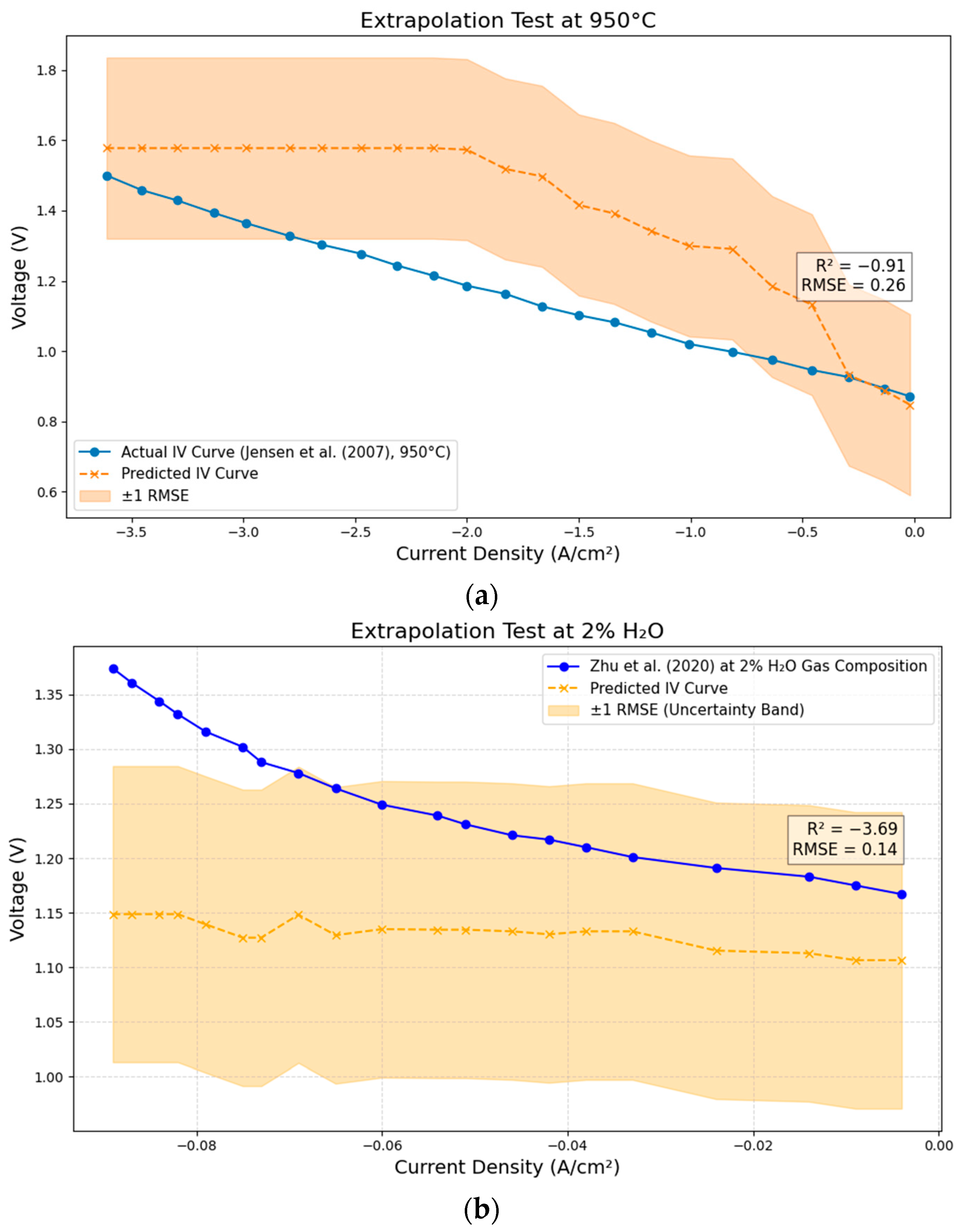
Using the XGBoost model, IV curves were plotted in Figure 4a,b. While the XGBoost model IV curve followed a decreasing trend for the cell voltage, it is highly evident that the shape of the predicted curve is far from the literature curve at 950 °C. This finding is also supported by the negative R2 of −0.0091%, where a negative R2 indicates that the predicted curve is performing worse than just a horizontal line prediction. Similar patterns are also observed with the prediction results at low H2O% of 2%, having an R2 of −369%, which suggests an even poorer prediction performance than that of the outlier temperature test. These results emphasize that, even with low Mahalanobis distances, models can still face risks if some features have extreme values. In such cases, performance drops may be driven by the single extreme values rather than their multivariate profile. The extrapolation findings expose a key limitation of data-driven models such as XGBoost when tested outside the training input distribution: machine learning can approximate relationships based on its learning from historical data, but it does not inherently understand or adapt to the underlying physical principles of material-specific behaviors. SOECs are strongly governed by material-specific properties such as conductivity, porosity, gas diffusivity, and activation energy, which are all highly sensitive to factors such as operating temperature, gas composition, and material configuration. The findings are in agreement with the existing literature that highlights extrapolation as a known weakness of machine learning. Moreover, the findings also emphasize the continued importance of materials science domain knowledge and experimental validation in SOEC advancement.

4. Conclusions

This study demonstrates the viability of machine learning (ML) as a predictive tool for modeling the electrochemical performance of solid oxide electrolysis cells (SOECs) with the material configuration LSM-YSZ/YSZ/Ni-YSZ under trained operating conditions. Four ML models, Support Vector Regressor (SVR), Random Forest (RF), Extreme Gradient Boosting (XGBoost), and Artificial Neural Network (ANN), were evaluated, with XGBoost showing the highest predictive performance. Specifically, XGBoost accurately predicted cell voltage and IV curves across varying gas compositions (50–70% H2O) and temperatures (700–800 °C), achieving R2 values of 98.39% and 98.10%, respectively, within the interpolation range. To explore the limits of model generalization, extrapolation cases were evaluated using Mahalanobis distances and percentile ranking per feature relative to the training dataset distribution. Findings revealed that, even when the overall multivariate distance is below the 95% threshold, certain single features, such as temperature and H2O%, were far beyond the training range, resulting in poor performance of the IV curve predictions. The findings highlight that, while ML models, like XGBoost, are effective at interpolation, they remain unreliable when faced with untrained, extreme conditions, where they cannot yet fully capture the underlying thermodynamic and microstructural factors influencing SOEC behavior. Moreover, this study emphasizes the critical importance of comprehensive and representative training data. Despite this, the high predictive accuracy within typical operating conditions confirms that machine learning, when applied with appropriate data coverage and guided by materials science concepts, can significantly accelerate SOEC design and optimization.

Supplementary Materials

The following supporting information can be downloaded at: https://www.mdpi.com/article/10.3390/app15179388/s1, containing the supporting charts and tables: Table S1: Summary of collected IV curves from 12 journal articles; Table S2: Summary of Evaluation Metrics for the machine learning models for the Cell Voltage Predictions compared by Imputation Method; Table S3: Hyperparameter Tuning Methods for the 4 models used for training; Figure S1: Actual vs Predicted Cell Voltage Values (top to bottom) (a) Random Forest Model, (b) XGBoost model, (c) ANN Model, (d) SVR Model; Figure S2–S13: IV Curve predictions of each article using XGBoost model.

Author Contributions

Conceptualization, N.G.A.E. and R.B.M.C.; methodology, R.B.M.C.; data collection/pre-processing/validation, N.G.A.E.; writing—original draft preparation, N.G.A.E.; writing—review and editing, R.B.M.C.; supervision, R.B.M.C. All authors have read and agreed to the published version of the manuscript.

Funding

This work is financially supported in part by the Department of Science and Technology—Engineering Research and Development for Technology (DOST-ERDT) MS Scholarship, the ERDT-Faculty Research Dissemination Grant (ERDT-FRDG), and the CHED-PCARI SureTech Project (Grant No. IIID-2018-009).

Data Availability Statement

Data supporting the findings of this study are available in the article and its Supplementary Materials. Additional data is available from the corresponding authors upon request.

Acknowledgments

The authors would like to acknowledge the financial support provided by the Department of Science and Technology Science Education Institute (DOST-SEI), by Engineering Research and Development for Technology (ERDT), and in part by the Philippine-California Advanced Research Institute—Commission on Higher Education (PCARI-CHED) through the Sustainable and Renewable Fuel and Electrolysis Cell Energy Device Technology (SureTech) research grant (IIID-2018-009). The authors are also grateful to Karla Ezra Pilario and Rogel Jan Butalid of the University of the Philippines Diliman for their valuable assistance and support.

Conflicts of Interest

The authors declare no conflicts of interest.

Abbreviations

The following abbreviations are used in this manuscript:
AIArtificial Intelligence
MLMachine Learning
SOECSolid Oxide Electrolysis Cell
SOFCSolid Oxide Fuel Cell
PEMPolymer Exchange Membrane
AEMAnion Exchange
IVCurrent–Voltage
ANNArtificial Neural Network
SVRSupport Vector Regressor
RFRandom Forest
XGBoostExtreme Gradient Boosting
IEAInternational Energy Agency
IRENAInternational Renewable Energy Association
CCSCarbon Capture and Storage
SMRSteam Methane Reforming
LSMLanthanum Strontium Manganite
YSZYttria-Stabilized Zirconia
Ni-YSZNickel Yttria-Stabilized Zirconia

References

  1. Herzog, A.; Tatsutani, M. A Hydrogen Future? An Economic and Environmental Assessment of Hydrogen Production Pathways. National Resources Defense Council (NDRC): New York, NY, USA, November 2005; Available online: https://www.nrdc.org/sites/default/files/hydrogen.pdf (accessed on 07 July 2025).
  2. International Energy Agency. IEA CO2 Emissions in 2023; International Energy Agency: Paris, France, 2023. [Google Scholar]
  3. IRENA. Making the Breakthrough: Green Hydrogen Policies and Technology Costs; International Renewable Energy Agency: Abu Dhabi, United Arab Emirates, 2021. [Google Scholar]
  4. Wolf, S.E.; Winterhalder, F.E.; Vibhu, V.; De Haart, L.G.J.; Guillon, O.; Eichel, R.-A.; Menzler, N.H. Solid Oxide Electrolysis Cells–Current Material Development and Industrial Application. J. Mater. Chem. A 2023, 11, 17977–18028. [Google Scholar] [CrossRef]
  5. Flis, G.; Wakim, G. Solid. Oxide Electrolysis: A Technology Status Assessment; Clean Air Task Force: Washington, DC, USA, 2023. [Google Scholar]
  6. Zong, S.; Zhao, X.; Jewell, L.L.; Zhang, Y.; Liu, X. Advances and Challenges with SOEC High Temperature Co-Electrolysis of CO2/H2O: Materials Development and Technological Design. Carbon. Capture Sci. Technol. 2024, 12, 100234. [Google Scholar] [CrossRef]
  7. Shirasangi, R.; Lakhanlal; Dasari, H.P.; Saidutta, M.B. Current-Voltage (i-V) Characteristics of Electrolyte-Supported (NiO-YSZ/NiO-SDC/ScSZ/LSCF-GDC/LSCF) Solid Oxide Electrolysis Cell during CO2/H2O Co-Electrolysis. Chem. Phys. Impact 2024, 9, 100670. [Google Scholar] [CrossRef]
  8. Stempien, J.P. Fundamental Aspects of Solid Oxide Electrolyzer Cell Modelling and the Application for the System Level Analysis. Ph.D. Thesis, Nanyang Technological University, Singapore, 2016. [Google Scholar]
  9. Kim, S.-D.; Seo, D.-W.; Dorai, A.K.; Woo, S.-K. The Effect of Gas Compositions on the Performance and Durability of Solid Oxide Electrolysis Cells. Int. J. Hydrogen Energy 2013, 38, 6569–6576. [Google Scholar] [CrossRef]
  10. Kupecki, J.; Niemczyk, A.; Jagielski, S.; Kluczowski, R.; Kosiorek, M.; Machaj, K. Boosting Solid Oxide Electrolyzer Performance by Fine Tuning the Microstructure of Electrodes–Preliminary Stud. Int. J. Hydrogen Energy 2023, 48, 26436–26445. [Google Scholar] [CrossRef]
  11. Shiva Kumar, S.; Lim, H. An Overview of Water Electrolysis Technologies for Green Hydrogen Production. Energy Rep. 2022, 8, 13793–13813. [Google Scholar] [CrossRef]
  12. Jensen, S.H.; Larsen, P.H.; Mogensen, M. Hydrogen and Synthetic Fuel Production from Renewable Energy Sources. Int. J. Hydrogen Energy 2007, 32, 3253–3257. [Google Scholar] [CrossRef]
  13. Liang, M.; Yu, B.; Wen, M.; Chen, J.; Xu, J.; Zhai, Y. Preparation of LSM–YSZ Composite Powder for Anode of Solid Oxide Electrolysis Cell and Its Activation Mechanism. J. Power Sources 2009, 190, 341–345. [Google Scholar] [CrossRef]
  14. Nechache, A.; Hody, S. Alternative and Innovative Solid Oxide Electrolysis Cell Materials: A Short Review. Renew. Sustain. Energy Rev. 2021, 149, 111322. [Google Scholar] [CrossRef]
  15. Grondin, D.; Desuere, J.; Brisse, A.; Zahid, M. Ozil Multiphysics Modeling and Simulation of a Solid Oxide Electrolysis Cell. In Proceedings of the COMSOL Conference, Hannover, Germany, 4–6 November 2008. [Google Scholar]
  16. Mendoza, R.M.; Mora, J.M.; Cervera, R.B.; Chuang, P.-Y.A. Experimental and Analytical Study of an Anode-Supported Solid Oxide Electrolysis Cell. Chem. Eng. Technol. 2020, 43, 2350–2358. [Google Scholar] [CrossRef]
  17. Menon, V.; Janardhanan, V.M.; Deutschmann, O. A Mathematical Model to Analyze Solid Oxide Electrolyzer Cells (SOECs) for Hydrogen Production. Chem. Eng. Sci. 2014, 110, 83–93. [Google Scholar] [CrossRef]
  18. Lee, J.H.; Shin, J.; Realff, M.J. Machine Learning: Overview of the Recent Progresses and Implications for the Process Systems Engineering Field. Comput. Chem. Eng. 2018, 114, 111–121. [Google Scholar] [CrossRef]
  19. Dobbelaere, M.R.; Plehiers, P.P.; Van De Vijver, R.; Stevens, C.V.; Van Geem, K.M. Machine Learning in Chemical Engineering: Strengths, Weaknesses, Opportunities, and Threats. Engineering 2021, 7, 1201–1211. [Google Scholar] [CrossRef]
  20. Jain, A. Machine Learning in Materials Research: Developments over the Last Decade and Challenges for the Future. Curr. Opin. Solid. State Mater. Sci. 2024, 33, 101189. [Google Scholar] [CrossRef]
  21. Allal, Z.; Noura, H.N.; Salman, O.; Chahine, K. Machine Learning Solutions for Renewable Energy Systems: Applications, Challenges, Limitations, and Future Directions. J. Environ. Manag. 2024, 354, 120392. [Google Scholar] [CrossRef] [PubMed]
  22. Langner, E.; Dehghani, H.; Hachemi, M.E.; Belouettar–Mathis, E.; Makradi, A.; Wallmersperger, T.; Gouttebroze, S.; Preisig, H.; Andersen, C.W.; Shao, Q.; et al. Physics-Based and Data-Driven Modelling and Simulation of Solid Oxide Fuel Cells. Int. J. Hydrogen Energy 2024, 96, 962–983. [Google Scholar] [CrossRef]
  23. Shomope, I.; Al-Othman, A.; Tawalbeh, M.; Alshraideh, H.; Almomani, F. Machine Learning in PEM Water Electrolysis: A Study of Hydrogen Production and Operating Parameters. Comput. Chem. Eng. 2024, 194, 108954. [Google Scholar] [CrossRef]
  24. Yang, Q.; Zhao, L.; Xiao, J.; Wen, R.; Zhang, F.; Zhang, D. Machine Learning-Assisted Prediction and Optimization of Solid Oxide Electrolysis Cell for Green Hydrogen Production. Green. Chem. Eng. 2024, 6, 154–158. [Google Scholar] [CrossRef]
  25. Zhang, C.; Liu, Q.; Wu, Q.; Zheng, Y.; Zhou, J.; Tu, Z.; Chan, S.H. Modelling of Solid Oxide Electrolyser Cell Using Extreme Learning Machine. Electrochim. Acta 2017, 251, 137–144. [Google Scholar] [CrossRef]
  26. Fei, Y.; Li, A.; Zhang, C.; Tu, H.; Zhu, L.; Huang, Z. Performance Optimization of Solid Oxide Electrolysis Cell for Syngas Production by High Temperature Co-Electrolysis via Differential Evolution Algorithm with Practical Constraints. Energy Convers. Manag. 2024, 300, 117911. [Google Scholar] [CrossRef]
  27. Zhao, Z.; Wang, X.; Tang, S.; Cheng, M.; Shao, Z. High-Performance Oxygen Electrode Ce0.9Co0.1O2-δ-LSM-YSZ for Hydrogen Production by Solid Oxide Electrolysis Cells. Int. J. Hydrogen Energy 2021, 46, 25332–25340. [Google Scholar] [CrossRef]
  28. Ebbesen, S.D.; Mogensen, M. Electrolysis of Carbon Dioxide in Solid Oxide Electrolysis Cells. J. Power Sources 2009, 193, 349–358. [Google Scholar] [CrossRef]
  29. Chen, Y.; Bunch, J.; Jin, C.; Yang, C.; Chen, F. Performance Enhancement of Ni-YSZ Electrode by Impregnation of Mo0.1Ce0.9O2+δ. J. Power Sources 2012, 204, 40–45. [Google Scholar] [CrossRef]
  30. Laguna-Bercero, M.A.; Campana, R.; Larrea, A.; Kilner, J.A.; Orera, V.M. Steam Electrolysis Using a Microtubular Solid Oxide Fuel Cell. J. Electrochem. Soc. 2010, 157, B852. [Google Scholar] [CrossRef]
  31. Kim-Lohsoontorn, P.; Bae, J. Electrochemical Performance of Solid Oxide Electrolysis Cell Electrodes under High-Temperature Coelectrolysis of Steam and Carbon Dioxide. J. Power Sources 2011, 196, 7161–7168. [Google Scholar] [CrossRef]
  32. Li, Q.; Kuang, K.; Sun, Y.; Zheng, Y.; Liu, Q.; Chan, S.H.; Zhang, H.; Wang, W.; Li, T.; Wang, J. Deficiency of Hydrogen Production in Commercialized Planar Ni-YSZ/YSZ/LSM-YSZ Steam Electrolysis Cells. Int. J. Hydrogen Energy 2022, 47, 23514–23519. [Google Scholar] [CrossRef]
  33. Hauch, A.; Jensen, S.H.; Ramousse, S.; Mogensen, M. Performance and Durability of Solid Oxide Electrolysis Cells. J. Electrochem. Soc. 2006, 153, A1741. [Google Scholar] [CrossRef]
  34. Zhu, Z.; Sugimoto, M.; Pal, U.; Gopalan, S.; Basu, S. Electrochemical Cleaning: An in-Situ Method to Reverse Chromium Poisoning in Solid Oxide Fuel Cell Cathodes. J. Power Sources 2020, 471, 228474. [Google Scholar] [CrossRef]
  35. Yang, C.; Jin, C.; Coffin, A.; Chen, F. Characterization of Infiltrated (La0.75Sr0.25)0.95MnO3 as Oxygen Electrode for Solid Oxide Electrolysis Cells. Int. J. Hydrogen Energy 2010, 35, 5187–5193. [Google Scholar] [CrossRef]
  36. Sun, X.; Chen, M.; Liu, Y.-L.; Hjalmarsson, P.; Ebbesen, S.D.; Jensen, S.H.; Mogensen, M.B.; Hendriksen, P.V. Durability of Solid Oxide Electrolysis Cells for Syngas Production. J. Electrochem. Soc. 2013, 160, F1074–F1080. [Google Scholar] [CrossRef]
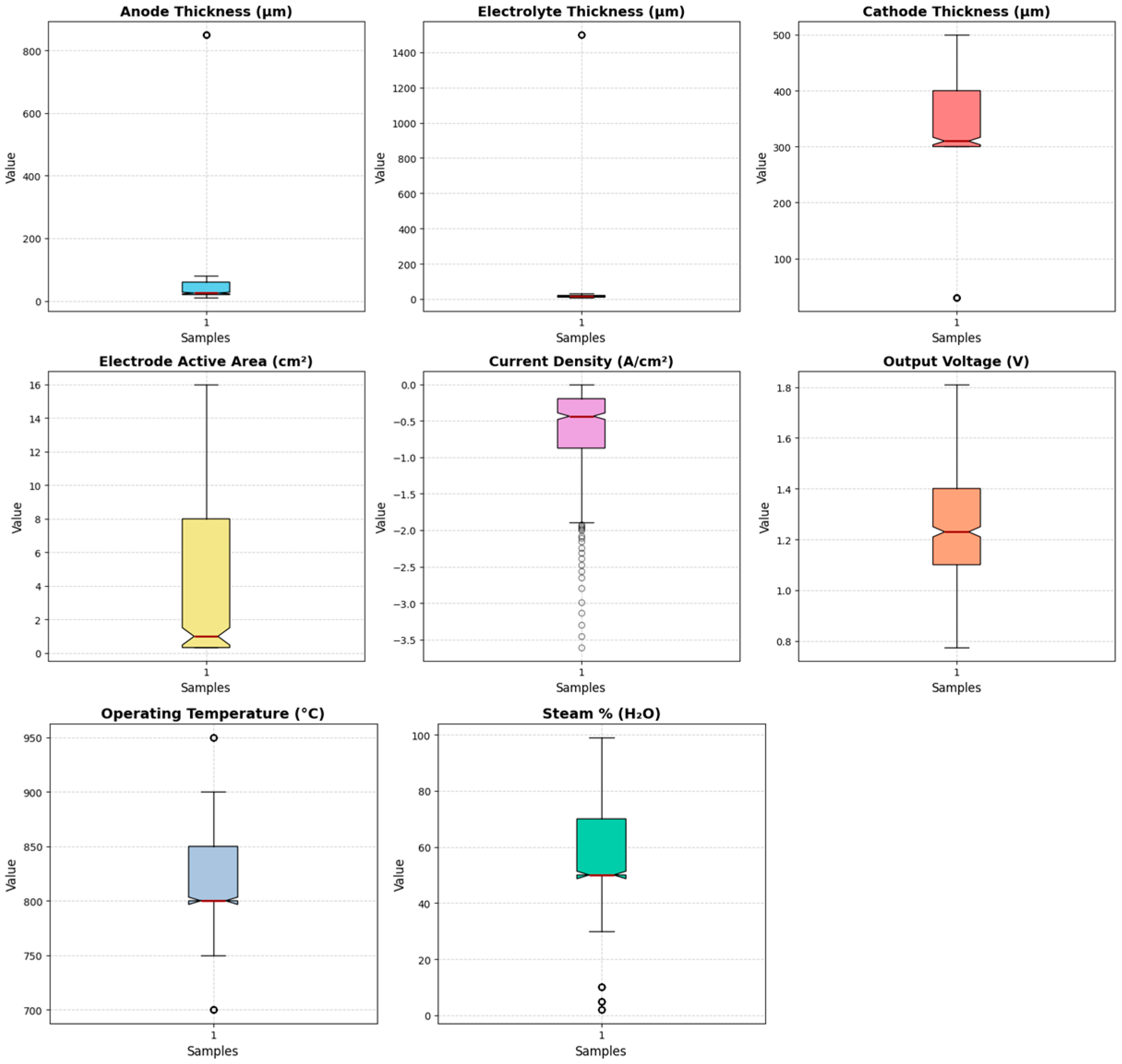
Figure 1. Distribution analysis for the input and output variables.
Applsci 15 09388 g001
Figure 2. (a) Correlation analysis of the input and output variables. (b) Distribution heatmap of the unique IV curves collected plotted against H2O% and operating temperatures.
Applsci 15 09388 g002
Figure 3. IV curve interpolation tests using unseen curves that have operating conditions within the bounds of the input space [12,29,35,36].
Applsci 15 09388 g003
Figure 4. (a) IV curve extrapolation test using Jensen et al. [12] at 950 °C operating temperature and (b) IV curve extrapolation test using Zhu et al. [34] at 2% H2O gas composition.
Applsci 15 09388 g004
Table 1. Data profiling results of the collected features.
Feature CategoryFeatureRangeUnit/s%Missing
Cell CharacteristicsAnode Thickness10–850µm8.43%
Cathode Thickness30–500µm8.43%
Electrolyte Thickness7–1500µm8.43%
Active Area0.33–63cm20%
Operating ParametersTemperature700–950°C0%
Gas Composition (H2O%)2–99%%0%
Electrolytic ParametersCurrent Density−3.611 to −0.002A/cm20%
Cell Voltage0.774–1.810Volts0%
Table 2. Optimized hyperparameters for all the ML algorithms.
ModelHyperparametersOptimized Parameters
Random Forest (RF)N Estimators200
Max Depth16
Min Samples Split2
Min Samples Leaf2
XGBoostN Estimators500
Max Depth3
Learning Rate0.2
Subsample0.8
Colsample by Tree1.0
ANNNo. of Hidden Layers2
Hidden Layer Size64
ActivationReLU
OptimizerAdam (default learning rate = 0.001)
Epochs100 (early stopped)
Batch Size32
Early StoppingYes, patience = 10
SVRC1
KernelRbf
GammaScale
Epsilon0.01
Table 3. Summary of evaluation metrics for the machine learning models for the cell voltage predictions.
ModelEvaluation MetricResults
Random Forest (RF)Training R298.41%
Training RMSE0.0270
Testing R295.69%
Testing RMSE0.0448
XGBoostTraining R299.87%
Training RMSE0.0077
Testing R298.39%
Testing RMSE0.0274
ANNTraining R298.70%
Training RMSE0.0244
Testing R297.72%
Testing RMSE0.0326
SVRTraining R293.17%
Training RMSE0.0059
Testing R291.02%
Testing RMSE0.0647
Table 4. Summary of evaluation metrics of the ML models for the curve-based validation for the interpolation scenario.
ModelEvaluation MetricResults
Random Forest (RF)Training R298.86%
Training RMSE0.0223
Testing R298.34%
Testing RMSE0.0598
XGBoostTraining R299.85%
Training RMSE0.0081
Testing R298.10%
Testing RMSE0.0332
ANNTraining R294.57%
Training RMSE0.0488
Testing R292.21%
Testing RMSE0.0673
SVRTraining R292.85%
Training RMSE0.0559
Testing R297.11%
Testing RMSE0.0647
Table 5. Mahalanobis distance analysis and feature percentile ranks of the extrapolation test cases [12,34].
Test CaseMahalanobis
Distance
95%
Threshold
99%
Threshold
Multivariate
Outlier?
Feature
Percentile Ranks 1
1
(Jensen et al. [12])
3.31384.30885.1154NoAnode thickness: 0%
Electrolyte thickness: 12.31%
Cathode thickness: 36.93%
Active area: 63.24%
Current density: 4.05%
Temperature: 96.12%
H2O%: 59.70%
2
(Zhu et al. [34])
2.24664.30885.1154NoAnode thickness: 39.63%
Electrolyte thickness: 0%
Cathode thickness: 80.10%
Active area: 50.93%
Current density: 93.42%
Temperature: 18.38%
H2O%: 0%
1 Percentile ranks were calculated relative to the training dataset.
Disclaimer/Publisher’s Note: The statements, opinions and data contained in all publications are solely those of the individual author(s) and contributor(s) and not of MDPI and/or the editor(s). MDPI and/or the editor(s) disclaim responsibility for any injury to people or property resulting from any ideas, methods, instructions or products referred to in the content.