Abstract
Predictive maintenance of railroads is essential to prevent costly disruptions. A critical aspect of this maintenance is ensuring the integrity of the pantograph-catenary system, where copper alloy wires experience continuous friction and wear. The degradation rate and condition of these wires are vital factors in planning maintenance activities. Current wear rate prediction methods are largely theoretical and often inaccurate, overlooking essential contextual details. Additionally, wire condition data frequently show inaccuracies and inconsistencies in spatial and temporal resolution, complicating the feasibility of using data-driven approaches. This research investigates a data-driven framework to accurately predict wear rates, emphasizing data processing and optimized data use. A dataset spanning nine years of Dutch railway infrastructure measurements is used, employing various machine learning techniques to determine the most effective approach. Findings indicate that, in 95% of cases, average wire thickness can be predicted with a precision of ±0.12 mm over a four-year period. This study advances the field by proposing a framework that addresses measurement errors, a common challenge in sensor-based assessments, making data-driven maintenance a more reliable option.
1. Introduction
Railway transportation has become a vital component of modern society, on which the smooth functioning of many aspects of modern life depends [1,2]. The high dependency on this mode of transportation means that the maintenance and upkeep of the railroad infrastructure are of cardinal importance [3,4]. Given that the railroad is a high-maintenance asset, the maintenance expenditure can be a significant part of the overall lifecycle costs [4,5,6,7]. Therefore, even small improvements in mainstream maintenance practices can potentially amount to significant savings. Schedule-based and periodic maintenance of railroads (i.e., preventive maintenance) can be costly because it requires resources to be allocated to all parts of the railroad, equally and irrespective of how different parts of the asset may or may not need more immediate attention [8]. That is why predictive maintenance, which focuses on predicting the condition of the asset based on actual inspection data and applying maintenance based on the predicted condition, is becoming a more preferred approach for modern railroad management [9,10]. Inspection, continuous monitoring of the asset condition, and the prediction of the future condition are the backbone of preventive maintenance. There are a wide range of solutions for the inspection and condition assessment of railways [2,11,12,13,14,15]. For instance, Wang et al. [12] developed a CNN-LSTM model to predict the geometric deformation of railway tracks.
The catenary system is an integral part of electric trains, as shown in Figure 1. This system comprises many parts, including fasteners, droppers and contact wires. Maintenance of the catenary system involves the upkeep of all these components. Several research works have focused on modelling the degradation mechanism and maintenance of these parts. For instance, Wu et al. [16] and Meng et al. [17] proposed different methods for fault detection of fasteners. One component of the railway, which is critical for the functionality of electric trains, is the contact wire. As shown in Figure 1, contact wires are a part of the overhead power line that transports the electricity parallel to the track. A train makes contact with the copper contact wire through a pantograph, which allows it to draw electricity. To make proper contact with the contact wire, the pantograph exerts a force upwards pressing against the wire. When the train moves, this will induce friction and eventually wear down the pantograph and contact wire. Over time, the contact wire decreases in size to the point where it must be replaced.
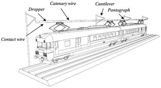
Figure 1.
Schematic representation of catenary system of electrified railways.
With the ongoing increase in train traffic, it is expected that the average lifespan of contact wires will decrease. Asset owners are striving to transition to predictive maintenance [18,19,20]. This shift enables maintenance activities to be strategically planned based on the prediction of asset conditions. Predictive maintenance allows for different maintenance activities to be combined when they concern the same section. This will reduce downtime and increase the reliability of transportation schedules. Accurately predicted asset conditions allow for a more optimal replacement strategy [21].
The current predictive maintenance methods for contact wires use numerical models to predict different failure modes such as tension, fatigue, and wear [22,23,24,25,26,27]. These models try to capture the wear mechanism of the contact wire in physics-based models and use it for the prediction of the remaining life. While these methods have a strong theoretical basis and are shown to be accurate under some conditions, they assume a certain degree of determinism and stability in the circumstances surrounding the wear mechanism, which reduces the generalizability and accuracy of the models. For instance, parallel wires may wear at different rates because they are not exactly at the same height. This misalignment causes one wire to sustain more friction and thus wear at a different rate. While the mechanics behind this are not too difficult to model, many of the existing models ignore these scenarios to reduce the computational intensity of their models. This has a negative impact on the accuracy of the models and, therefore, their reliability.
The wear mechanism of contact wires is governed by a myriad of factors and is complex. The most important factor is the number of train passages, which directly influences the rate at which the wire loses its volume due to friction [28,29]. The electrical current is also often mentioned as being a significant contributor as this causes the wire to heat up and experience mechanical stress [30]. The electrical current is the highest during acceleration and deceleration which makes these zones more prone to wear [26]. The contact force is another factor influencing the wear. If the contact force is too low the pantograph will vibrate, bounce and create electrical arcs. If the contact force is too high, it will result in excessive friction [31]. Another wear factor that is often mentioned in the literature is the train’s speed. More heat will be generated at higher speeds which is partly caused by the higher electrical current. Shing [29] found that the wear rate increases when the relative speed is higher. All these parameters need to be taken into account to ensure high accuracy of the wear rate prediction.
Nowadays, asset owners collect a wide array of valuable data about the train passages and many other parameters (e.g., age, current thickness, applied force, etc.) about the train track [20]. This data could be used to develop data-driven models that capture many wear scenarios and mechanisms [32,33,34]. Several research studies have indicated how asset condition data can be leveraged to establish data-driven models for predictive maintenance [35,36,37,38,39,40]. For instance, Xu et al. [41] have shown that a data-driven condition assessment model can be developed even with a small set of annotated data. In these models, Machine Learning (ML) methods correlate diverse influential parameters with the wear/degradation mechanism based on historical data [42]. With the advent of sensory data and normalization of systematic data collection routines, railway asset managers nowadays have built up substantial databases that allow them to use more sophisticated deep learning-based models for predictive maintenance [43,44,45]. A recent research trend focused on the use of data-driven modelling for the condition assessment of catenary systems [46,47,48,49,50,51,52,53]. It is indicated that ML-based predictive maintenance is one of the top priorities in the railway sector [20,54]. Given the complexity of the catenary system, predictions can be made about the condition of different aspects. For example, Gregori et al. [47] tried to predict the contact force as an indication of the condition of the entire system. Kuznar and Lorenc [48] focused on the wear of sliding strips and successfully used ML to predict the condition of this component. Yang et al. [51] deployed a Convolutional Neural Network to detect defective droppers in the catenary system. Huang et al. [46] developed surrogate models for the assessment of the catenary system quality, evaluated in terms of energy transfer quality. However, they focused on the entire system rather than contact wires specifically. While useful, these models are not very practical for making decisions on the maintenance of wires since they do not indicate the root causes of the deteriorating quality. Additionally, they used physics-based models to generate data for the surrogate modelling. The main limitation of this approach is that since the baseline data is simulated, they inherit the intrinsic inaccuracies of the simulation models. Blanco et al. [49] used simulated data and machine learning to predict the excessive lateral displacement of the contact wire due to a faulty steady arm. While these methods are useful, from the maintenance perspective they have less relevance because the intervention strategies (replacement, repair, etc.) need to focus on specific components. Given that contact wires are one of the most significant components of the catenary system and also given that their maintenance is costly, it is imperative to be able to monitor their condition independently of the entire catenary system. To the best of the authors’ knowledge, data-driven modelling of contact wire wear is largely understudied. In a rare instance, Moussallik [55] tried to develop a condition assessment framework for contact wires using a computer vision approach. Yet again, the proposed approach is limited to the vision-based condition assessment of wires and does not focus on the prediction of their wear. Finally, Usuda [28] used Neural Network to estimate the wear rate and strain of contact wires and achieved good accuracy. However, in the absence of actual measurement data, he resorted to simulated data for the training and testing of the model. The main limitation of this approach is that the simulated data commonly do not completely represent the natural fluctuations in the data, given that they are generated based on the limited view of complex wear physics.
To this end, this paper aims to develop and investigate the feasibility of data-driven models for the prediction of the contact wire wear rate based on a wide range of affecting factors and using time-series measurement data. The data used in this study were collected by measurement trains from the Dutch railway system, which measure the wire thickness roughly once every year. The dataset contains measurements that span from 2010 to 2018. A data-driven pipeline for the wear rate of wire is an intricate process, given the multi-dimensional nature of the problem and the inherent inaccuracies of the current data collection and measurement techniques and instrumentation. Therefore, it is very critical to holistically analyze the available data and develop a data processing mechanism that can ensure accurate modelling of the wear rate. The proposed data processing mechanism is built solely on the assumption of the availability of wire thickness measurement. Therefore, it is expected to be generalizable to other railway systems where similar measurements are carried out as part of the routine asset management practices. Hence, this research offers insight into a robust framework for the preparation and processing of the raw measurement data for the successful application of data-driven modelling.
2. Research Methodology
Figure 2 presents the overview of the research methodology applied in this research. In general, the research comprises four phases: data collection, data preparation, model development, and performance assessment. Some of these phases consist of several steps. The remainder of this section discusses each of these phases in more detail.
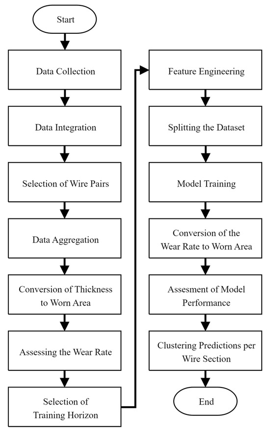
Figure 2.
Overview of the research methodology.
2.1. Data Collection
Table 1 presents the most important factors that affect the wear rate of contact wires. These factors are derived from the study of relevant literature presented in Section 1. The necessary information for the quantification of these factors is extracted from the databases of ProRail, which is responsible for the maintenance of the national railway in the Netherlands. These datasets contain: (1) data collected by measurement trains, (2) train traffic data, and (3) train speed data. The measurement train measures the properties of the contact wires roughly every year for all tracks in the Netherlands. Besides the thickness of the contact wire, the train measures other parameters such as pantograph contact force, horizontal wire position, wire height, and cant. The dataset contains measurements from 2010 to 2018. These measurements are combined in one dataset with details about their location. At 45 locations in the Netherlands, the deflection of the rail is measured and collected in a database called Quo Vadis. From the rail deflection, the load per axis is derived. This combined with information about the train formation and its scheduled route can help calculate the number of passed trains and the total weight for every rail section. This information is available per month for passenger and freight trains. The location and the speed of every train are registered by the control centre. This information is collected for a single day when the average speed is calculated for segments of 100 m for all train passages. It is assumed that the average train speed on this day is representative of the average railroad traffic throughout the year.

Table 1.
Features used for the prediction of wear rate.
In general, the features used in the model can be divided into seven categories:
- (1)
- Contact wire properties: The measurement train has two measurements for each wire; the average and minimum values are measured over 25 cm. For both measurements, a feature is created by taking the average and minimum values for all measurements in the 10 m block. Also, the standard deviation is derived from these measurements. This feature indicates the roughness of the wire within the block of 10 m. Another feature based on the contact wire is the delta thickness. This is the difference in thickness between the left and the right wire. This delta thickness is calculated for the average and minimum measured thickness.
- (2)
- Position wire: The measurement train measures the position of the wire in relation to the centre of the track. The height is one feature that is created based on the vertical position of the wire. The height is measured for both wires which allows the creation of a feature that indicates the delta height between the two wires. Also, the horizontal position is measured, which generates a feature that indicates the distance between the wire and the centre of the track.
- (3)
- Cant: The cant of the track is measured by the measurement train. The tilt of the track indicates indirectly if the 10 m block is located in a curved section of the track. This is because cant is applied to compensate for the centrifugal forces during a turn.
- (4)
- Speed: The measurement train logs its speed while measuring. This speed is used as a feature to indicate the relative speed of trains. Each section of a track has also a maximum allowed speed. This is used as another feature as trains often try to approach this maximum speed. A third feature to estimate the train speed is based on the average speed of trains logged per 100 m. This logged data is based on recordings of only one day but is likely the best estimate for the actual train speed. Based on this data, the difference in speed is also calculated. This feature indicates the acceleration and deceleration which indirectly estimate the electrical current.
- (5)
- Passed trains: Between the most important railroad switches, the number of passed trains is measured. For this, a distinction is made between trains transporting passengers and goods which are both used as a feature. Also, the total number of passed trains is a feature. The number of trains is an indicator of the number of passed pantographs that have been in contact with the contact wire. This feature can be adjusted if more or fewer trains will pass in the future.
- (6)
- Transported tons: The number of tons is measured in the same way as the number of passed trains. The number of tons is known for trains transporting passengers, goods and both combined. For all three measurements, a feature is created. The number of tons transported can be used as an indirect estimate for the total electrical load exerted on the contact wire.
- (7)
- Historical trend: Based on the data points used for the input of the model, a wear rate trend can be created for this specific period. With linear regression, a trend line can be calculated based on the worn area for the selected data points. The historical trend is used as a feature which is an indication of the expected wear rate for an extended time. Increasing the number of used data points will improve the stability and accuracy of the slope. The R2 score of the regression line is also used as a feature to indicate the reliability of the slope. This feature must not be confused with the label of the model. Both apply the same principle; however, this feature only uses the data points of the input horizon instead of all data points.
2.2. Data Integration
To link the three datasets, the section ID and kilometrage of the tracks are used to create a unique ID. In case data is missing in one of the datasets, the associated ID is excluded from the study. Also, IDs with less than 8 data points per ID are removed. To make the model more robust, unique cases (i.e., outliers) are removed. For instance, almost all contact wires in the Netherlands have an initial diameter of 12 mm. Only a few segments are using wires with a diameter of 13 mm. These segments are excluded from this study. Also, tracks which are used for high-speed rail are excluded, as these tracks have different overhead wire specifications.
2.3. Selection of Wire Pairs
Above a single train track, there are two contact wires which form a pair. During the transition between wire sections, there are two overlapping pairs of wires. One wire pair slowly increases in height while the new wire pair slowly decreases its height, as shown in Figure 3.
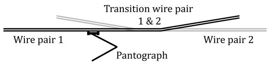
Figure 3.
Side view of transition between wire pairs.
During this transition, the measurement train measures the pairs simultaneously. However, it does not indicate which wire is in contact with the pantograph. Because the lowest wire is more likely to be in contact with the pantograph, it is assumed that the two lowest wires are in contact with the pantograph. If the difference in height between two wires is found to be more than 3 mm, the data point is removed as this seemed not realistic. Because contact wires are replaced in pairs, the measured parameters of the two wires are combined into one. Thus, each wire pair is presented by an average and minimal value of the pair. The average and minimum thickness are both used as a feature, together with the delta thickness between the two wires.
2.4. Data Aggregation
As mentioned above, the measurement train performs a measurement every 25 cm along the contact wire. One problem with this data is that the accuracy of the measurements is low due to deviations in the registered location and the precision of the thickness measurement itself. To reduce the noise of these measurements and to reduce the computation time, data points are aggregated for every 10 m of measurements. This means that if all data points are valid, each data point aggregates 40 raw measurements. The way these 40 data points are aggregated varies per feature. For most features, the average of the values is used. But other transformations such as the minimum and the standard deviation are used. Table 1 presents the applied transformation for every feature.
2.5. Conversion of Thickness to Area
Due to the round shape of the wire, the decrease in thickness is not linear. In the new condition, the contact wire has a small contact area. This means that the wire thickness will decrease faster when it is new. If the wire wears down, the contact area will increase which results in a slower wear rate for thickness. An example of this phenomenon is shown in Figure 4. With a wire of 12 mm in diameter, the first worn millimetre is equivalent to 4.5 mm2. However, when the remaining thickness is 8 mm, 11.6 mm2 needs to be removed for the thickness to decrease by another millimetre.
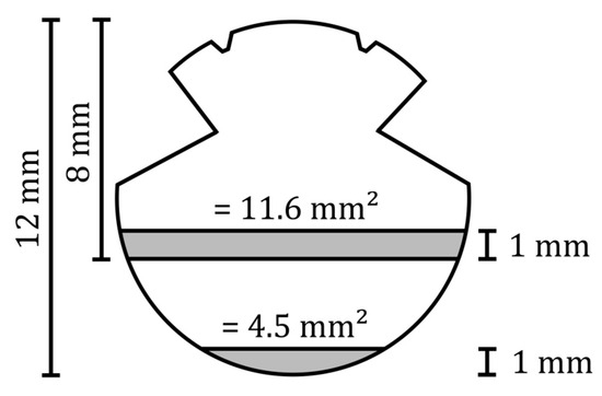
Figure 4.
Schematic representation of the relationship between wire thickness and wire surface.
According to Archard [56], the removed material due to wear is proportional to the work applied by friction forces. This means that with the same frictional force, a fixed volume of debris will be removed. As can be seen in Equation (1), the contact area is not relevant for the worn volume.
where
In the case of contact wires, the frictional force will be the pantograph that slides along the wire. The occurring wear in relation to the passed pantographs will be linear in terms of volume according to Archard [56]. If possible, linear relations are preferred when analyzing data. Therefore, the thickness is translated into a volumetric degradation. This is accomplished by using Equation (2). This equation gives the worn area based on the radius and thickness of the wire. In Figure 5, the variables of the formula are visualized whereby the worn area is shown in grey.
where
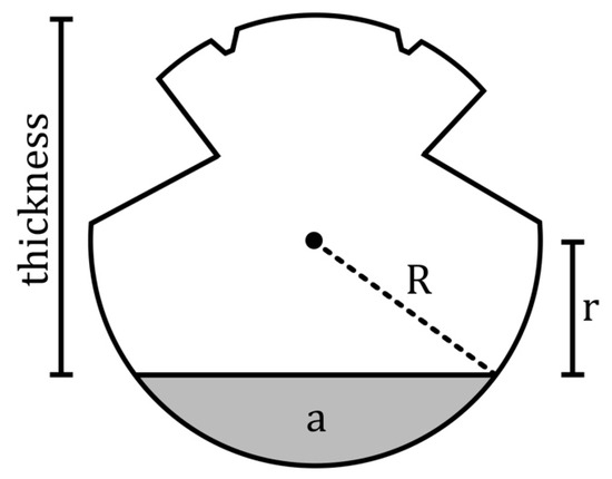
Figure 5.
Conversion of wire thickness to worn area.
2.6. Assessing the Wear Rate
The fundamental principle of the wear rate prediction model is to determine the potential wear rate of the wire based on given feature values. To train the model, a wear rate is needed which can be linked to the features. This wear rate is the desired output of the model and is called the ‘label’. The wear rate is expressed in square millimetres of copper that wears down per year (mm2/year).
Since the measurement data is noisy, it is impossible to know the exact yearly wear rate. Therefore, an approximation is made based on historical data. As train schedules and other factors are rather constant for each year, no disrupting changes are expected for the wear rate. The wear rate label is determined using linear regression for all years for which data is available. By doing this, the data of all years are utilized to estimate a reliable wear rate that is constant for the whole period. In schematic Figure 6, it can be seen that the data from multiple years is transformed into a single yearly wear rate.
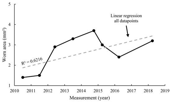
Figure 6.
Generation of wear rate label by linear regression over all data points.
In some cases, the deviations in the data are too large to fit a reliable wear rate. These cases could be detected by looking at the R2 score which is given for the fitted regression line. If the R2 score is low, the regression line does not represent the data well, which is in most cases caused by extreme noise. The slope of the fitted regression line is a second indicator to detect unreliable results. A line could be fitted with a slope that suggests a negative wear rate. This is physically impossible as the worn area can only increase. One possible scenario for such cases is a replacement of the wire. Wire replacements are not registered in a structured way and can thus only be detected properly by analyzing the data throughout the years. Another reason for an unreliable wear rate is the number of available data points. The more data points, the higher the reliability of the wear rate generated by linear regression. For reliable wear rates, the data must thus be filtered on reasonable R2 scores, positive slopes and the minimum number of available data points. For this research, R2 scores below 0.4 are removed. The same is applied for negative wear rates and locations with less than 8 data points.
2.7. Selection of Training Horizon
As mentioned above, the model tries to associate features with a measured wear rate. Given that the wear rate is determined based on the regression of all measurements, the measurement data need to be aggregated into a single data point that represents a set of features. It is important to use only a few data points for this aggregation. This is because fewer points can better capture the extent to which features influence the prediction of wear rate. This is especially desired in cases where the state of the asset may change suddenly. The more data points are used for the training horizon, the more flattened the output will be. Especially if the data contains a lot of noise, smoothing is necessary to avoid outliers influencing the output too much. However, the downside of including many data points for training is that fine details in the relationship between features and the wear rate could become diluted. With noisy signals, it is hard to determine if an outlier is a change in asset condition or just noise. Therefore, an optimum has to be found between the stability and responsiveness of the model, as will be explained in Section 2.12.
The portion of data used for training is called the training horizon in this research. In other words, the training horizon determines how many of the data points are included for training. The individual data points within the training horizon are combined into a grouped data point per feature. For this, the average of each feature is calculated for all included data points. The period of the training horizon is selected randomly. In the example of Figure 7, this period ranges from 2013 to 2016. Randomly shifting the training horizon over time avoids biases induced by trends in the data. Also, measurement offsets for specific years are neutralized by this method.
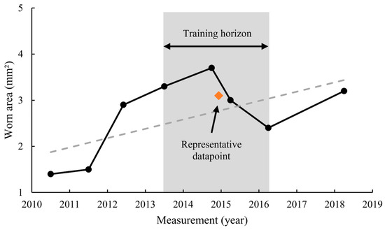
Figure 7.
Random selection of training horizon.
2.8. Feature Engineering
Figure 8 presents the feature engineering that is undertaken at this point. As mentioned before, the data in the training horizon needs to be aggregated. But as explained in Section 2.4, each data point is already the result of aggregating raw measurements over a length of 10 m. In the next step, the spatially aggregated data need to be re-aggregated temporally so that one set of features would represent the training horizon. The features from multiple dates are combined by taking the average of all dates. At this point, every 10 m block has a single list of features that can be used as an input for the model. Other than the fact that the conversion from a time series into a single point allows for a more straightforward machine learning method, the features are also less sensitive to noise. In a nutshell, this feature engineering pipeline ultimately represents the average wear rate of wires given the average condition they have undergone over the training horizon.
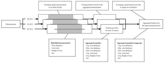
Figure 8.
Feature engineering pipeline that includes spatial and temporal downscaling and aggregation of features.
2.9. Splitting the Dataset
The ratio between training, validation, and testing is set to 70-20-10. This means that 70% of the data is used to train the model, and 20% is used for validation and optimization of the model. To ensure that the model is fully tested for unseen data, and thus to minimize the chance of overfitting, data from certain segments of the railway are completely excluded from the training. After the optimization, the test set of 10% is used to see how the model performs without performance-boosting optimizations.
2.10. Model Training
The machine learning models that are considered are multi-linear regression, random forest, gradient-boosted tree and neural network. For each model type, the Mean Absolute Error (MAE), Mean Squared Error (MSE), Root Mean Squared Error (RMSE) and R-Squared (R2) are measured. These metrics represent the accuracy of the predicted wear rate compared to the actual wear rate. The MAE gives the average absolute difference between the prediction and the actual value. The MSE is the average squared difference between the predicted and actual values. The RMSE is the square root of the MSE which converts the squared difference back into the original unit. The R2 score indicates the percentage of variance between the predicted and actual values. The R2 scores range from 0 to 1, whereby an R2 of 1 means that the predictions are identical to the actual values. In this study, the focus is on the RMSE score when comparing different models.
To determine the long-term performance of the model, the models are tested on a subset of data points. From the data of each block of 10 m, only a portion of the points are used for the prediction. In the example of Figure 9a, the first four data points are used as input for the model. The four data points create the feature values which are used by the model to generate a predicted wear rate, similar to what is shown in Figure 7. These wear rates are projected into the future. In other words, the model does not have any knowledge about what is happening within the ‘prediction horizon’ and is only meant to compare the prediction with the actual values. This is done to make sure the testing of the model is done with a similar scope of input information as the training data.
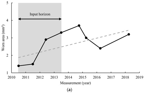
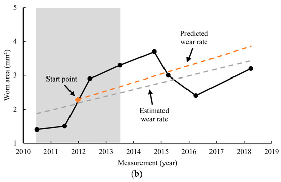
Figure 9.
(a) Selection of limited input horizon and (b) prediction of wear rate and its comparison with the estimated wear rate.
2.11. Conversion of Wear Rate to Worn Area
The model gives a predicted wear rate as an output, as shown in Figure 9b. This predicted wear rate is a single value and appears as a slope when plotted against time. However, for maintenance purposes, the most defining factor is the residual wire area. Therefore, it is important to translate this wear rate back into the current worn area. However, as shown in Figure 9b, for the wear rate to be converted into a worn area, a starting point needs to be determined. This is because the wear rate only implies the slope of the degradation, and in order to be able to determine the worn area, a starting point is needed. This starting point can be either based on measured data or estimated data. If actual measurement data is used, the potential measurement error would have an impact on the prediction of the worn area. However, if an estimated value is used, the random measurement errors can be diluted through data processing (e.g., regression or averaging). In this study, 4 different starting points are tested. The simplest starting point is the last measured worn area within the input horizon (i.e., Point D in Figure 10) and is referred to as the ‘last’ point in the rest of the paper. Because noise can make this last data point unreliable, another alternative can be to first fit a regression line on the data points in the input horizon and then find the last point on this line. This starting point is called the ‘last trend’ and is shown as Point C in Figure 10. The same can be done for the first data point on the fitted line (i.e., Point A in Figure 10), which is labelled as ‘first trend’ hereafter. The last possible starting point can be the average of all the data points in the input horizon. This is shown as Point B in Figure 10.
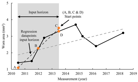
Figure 10.
Different alternatives for the starting point where A indicates the estimated initial worn area, B shows the average of all measurements in the input horizon, C shows the final estimated worn area, and D represents the last measured worn area.
2.12. Assessment of Model Performance
As mentioned before, the defining factor for maintenance is the worn area of the wire. Therefore, it is important to assess the performance of the model in terms of the accuracy of the worn area prediction. To measure the difference between the predicted and estimated worn area, the two values can be compared. This comparison takes place at the latest measurement point, as shown in Figure 11. The estimated worn area is considered to be the actual worn area and is based on the regression line, which is also used as the label of the model. The error of the prediction must be minimized and is quantified by the MAE, MSE, RMSE and R2 metrics.
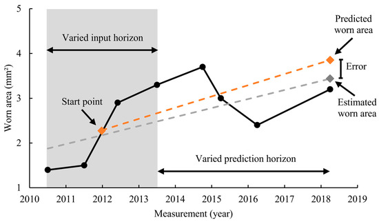
Figure 11.
Calculation of the prediction error.
It should be noted that the further the predictions extend into the future, the greater the errors become. The calculated error depends on the duration of the input horizon and the prediction horizon. For this reason, an experiment is conducted that tests the performance for multiple combinations, as shown in Figure 12. For the experiment, first, a prediction horizon is set. Then, for a given prediction horizon, different input horizons are considered, starting from two data points away from the beginning of the prediction horizon, all the way to the maximum number of possible data points. Following the same principle, different prediction horizons are considered. Figure 12 presents the schematic representation of the scenarios considered in this experiment.
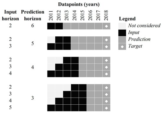
Figure 12.
Schematic representation of different scenarios.
2.13. Clustering Predictions per Wire Section
As mentioned before, the worn area is predicted for every 10 m of the contact wire. However, a single contact wire can have a length of more than a kilometre and will be replaced as a whole. The predictions per 10 m must be combined into a single prediction for the whole wire. For this, the average is calculated based on all predictions within the section. Also, percentiles can be useful for the replacement criteria as the places containing the worst conditions are the defining factors for the life span. Wire sections with less than 5 predictions are removed as these results are unreliable.
3. Results
As mentioned before, the actual measurement data from ProRail (Utrecht, The Netherlands) were used in this research. In total, more than 78 million data points were analyzed in this research. After grouping and filtering the data, 51,080 data points were used for the model development and testing. Table 2 presents ranges of different variables used in this research.
Table 2.
Ranges of different variables in the dataset.
3.1. Performance of the Model for the Prediction of Wear Rate
Four machine learning models were tested in this study to predict the wear rate, as shown in Table 3. This model was trained for the input and prediction horizons of 4 years. As can be seen in this table, linear regression has the best performance with an R2 of 0.682 and is therefore the main model in this study. The random forest model and gradient-boosted tree score worse but still give reasonable results. The neural network model fails to find patterns and cannot give proper predictions. This model type normally performs well when dealing with non-linear data. However, most relationships are linear in this study and the data contains considerable noise. In these cases, more simple models can outperform more complex methods [57].
Table 3.
Performances of different models in terms of wear rate.
Figure 13a presents the scatterplot of the predicted wear rate against the actual wear rate for the linear regression model. As shown in this figure, the predictions have a relatively small error for the lower wear rates. When the wear rate increases, the predictions become slightly less accurate. Figure 13b shows the distributions of errors. The fact that the histogram suggests a normal distribution of errors is an indication that the model captures the overall trend in a balanced manner.
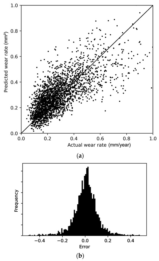
Figure 13.
(a) Scatterplot of the linear regression model showing predicted versus actual wear rates, and (b) Distribution of the wear rate prediction error.
As discussed before, the length of the input horizon has an impact on the accuracy of the model. To test this, the model was tested for different input horizons from 2 to 5 data points. As shown in Table 4, the longer input horizon offered better predictions. It should be noted that only linear regression and random forest are considered, as these models are the best performing.
Table 4.
The impact of input horizon on the prediction of wear rate.
To investigate the contributions of different features to the model, a feature importance analysis was performed for linear regression and random forest models. As can be seen in Figure 14, the linear regression and Random Forest models have different mechanisms. On one hand, Linear regression tends to operate more on the basis of train passages and average/minimum thickness of wires. On the other hand, Random Forest gives marginal importance to train traffic data and instead focuses on the thickness parameters. Both models put the emphasis on the properties of the wire. It should be noted that the feature importance is sensitive to the input horizon. By changing the input horizon, the significance of different features changes slightly. However, the overall trend of which features are more important than others remains constant.
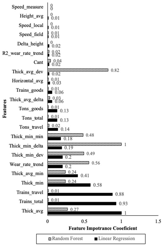
Figure 14.
Feature importance analysis of wear rate prediction for Random Forest and Linear Regression.
3.2. Performance of the Model for the Prediction of Worn Area
As mentioned in Section 2, the worn area is important for maintenance planning. Therefore, the performance of the model needs to be determined for the worn area. As explained in Section 2.11, the translation of wear rate to worn area depends on the selection of an appropriate starting point. To determine the best starting point for the predicted wear rate, the experiment explained in Section 2.11 was conducted. It should be noted that, given the results of wear rate prediction, only linear regression is used for the assessment of the prediction of the worn area. Table 5 presents the RMSE of different starting points. These models are for the cases where 4 data points are used as the input horizon. The starting point that gives the best performance is the average of all the points. Other variations in the starting point produce significantly worse predictions. This starting point is used as the basis of analysis in the rest of this study.
Table 5.
RMSE of worn area prediction for different starting points.
To investigate the impact of the input and prediction horizon on the performance of the model, the experiment presented in Section 2.12 was conducted. As shown in Table 6, generally, the shorter the prediction horizon and the longer the input horizon, the more accurate the prediction of the worn area. This seems very reasonable given that a longer input horizon can better represent the overall wear trend of the wire and this is in line with the observations reported in Section 3.1.
Table 6.
RMSE of worn area prediction of individual predictions for different input and prediction horizons.
Figure 15a shows the scatterplot of the actual against the predicted worn areas for the model that has the input and prediction horizons of 4 years. As shown in this figure, the prediction errors are symmetric. The accuracy of the predictions slightly decreases as the worn area increases. This can be explained by the measurement accuracy. Due to the round shape of the wire, a new wire decreases faster in thickness compared to an older wire. This principle is explained in Figure 4. The accuracy of the measurements is based on the contact area of the wire, which is thus more precise to measure for newer wires.
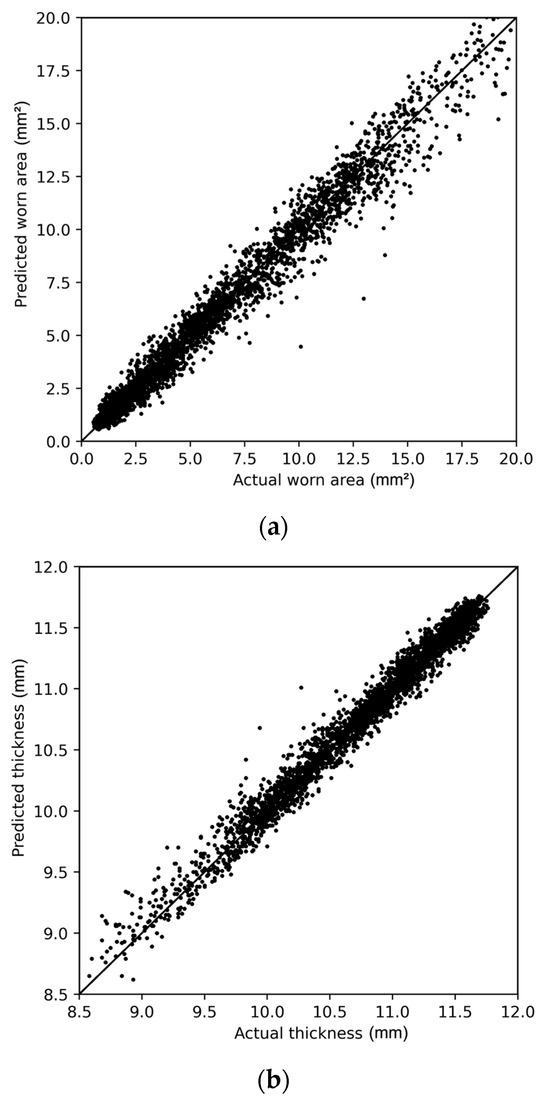
Figure 15.
Scatterplots of predicated vs. actual (a) worn area and (b) thickness.
When the worn area is converted to thickness, the results are easier to interpret. Figure 15b shows the scatterplot of the thickness prediction. It can be seen that most contact wires have a thickness of more than 10 mm. As the predicted thickness is especially important for thinner wires, the predictions for these thin wires need to be accurate. The model has a very slight bias for the thicker wires in the dataset. It is expected that the accuracy for this category can improve if more data from thinner wires is available.
When expressing the accuracy of a model, the confidence level becomes an important factor. For that reason, the accuracy of the model for the prediction of worn area and thickness against different confidence levels was investigated, as shown in Table 7. As can be seen from the scatterplot of Figure 15b, most of the wires are relatively new which results in a better prediction accuracy compared to older wires. The average error is found to be 0.563 mm2 for the worn area and 0.078 mm for the thickness when predicting 4 years into the future.
Table 7.
Accuracy of predictions for different confidence levels.
Finally, as mentioned in Section 2.13, from a practical standpoint, the average thickness of the entire wire is what is considered in maintenance decision-making. Therefore, 10 m sections need to be clustered into individual wires. Because this operation balances out the errors, the overall accuracy is expected to increase. Table 8 shows the analysis of the RMSE of worn area prediction for the entire length of wires. Table 9 presents the overall accuracy of the worn area and thickness predictions for different confidence levels. As is clearly evident from the comparison of Table 6 and Table 8, the accuracy increases considerably when the entire wire is taken into account.
Table 8.
RMSE of worn area prediction of the entire wire for different input and prediction horizons.
Table 9.
Accuracy of predictions for the entire wire considering different confidence levels.
4. Discussion
While the subject of contact wire condition assessment and maintenance, in general, is well-studied in the literature, there is very little research on the use of data-driven modelling approaches for this purpose. This is especially relevant because the recent advancements in information technologies and their ever-growing application in the industry have provided us with a wealth of data that can serve as the basis for modelling and also aid in unravelling the complex wear mechanisms of contact wires, surpassing what can be offered by physics-based models. The primary contribution of this research lies in offering valuable insights into the feasibility and practicality of data-driven models for contact wire condition assessment. The multi-step methodology introduced in this study has demonstrated its effectiveness in the accurate estimation of wire conditions, even when faced with substantial measurement errors, which is an inevitable challenge within the realm of data-driven approaches.
In our analysis, we found that the current thickness consistently emerged as one of the most influential feature categories in all tested models. This finding aligns with the observations made by Takahashi et al. [58] who reported a correlation between residual diameter and local wear rate. Surprisingly, this particular feature is not frequently emphasized in other studies. In theory, converting thickness to worn area should result in a linear wear rate [56]. However, the presence of external factors seems to contradict this theory, leading our model to utilize this feature to account for non-linearity.
Interestingly, our data revealed that new wires experience faster wear, even in terms of worn area, and this non-linearity does not significantly affect our model. When we consider an appropriate timeframe for feature creation and label assignment, the influence of this non-linearity becomes hardly noticeable, likely due to the relatively slow wear of contact wires.
Another notable feature category is the number of passed trains, which intuitively aligns with various wear mechanisms based on pantograph and contact wire interactions. Numerous studies have consistently identified the number of train passages as a key factor contributing to wear and tear [29,31,59]. Conversely, the train speed, a feature often highlighted in prior studies [26,60], did not exhibit a significant correlation with the wear rate in our research. None of the three features approximating actual train speed demonstrated a strong correlation or provided useful information in our model. This divergence from previous findings may be attributed, in part, to the comprehensive nature of our dataset, where constant train speeds prevail on a significant portion of the train tracks. Other features with greater variation throughout the database seem to overshadow the influence of the speed-related features.
Additionally, we employed the total passed tons as a feature to estimate the total electrical current, which proved to be important in modelling wear rates. However, it remains unclear whether this importance stems from capturing total electrical current or if it is related to the number of trains.
For training, all locations with a messy wear pattern have been removed. The wear rate label is created by applying linear regression to the worn area for all data points. The fit of this line is indicated with an R2 score. All R2 scores below 0.4 are filtered out, as this hinders the learning capability of the model. The performance of the model could probably be improved by increasing the minimum R2 score. On the other hand, filtering on R2 scores might create a bias for the model. It is not known if the average thickness of the section can be estimated better by including all cases or by predicting only a part of the cases with higher accuracy. By using low R2 scores, the target also becomes unreliable, which makes it hard to validate the performance.
Another factor that must be taken into account is the presence of carbon deposits. This debris is caused by friction between the contact wire and the pantograph and makes the surface of the contact wire appear wider. The measurement train calculates the thickness of the wire based on the contact surface and interprets a thicker wire if carbon debris is present. This measurement error causes noise and induces a slight deviation in terms of thickness. Besides the carbon deposit, the location of the measurement train is not always accurate. Currently, this problem is mainly solved by clustering the measurements per 10 m. More precise data could be created by applying a synchronization algorithm, which will most likely slightly improve the performance of the model.
The model assumes that the features will stay the same in the future. If it is known that certain values will change in the future and a forecast is available, the values for the features should be updated. If, for example, the number of trains is expected to increase by 10% in the coming years, this percentage can be added to the current value. For instance, for a prediction of 5 years with an expected increase of 10% after 2 years, the average value can be calculated. This would be an average increase of 6% over 5 years, which means that the current feature value should be multiplied by a factor of 1.06 to account for this change.
It should also be noted that due to irregularities in the measurement regime, not all measurements are exactly one year apart. This can be due to any reason, from budgetary constraints, poor measurement planning, varied degrees of tracks’ criticality, and occasionally faulty measurements. While this anomaly in the measurement frequency is only for some limited cases, for the sake of modelling simplicity, we assumed that the temporal distance between all subsequent measurements is always one year. This might have introduced some errors in the results in some minor cases.
The primary goal of this study is to accurately predict the end of the lifetime of a contact wire. This can be done by predicting the average thickness of the whole wire and applying a threshold for the minimum allowed thickness. As the prediction of the wire section consists of many individual predictions, this allows for more complex replacement criteria. Also, percentiles can be used, so that, for example, at least x% of the predicted values must be above a certain thickness threshold. More research can be done to determine which replacement strategy is most suitable.
The measurement train logs the average and minimum thickness measured over a section of 25 cm. Both thickness values can be important to determine the end of the lifetime of the wire. This study focused on the average thickness. However, the same method can be applied to the minimum thickness. The model performance for the average and minimum thickness as labels is almost identical.
It should also be highlighted that the dataset leveraged in this study had a relatively fixed temporal and spatial resolution. Therefore, inherently, the reported performance is sensitive to the availability of the data at the same resolutions. Although the proposed pipeline and the presented framework are not inherently dependent on any particular resolutions, any deviation from the resolution of the dataset in this research will have an effect on the accuracy of the prediction. Conceivably, the lower temporal resolution will provide a small training dataset within a fixed training horizon, and thus the prediction will most likely be less accurate and vice versa. However, the degree and extent of this effect need to be further studied. Also, with respect to the generalizability of the proposed method, the departure point of this research is that periodic thickness measurement is available. If these measurements are available, while there can be some variations in terms of standard material and properties of the wires across different railway contexts, which will impact the wear rate and degradation mechanisms, we strongly believe the proposed method can be applied to all networks as long as sufficiently detailed data are systematically collected and made available.
This study has shown that even with noisy data useful predictions can be generated. This method may also be useful for other assets whereby predictions must be made over a longer period of time. Especially if a lot of noise is present in the data, this method might perform better than most common solutions.
5. Conclusions
The paper presented a novel methodology for the data-driven modelling of contact wire wear mechanisms. The comprehensive methodology comprises multiple steps to systematically deal with the noise in the data and make an accurate prediction of the wire wear rate and worn area. The predictions are made per 10 m and are eventually clustered per wire section. The estimated average thickness of a whole wire has an accuracy of ±0.12 mm at a 95% confidence level, which is very promising.
In general, it can be concluded that the proposed method has a high potential for application in the maintenance of electric train tracks. The greatest challenge in the application of this method is the measurement error and potential inconsistencies in the measurement techniques. However, the multi-step feature engineering method proposed in this research proved to be highly robust.
Despite the promising results, several limitations need to be considered in the future study. In this study, a comprehensive set of features were taken into account, some of which are expected to be correlated. Removing strongly correlated features can potentially improve the performance of the model and also enhance the simplicity and interpretability of the model. The presented predictive model needs to be integrated into a comprehensive maintenance management platform that considers the economical aspect of the different interventions to suggest viable maintenance strategies. Of course, the decision about the maintenance of the wire needs to be combined with the larger maintenance planning of the entire catenary system to avoid rework and additional costs. Therefore, it is important to investigate the maintenance optimization aspect and also integration with the predictive model of other components in the catenary system.
Author Contributions
Conceptualization, J.M., F.V. (Faridaddin Vahdatikhaki) and X.Y.; Methodology, J.M., F.V. (Faridaddin Vahdatikhaki) and X.Y.; Validation, F.V. (Frank Vermeulen); Investigation, J.M.; Writing—original draft, J.M.; Writing—review & editing, F.V. (Faridaddin Vahdatikhaki) and H.V.; Supervision, F.V. (Faridaddin Vahdatikhaki), X.Y., F.V. (Frank Vermeulen) and H.V. All authors have read and agreed to the published version of the manuscript.
Funding
This research received no external funding.
Institutional Review Board Statement
Not applicable.
Informed Consent Statement
Not applicable.
Data Availability Statement
Data were obtained from ProRail and are not publicly available due to confidentiality agreements.
Acknowledgments
The authors have reviewed and edited the output and take full responsibility for the content of this publication.
Conflicts of Interest
The authors declare no conflict of interest.
References
- Zeng, Y.; Qin, Y.; Liu, D.; Fu, Y.; Gong, M.; Zhang, X. Railway Train Device Fault Causality Model Based on Knowledge Graph. In Proceedings of the 2020 International Conference on Sensing, Diagnostics, Prognostics, and Control, SDPC, Beijing, China, 5–7 August 2020; pp. 385–390. [Google Scholar] [CrossRef]
- Jing, G.; Qin, X.; Wang, H.; Deng, C. Developments, challenges, and perspectives of railway inspection robots. Autom. Constr. 2022, 138, 104242. [Google Scholar] [CrossRef]
- Grandio, J.; Riveiro, B.; Lamas, D.; Arias, P. Multimodal deep learning for point cloud panoptic segmentation of railway environments. Autom. Constr. 2023, 150, 104854. [Google Scholar] [CrossRef]
- Sedghi, M.; Kauppila, O.; Bergquist, B.; Vanhatalo, E.; Kulahci, M. A taxonomy of railway track maintenance planning and scheduling: A review and research trends. Reliab. Eng. Syst. Saf. 2021, 215, 107827. [Google Scholar] [CrossRef]
- Vithanage, R.K.W.; Harrison, C.S.; Desilva, A.K.M. Importance and Applications of Robotic and Autonomous Systems (RAS) in Railway Maintenance Sector: A Review. Computers 2019, 8, 56. [Google Scholar] [CrossRef]
- Stenström, C.; Norrbin, P.; Parida, A.; Kumar, U. Preventive and corrective maintenance—Cost comparison and cost–benefit analysis. Struct. Infrastruct. Eng. 2016, 12, 603–617. [Google Scholar] [CrossRef]
- Zhang, D.; Hu, H.; Roberts, C. Rail maintenance analysis using Petri nets. Struct. Infrastruct. Eng. 2017, 13, 783–793. [Google Scholar] [CrossRef]
- Xie, J.; Huang, J.; Zeng, C.; Jiang, S.H.; Podlich, N. Systematic Literature Review on Data-Driven Models for Predictive Maintenance of Railway Track: Implications in Geotechnical Engineering. Geosciences 2020, 10, 425. [Google Scholar] [CrossRef]
- Bukhsh, Z.A.; Saeed, A.; Stipanovic, I.; Doree, A.G. Predictive maintenance using tree-based classification techniques: A case of railway switches. Transp. Res. Part C Emerg. Technol. 2019, 101, 35–54. [Google Scholar] [CrossRef]
- Sanjrani, A.N.; Huang, H.Z.; Shah, S.A.; Hussain, F.; Punhal, M.; Narejo, A.; Zhang, B. High-speed train wheel set bearing analysis: Practical approach to maintenance between end of life and useful life extension assessment. Results Eng. 2025, 25, 103696. [Google Scholar] [CrossRef]
- Cheng, M.Y.; Khasani, R.R.; Setiono, K. Image quality enhancement using HybridGAN for automated railway track defect recognition. Autom. Constr. 2023, 146, 104669. [Google Scholar] [CrossRef]
- Wang, X.; Bai, Y.; Liu, X. Prediction of railroad track geometry change using a hybrid CNN-LSTM spatial-temporal model. Adv. Eng. Inform. 2023, 58, 102235. [Google Scholar] [CrossRef]
- Sharma, S.; Cui, Y.; He, Q.; Mohammadi, R.; Li, Z. Data-driven optimization of railway maintenance for track geometry. Transp. Res. Part C Emerg. Technol. 2018, 90, 34–58. [Google Scholar] [CrossRef]
- Poyyamozhi, M.; Devadharshini, A.S.K.; Murugesan, B.; Novak, T.; Mlcak, T.; R, N. Enhancing railway track maintenance with real-time ultrasonic and moisture sensing: Proactive and zone-specific management strategies. Results Eng. 2024, 24, 103472. [Google Scholar] [CrossRef]
- Haroon, M.; Khan, M.J.; Cheema, H.M.; Nasir, M.T.; Safdar, M.; Butt, S.I.U. An end-to-end approach to detect railway track defects based on supervised and self-supervised learning. Results Eng. 2024, 24, 103326. [Google Scholar] [CrossRef]
- Wu, Y.; Qin, Y.; Qian, Y.; Guo, F. Automatic detection of arbitrarily oriented fastener defect in high-speed railway. Autom. Constr. 2021, 131, 103913. [Google Scholar] [CrossRef]
- Meng, F.; Qin, Y.; Wu, Y.; Shao, C.; Jia, L. A subtle defect recognition method for catenary fastener in high-speed railroad using destruction and reconstruction learning. Adv. Eng. Inform. 2024, 60, 102393. [Google Scholar] [CrossRef]
- Xu, R.H.; Lai, Y.C.; Huang, K.L. Decision support models for annual catenary maintenance task identification and assignment. Transp. Res. Part E Logist. Transp. Rev. 2021, 152, 102402. [Google Scholar] [CrossRef]
- Lin, S.; Li, N.; Sun, X.; Feng, D. Research on Maintenance Efficiency Optimization for the Catenary System of Electrified Railways. In Proceedings of the 2021 IEEE IAS Industrial and Commercial Power System Asia, I and CPS Asia, Chengdu, China, 18–21 July 2021; pp. 942–947. [Google Scholar] [CrossRef]
- Adeagbo, M.O.; Wang, S.M.; Ni, Y.Q. Revamping structural health monitoring of advanced rail transit systems: A paradigmatic shift from digital shadows to digital twins. Adv. Eng. Inform. 2024, 61, 102450. [Google Scholar] [CrossRef]
- Lin, S.; Shang, C.; Li, N.; Sun, X.; Feng, D.; He, Z. An Optimization Method for Maintenance Resource Allocation in Electrified Railway Catenary Systems. IEEE Trans. Ind. Appl. 2023, 59, 641–651. [Google Scholar] [CrossRef]
- Li, L.; Mahmoodian, M.; Khaloo, A. Service life prediction of worn contact wires under multiple failure modes. Struct. Infrastruct. Eng. 2023, 19, 1530–1541. [Google Scholar] [CrossRef]
- Rauter, F.G.; Pombo, J.; Ambrósio, J.; Chalansonnet, J.; Bobillot, A.; Pereira, M.S. Contact Model for The Pantograph-Catenary Interaction. J. Syst. Des. Dyn. 2007, 1, 447–457. [Google Scholar] [CrossRef]
- Philippov, V.; Smerdin, A. Modeling the mechanical wear of the contact elements of pantograph during high-speed movement. E3S Web Conf. 2020, 157, 01022. [Google Scholar] [CrossRef]
- Song, Y.; Rønnquist, A.; Jiang, T.; Nåvik, P. Identification of short-wavelength contact wire irregularities in electrified railway pantograph–catenary system. Mech. Mach. Theory 2021, 162, 104338. [Google Scholar] [CrossRef]
- Wei, X.K.; Meng, H.F.; He, J.H.; Jia, L.M.; Li, Z.G. Wear analysis and prediction of rigid catenary contact wire and pantograph strip for railway system. Wear 2020, 442–443, 203118. [Google Scholar] [CrossRef]
- Derosa, S.; Nåvik, P.; Collina, A.; Bucca, G.; Rønnquist, A. A heuristic wear model for the contact strip and contact wire in pantograph—Catenary interaction for railway operations under 15 kV 16.67 Hz AC systems. Wear 2020, 456–457, 203401. [Google Scholar] [CrossRef]
- Usuda, T. Estimation of Wear and Strain of Contact Wire Using Contact Force of Pantograph. Q. Rep. RTRI 2007, 48, 170–175. [Google Scholar] [CrossRef]
- Shing, W.C. A Survey of Contact Wire Wear Parameters and the Development of a Model to Predict Wire Wear by Using the Artifical Neural Network. Ph.D. Thesis, City University of Hong Kong, Kowloon, Hong Kong, 2011. [Google Scholar]
- Jia, S.G.; Liu, P.; Ren, F.Z.; Tian, B.H.; Zheng, M.S.; Zhou, G.S. Sliding wear behavior of copper alloy contact wire against copper-based strip for high-speed electrified railways. Wear 2007, 262, 772–777. [Google Scholar] [CrossRef]
- Wang, H.; Núñez, A.; Liu, Z.; Song, Y.; Duan, F.; Dollevoet, R. Analysis of the evolvement of contact wire wear irregularity in railway catenary based on historical data. Veh. Syst. Dyn. 2018, 56, 1207–1232. [Google Scholar] [CrossRef]
- Serradilla, O.; Zugasti, E.; Rodriguez, J.; Zurutuza, U. Deep learning models for predictive maintenance: A survey, comparison, challenges and prospects. Appl. Intell. 2022, 52, 10934–10964. [Google Scholar] [CrossRef]
- Namuduri, S.; Narayanan, B.N.; Davuluru, V.S.P.; Burton, L.; Bhansali, S. Review—Deep Learning Methods for Sensor Based Predictive Maintenance and Future Perspectives for Electrochemical Sensors. J. Electrochem. Soc. 2020, 167, 037552. [Google Scholar] [CrossRef]
- Hassan, M.U.; Steinnes, O.M.H.; Gustafsson, E.G.; Løken, S.; Hameed, I.A. Predictive Maintenance of Norwegian Road Network Using Deep Learning Models. Sensors 2023, 23, 2935. [Google Scholar] [CrossRef]
- Lv, Y.; Guo, X.; Zhou, Q.; Qian, L.; Liu, J. Predictive maintenance decision-making for variable faults with non-equivalent costs of fault severities. Adv. Eng. Inform. 2023, 56, 102011. [Google Scholar] [CrossRef]
- Sahba, R.; Radfar, R.; Ghatari, A.R.; Ebrahimi, A.P. Development of Industry 4.0 predictive maintenance architecture for broadcasting chain. Adv. Eng. Inform. 2021, 49, 101324. [Google Scholar] [CrossRef]
- Yucesan, Y.A.; Dourado, A.; Viana, F.A.C. A survey of modeling for prognosis and health management of industrial equipment. Adv. Eng. Inform. 2021, 50, 101404. [Google Scholar] [CrossRef]
- Liu, X.; Cheng, W.; Xing, J.; Chen, X.; Li, L.; Guan, Y.; Ding, B.; Nie, Z.; Zhang, R.; Zhi, Y. Predictive maintenance system for high-end equipment in nuclear power plant under limited degradation knowledge. Adv. Eng. Inform. 2024, 61, 102506. [Google Scholar] [CrossRef]
- Li, H.; Parikh, D.; He, Q.; Qian, B.; Li, Z.; Fang, D.; Hampapur, A. Improving rail network velocity: A machine learning approach to predictive maintenance. Transp. Res. Part C Emerg. Technol. 2014, 45, 17–26. [Google Scholar] [CrossRef]
- Tang, R.; De Donato, L.; Bes, N.; Flammini, F.; Goverde, R.M.P.; Lin, Z.; Liu, R.; Tang, T.; Vittorini, V.; Wang, Z. A literature review of Artificial Intelligence applications in railway systems. Transp. Res. Part C Emerg. Technol. 2022, 140, 103679. [Google Scholar] [CrossRef]
- Xu, Y.; Fan, Y.; Bao, Y.; Li, H. Few-shot learning for structural health diagnosis of civil infrastructure. Adv. Eng. Inform. 2024, 62, 102650. [Google Scholar] [CrossRef]
- Gao, Z.; Chen, N.; Yang, Y.; Li, L. An innovative multisource multibranch metric ensemble deep transfer learning algorithm for tool wear monitoring. Adv. Eng. Inform. 2024, 62, 102659. [Google Scholar] [CrossRef]
- Nampalli, R.C.R. Leveraging AI and Deep Learning for Predictive Rail Infrastructure Maintenance: Enhancing Safety and Reducing Downtime. Int. J. Eng. Comput. Sci. 2023, 12, 26014–26027. [Google Scholar] [CrossRef]
- Davari, N.; Veloso, B.; Ribeiro, R.P.; Pereira, P.M.; Gama, J. Predictive maintenance based on anomaly detection using deep learning for air production unit in the railway industry. In Proceedings of the 2021 IEEE 8th International Conference on Data Science and Advanced Analytics, DSAA, Porto, Portugal, 6–9 October 2021. [Google Scholar] [CrossRef]
- MajidiParast, S.; Monemi, R.N.; Gelareh, S. A graph convolutional network for optimal intelligent predictive maintenance of railway tracks. Decis. Anal. J. 2025, 14, 100542. [Google Scholar] [CrossRef]
- Huang, G.; Wu, G.; Yang, Z.; Chen, X.; Wei, W. Development of surrogate models for evaluating energy transfer quality of high-speed railway pantograph-catenary system using physics-based model and machine learning. Appl. Energy 2023, 333, 120608. [Google Scholar] [CrossRef]
- Gregori, S.; Tur, M.; Gil, J.; Fuenmayor, F.J. Assessment of catenary condition monitoring by means of pantograph head acceleration and Artificial Neural Networks. Mech. Syst. Signal Process. 2023, 202, 110697. [Google Scholar] [CrossRef]
- Kuźnar, M.; Lorenc, A. A Method of Predicting Wear and Damage of Pantograph Sliding Strips Based on Artificial Neural Networks. Materials 2021, 15, 98. [Google Scholar] [CrossRef]
- Blanco, B.; Errandonea, I.; Beltrán, S.; Arrizabalaga, S.; Alvarado, U. Panhead accelerations-based methodology for monitoring the stagger in overhead contact line systems. Mech. Mach. Theory 2022, 171, 104742. [Google Scholar] [CrossRef]
- Phala, K.; Doorsamy, W.; Paul, B.S. An Intelligent Fault Monitoring System for Railway Neutral Sections. In Proceedings of International Conference on Communication and Computational Technologies; Springer: Singapore, 2021; pp. 835–844. [Google Scholar] [CrossRef]
- Yang, J.; Duan, H.; Li, L.; Stewart, E.; Huang, J.; Dixon, R. 1D CNN Based Detection and Localisation of Defective Droppers in Railway Catenary. Appl. Sci. 2023, 13, 6819. [Google Scholar] [CrossRef]
- Kuźnar, M.; Lorenc, A.; Kaczor, G. Pantograph Sliding Strips Failure—Reliability Assessment and Damage Reduction Method Based on Decision Tree Model. Materials 2021, 14, 5743. [Google Scholar] [CrossRef]
- Alkam, F.; Lahmer, T. A robust method of the status monitoring of catenary poles installed along high-speed electrified train tracks. Results Eng. 2021, 12, 100289. [Google Scholar] [CrossRef]
- Gbadamosi, A.Q.; Oyedele, L.O.; Delgado, J.M.D.; Kusimo, H.; Akanbi, L.; Olawale, O.; Muhammed-yakubu, N. IoT for predictive assets monitoring and maintenance: An implementation strategy for the UK rail industry. Autom. Constr. 2021, 122, 103486. [Google Scholar] [CrossRef]
- Moussallik, L. Towards Condition-Based Maintenance of Catenary Wires Using Computer Vision. Master’s Thesis, Luleå University of Technology, Luleå, Sweden, 2021. [Google Scholar]
- Archard, J.F. Contact and Rubbing of Flat Surfaces. J. Appl. Phys. 1953, 24, 981–988. [Google Scholar] [CrossRef]
- Kuhn, M.; Johnson, K.; Modeling, A.P. Springer. 2013. Available online: http://ir.mksu.ac.ke/handle/123456780/6225 (accessed on 2 November 2023).
- Takahashi, A.; Kishi, T.; Yamamoto, H. Overhead Contact Line Monitoring and Prediction of Contact Wire Localized Wear Points. JR East Tech. Rev. 2014, 29, 22–25. [Google Scholar]
- Bucca, G.; Collina, A. A procedure for the wear prediction of collector strip and contact wire in pantograph–catenary system. Wear 2009, 266, 46–59. [Google Scholar] [CrossRef]
- Bucca, G.; Collina, A. Electromechanical interaction between carbon-based pantograph strip and copper contact wire: A heuristic wear model. Tribol. Int. 2015, 92, 47–56. [Google Scholar] [CrossRef]
Disclaimer/Publisher’s Note: The statements, opinions and data contained in all publications are solely those of the individual author(s) and contributor(s) and not of MDPI and/or the editor(s). MDPI and/or the editor(s) disclaim responsibility for any injury to people or property resulting from any ideas, methods, instructions or products referred to in the content. |
© 2025 by the authors. Licensee MDPI, Basel, Switzerland. This article is an open access article distributed under the terms and conditions of the Creative Commons Attribution (CC BY) license (https://creativecommons.org/licenses/by/4.0/).