Article

A Freight Train Optimized Scheduling Scheme Based on an Improved GJO Algorithm

1
School of Traffic and Transportation, Beijing Jiaotong University, Beijing 100044, China
2
School of Electrical and Information Engineering, Zhengzhou University of Light Industry, Zhengzhou 450002, China
*
Author to whom correspondence should be addressed.
Appl. Sci. 2025, 15(17), 9326; https://doi.org/10.3390/app15179326 (registering DOI)
Submission received: 14 July 2025 / Revised: 17 August 2025 / Accepted: 19 August 2025 / Published: 25 August 2025

Abstract

With the advancement of China’s industrialization, demand for express freight transportation has been rising. However, high-speed rail freight faces challenges, such as relatively low transport efficiency and lower revenues, compared with air and road modes. To address these issues, this paper focuses on freight train operations. First, it analyzes key influencing factors, including operating costs and benefits. Next, it conducts a comprehensive assessment of train consist capacity, freight node capacity, transport demand, and the number of freight services, and formulates an operational planning model that maximizes rail revenue, minimizes intermediate stops, and satisfies freight demand. Finally, an Improved Golden Jackal Optimization–based Genetic Algorithm (IGJOGA) is proposed to solve the model. Simulation results indicate that IGJOGA achieves higher solution efficiency than a traditional genetic algorithm for the freight train operation planning problem, and the results can provide a practical reference for freight train set operation schemes.

1. Introduction

The rapid development of China’s industrialization and the Internet has led to a substantial rise in demand for high value-added products in express cargo and commodity logistics. These products—primarily electronics, machinery, and foodstuffs—require highly efficient transportation. At present, most shipments still rely on highways and air transport [1]. Highway transport is slower and has limited carrying capacity, while air transport, though faster, is more expensive and susceptible to weather and other uncertainties. As an emerging mode for high value-added cargo, high-speed rail can address the shortcomings of both [2]. With the ongoing construction of high-speed rail lines, an intercity high-speed rail network is gradually taking shape, providing significant transport capacity between cities [3]. High-speed rail networks are designed to meet the time, safety, and cost requirements of high value-added freight. China’s rail network is projected to reach 200,000 km by 2035, ultimately achieving 80% national coverage [4]. Therefore, using high-speed rail to transport high value-added goods is a highly viable option.
Given the scale and complexity of high-speed rail freight, achieving integrated planning and rational operations across the rail system is challenging. Consequently, many scholars have explored mathematical models and optimization techniques to improve rail operations. Archetti et al. examined the effects of different intermodal configurations on freight trains and argued that future transport systems should move toward synchronized operations [5]. Hosseini et al. developed a new intermodal network integrating road, water, and rail, and used the model to determine optimal routes and rerouting strategies for system-wide freight transport during and after disasters [6]. Smolyanivov et al. applied a SWOT analysis to the development of piggybacking in rail networks, demonstrating that this mode can enhance the efficiency of transport infrastructure [7].
While prior research has largely focused on freight train transportation modes, the rail system must also sustain high operational efficiency to enhance competitiveness and improve carrier performance [8]. Consequently, scholars have begun to emphasize the transportation efficiency of freight trains. Jaramillo et al. employed supervised machine learning with classification algorithms to predict delay durations caused by disruptions in multi-modal transport, showing that longer and heavier trains are more prone to delays [9]. Li et al. developed a train path optimization model to reduce total travel time and ensure on-time delivery [10]. Wang et al. proposed an integer programming model that minimizes total costs—including service- and distance-based components—and solved it using a tabu search algorithm, demonstrating reductions in the number of shift-service vehicles required [11]. Although these studies improve the transportation and service efficiency of freight trains, the central challenge for high-speed rail freight remains maximizing the operating companies’ benefits while satisfying constraints on train size.
This paper investigates the freight train operation planning problem using five inland city nodes in China as a case study. It conducts a comprehensive analysis of onboard train capacity, freight node capacity, transport demand, and the number of freight services, among other factors. The proposed planning model seeks to maximize revenue, minimize the number of intermediate stops, and satisfy freight demand. To solve the model, an Improved Golden Jackal Optimizer–based Genetic Algorithm (IGJOGA) is employed. The Genetic Algorithm (GA) is a parallel search method inspired by natural selection [12] and has been successfully applied in fields such as artificial intelligence [13], UAV path planning [14], and fuzzy PID control [15]. However, as a generalized stochastic search algorithm, GA can suffer from premature convergence and slow convergence when tackling the freight train operation planning problem. To address these limitations, this paper proposes an Improved Golden Jackal Optimizer (IGJO) and integrates it with GA to solve the freight train operation scheduling model.
The contributions of this paper are as follows:
(1)
We develop a freight train operation planning model with multiple objectives: maximizing enterprise operational efficiency, optimizing the number of services, minimizing intermediate stops, and accounting for train operational costs.
(2)
We propose a novel Improved Golden Jackal Optimizer-based Genetic Algorithm (IGJOGA) to solve the freight train operation planning model.
(3)
We verify the feasibility and effectiveness of the improved strategy through CEC2022 benchmark function tests and operational simulations. The experimental results demonstrate that the proposed algorithm effectively overcomes the limitations of the traditional GA, enabling freight trains to operate with maximum efficiency.

2. Description of the Problem

Currently, high-speed rail cargo is primarily transported via two schemes: Daily Confirmed Trains [16] and mixed passenger–freight services [17]. In the Daily Confirmed Train scheme, the first confirmed service of the day is allocated to carry freight. In mixed passenger–freight operations, spare capacity on passenger trains is utilized for cargo. However, both approaches suffer from limited freight capacity, making it difficult to accommodate large shipment volumes [18].
Freight trainsets operating with point-to-point loading–unloading services can expand intercity freight capacity and generate substantial social and economic benefits [19]. This paper adopts the perspective of freight transport enterprises, using trainset operational efficiency as a key performance indicator. From a business standpoint, effectiveness hinges on costs and revenues. The costs of freight trains comprise direct and indirect expenses. Direct costs include per-kilometer operating expenses, line access charges, and locomotive traction costs, while indirect costs cover station technical operations and the maintenance of associated equipment. Revenue is typically accounted for on a per train-kilometer basis [20]. Accordingly, the optimization of the freight train operation scheme centers on leveraging spare capacity in the high-speed rail network to enhance rail freight efficiency.

3. Freight Train Departure Scheme Model

3.1. Basic Assumption

This paper adopts a point-to-point operating mode for freight trains. In formulating the freight train operation plan, we consider the interests of transport enterprises, service frequency, and trainset grouping (consist formation). To simplify the problem, we make the following assumptions:
(1)
The freight train path is defined as the shortest route from origin (O) to destination (D). We assume that cost parameters, timetable punctuality, and the O–D pairs remain fixed.
(2)
Trains carry only general cargo; commodities prohibited on high-speed lines (e.g., hazardous or restricted goods) are excluded.
(3)
Freight demands at nodes along the route are known and time-invariant.
(4)
Section headways and node handling capacities are computed under nominal conditions, without accounting for dynamic dispatching, maintenance windows, or other operational adjustments.
(5)
Trains adopt a passenger-style fixed-consist operating mode with high priority; exact departure/arrival timing is not modeled, and overtakes between passenger and freight trains are not considered.
(6)
All nodes traversed by the freight trains are freight-only facilities; passenger services and other functions are not modeled.

3.2. Description of Symbols in the Model

To establish an optimization model for the freight train operation scheme, it is necessary to describe the formulas and variables involved in the model. By knowing the location of each node in the high-speed railroad network, the resources between nodes can be calculated using the given formula. This paper defines sets, parameters, and decision variables.

3.2.1. Set Definition

(1)
S is denoted as the set of stations in the freight train network, s S .
(2)
I denotes the originating city of the freight train, i I .
(3)
J denotes the arrival city of the freight train, j J ; i j , I = J .
(4)
E denotes the set of segments in the railroad network, e E .
(5)
Q denotes the set of freight demand between nodes in the railroad network, q Q .
(6)
K denotes the number of trains a train can run per day, k K .

3.2.2. Parameter Definition

(1)
n ( e ) denotes the freight train running on the section e .
(2)
n i , j k denotes the number of cars loaded by freight train k from platform S i to platform S j .
(3)
Q i , j denotes the predicted value of the cargo flow of a freight train from platform S i to platform S j .
(4)
d i , j denotes the distance between the freight train at the platform S i to the platform S j .
(5)
C 1 is the average operating revenue per ton-kilometer for freight trains.
(6)
C 2 is the operating cost of the train per kilometer, including line usage and locomotive traction costs.
(7)
C 3 is the cost required for technical operations at stations.
(8)
q i , j denotes the average number of tons loaded in each car of a freight train from platform S i to platform S j .

3.2.3. Decision Variables

x m k denotes the stopping of the train at station m. When x m k takes the value 0, it means no stop, and when x m k takes the value 1, it means stop.

3.3. Objective Function

The objective of this study is to maximize the efficiency of the freight-forwarding company, defined as operating profit (revenue minus cost). Accordingly, the objective function comprises two components: operating revenue and operating cost. Operating revenue is computed primarily from the freight tariff, that is, the transportation revenue per kilometer of cargo delivered by a freight train. Operating costs include both direct and indirect components. Direct costs consist of per-kilometer operating expenses, line-access charges, and locomotive traction costs, while indirect costs include station technical operations and equipment maintenance. Accordingly, the objective function is as follows:
m a x Z = Z r Z c
where Z r is the operating revenue, and Z c is the operating cost.
Z r = C 1 i = 1 n j = 2 n 1 k = 1 K q i , j d i , j n i , j k
Z c = Z d + Z i
where Z d is the direct cost, and Z i is the indirect cost.
Z d = C 2 i = 1 n j = 2 n 1 k = 1 K q i , j d i , j n i , j k
Z i = C 3 k = 1 K x m k
In summary, the objective function of maximizing the efficiency of freight transport companies can be expressed as follows:
m a x Z = C 1 C 2 i = 1 n j = 2 n 1 k = 1 K q i , j d i , j n i , j k C 3 k = 1 K x m k

3.4. Constraints

The operation of freight trains is also subject to the following constraints.
(1)
Freight demand constraint
i = 1 n j = 2 n 1 k = 1 K q i , j n i , j k Q i , j
(2)
Freight train stop constraints
x m k is the stopping of the freight train at station m . When x m k takes the value 0, it means no stop, and when x m k takes the value 1, it means stop. The maximum number of stops, other than the starting station, cannot exceed n 2 . Additionally, the constraint that the train must stop at least one node station for loading and unloading operations should also be satisfied.
1 k = 1 K x m k n 2
k = 1 K x m k = 0 , o r , k = 1 K x m k = 1
(3)
Loading constraint
To ensure efficient operational gains, freight trains need to be loaded to a specific value.
0 < q < L
where L denotes the maximum loading capacity of a single train.

4. Algorithm Design

Traditional methods for solving the correlation model often suffer from limited solution accuracy and low computational efficiency [17]. Genetic algorithms (GAs) offer strong inherent parallelism for objective-function evaluation; however, their solution accuracy can still be inadequate [21]. The GJO algorithm, proposed by Chopra and Ansari in 2022, is a swarm-based metaheuristic characterized by a small number of parameters and a simple structure [22]. Nevertheless, GJO is susceptible to premature convergence and entrapment in local optima [23]. To leverage their complementary strengths, we combine GJO with GA, resulting in a hybrid approach that retains high solution efficiency while mitigating local-optimum pitfalls and improving solution quality for the objective considered in this study.

4.1. Coding Approach

Each chromosome in the GA represents a solution to the problem, and coding is the method by which the problem’s solution is converted into a format that the GA can process. In other words, encoding involves converting the traditional decimal method into a binary format. Using this encoding, selection, cross-over, and mutation operations are applied, and ultimately, the optimal solution to the problem can be obtained after decoding.

4.2. Fitness Function

The objective function described in Section 3.3 of this paper, to maximize the benefits of freight trains, is designed as the fitness function of the algorithm. Its expression is shown below:
m a x Z = C 1 C 2 i = 1 n j = 2 n 1 k = 1 K q i , j d i , j n i , j k C 3 k = 1 K x m k

4.3. Selection

The selection operation involves selecting the optimal individual from the population and transferring it to the next generation. This approach enables the algorithm to move in a more advantageous direction. There are three commonly used approaches to selection operations: the roulette wheel, the ranked selection, and the optimal strategy preservation method. In this paper, the roulette wheel method is used, where the selection probability is positively correlated with the fitness function. The specific expression is as follows:
p i = f i i f i
where f i denotes the fitness of the i -th parent individual.

4.4. Cross-Over Operation

The cross-over operation randomly selects individuals from the parent generation and crosses them over to produce a new chromosome. Commonly used cross-over methods include single-point, double-point, and multi-point cross-overs. This paper uses the single-point cross-over method, and the chromosome cross-over schematic is shown in Figure 1.

4.5. Mutation Operation

The mutation operation is an essential method for genetic algorithms to maintain diversity, which simulates the phenomenon of genetic mutation during the evolution of species. In this paper, a segment is randomly selected, and a mutation operation is performed on it. The schematic diagram of the mutation process is shown in Figure 2.

4.6. Improved Golden Jackal Optimizer-Based Genetic Algorithm

The GA has the problem of falling into local optima after selection, cross-over, and mutation operations. Therefore, IGJO has been added to enhance the efficiency of the algorithm solution.

4.6.1. Golden Jackal Optimization Algorithm

Like its heuristic algorithm, GJO is a swarm-based method. The initial candidate solutions are randomly generated in the solution space using the following mathematical formulation:
Y 0 = Y L + r a n d ( Y U Y L )
where Y L and Y U denote the previous and next sessions in the solution space, respectively; $rand$ denotes any number between 0 and 1.
The initial position matrix of the ‘Prey’ is as follows:
P r e y = Y 1 , 1 Y 1 , 2 Y 1 , d Y 2 , 1 Y 2 , 2 Y 2 , d Y n , 1 Y n , 2 Y n , d
where Y i , j denotes the j -th dimension of the i -th prey; n and d are denoted as the total number of prey and the size of the dimension in the search space.
The fitness matrix is expressed as follows:
H O A = f ( Y 1 , 1 Y 1 , 2 Y 1 , d ) f ( Y 2 , 1 Y 2 , 2 Y 2 , d ) f ( Y n , 1 Y n , 2 Y n , d )
where H O A denotes the fitness matrix containing all prey, and f denotes the objective function.
Rank all fitness values in the search space. The individual with the best fitness value is called the male jackal, and the individual with the second-best fitness value is called the female jackal. The activities in the exploration phase are led by the male jackal, and the female jackal follows the male jackal in searching for prey. The equation for the exploration process is as follows:
Y 1 ( t ) = Y M ( t ) E | Y M ( t ) r l P r e y ( t ) |
Y 2 ( t ) = Y F M ( t ) E | Y F M ( t ) r l P r e y ( t ) |
where t denotes the current number of iterations; ‘Prey’ denotes the current prey position; Y M and Y F M denote the positions of male and female jackals, respectively; Y 1 denotes the updated position of the male jackal; Y 2 denotes the updated position of the female jackal.
E denotes the escape energy of the prey, which is calculated as follows:
E = E 1 E 0
where E 1 denotes the decreasing energy of the prey; E 0 denotes the initial energy of the prey.
E 0 = 2 R 1
E 1 = a 1 ( 1 ( t / T ) )
where R denotes a random number between 0 and 1; a 1 is a constant, and a 1 = 1.5 ; t denotes the number of current iterations; T denotes the maximum number of iterations.
In Equations (16) and (17), r l denotes the random vector using the Lévy flight distribution with the following expression:
r l = 0.05 L F ( z )
L F ( z ) = 0.01 × ( μ × σ )   / ( | v ( 1 / β ) | ) ; σ = Γ ( 1 + β ) × sin ( π × β 2 ) Γ ( 1 + β 2 ) × β × ( 2 β 1 2 ) 1 β
where μ and v denote random numbers between 0 and 1, respectively; β is a default constant taking the value 1.5. Finally, the position update is performed using the following equation:
Y ( t + 1 ) = Y 1 ( t ) + Y 2 ( t ) 2
When the prey is harassed by a jackal, the energy E will drop. At this point, the jackal pounces on the prey and eats it. The mathematical expression for this phase is as follows:
Y 1 ( t ) = Y M ( t ) E | r l Y M ( t ) P r e y ( t ) |
Y 2 ( t ) = Y F M ( t ) E | r l Y F M ( t ) P r e y ( t ) |
where t denotes the current number of iterations; P r e y ( t ) denotes the position vector of the prey; Y M and Y F M denote the positions of the male jackal and female jackal; Y 1 and Y 2 denote the next updated positions of the male jackal and female jackal.
In GJO technology, the transition from exploration to exploitation by the golden jackal is based on the energy E of the prey. When E < 1 , the jackal attacks the prey. When E > 1 , the jackal will search for the prey again.

4.6.2. Improved the Golden Jackal Optimization Algorithm

The GJO algorithm features conceptual simplicity, few parameters, and strong performance in unknown search spaces. Nevertheless, it remains susceptible to premature convergence and entrapment in local optima. To address this, we introduce two enhancements: (i) an adaptive weighting strategy that strengthens the algorithm’s optimization capability, and (ii) a t-distribution–based variation strategy that bolsters the golden jackal’s global exploration ability.
(1)
Adaptive weighting strategy
The adaptive weighting strategy is a critical component of the optimization algorithm. In general, larger weights enhance the algorithm’s search capability, whereas smaller weights weaken it. This paper proposes a new adaptive weighting method: during the GJO exploration phase, a smaller weight is assigned so that the golden jackal maintains a small distance from the prey’s position; during the exploitation phase, a larger weight is used to drive the golden jackal rapidly toward the prey, thereby improving the algorithm’s optimization capability. The adaptive weighting formula is given in Equation (26).
w = t T × sin t 2 × T + π
The position update equation after adding adaptive weights is shown below:
Y 1 ( t ) = Y M ( t ) E | Y M ( t ) w r l P r e y ( t ) | Y 2 ( t ) = Y F M ( t ) E | Y F M ( t ) w r l P r e y ( t ) |
Y 1 ( t ) = Y M ( t ) E | w r l Y M ( t ) P r e y ( t ) | Y 2 ( t ) = Y F M ( t ) E | w r l Y F M ( t ) P r e y ( t ) |
(2)
t-distribution mutation strategy
The t-distribution, also known as the “student distribution”, contains degrees of freedom n . When t ( n ) N ( 0 , 1 ) and t ( n = 1 ) C ( 0 , 1 ) , N ( 0 , 1 ) is a Gaussian distribution, and C ( 0 , 1 ) is a Cauchy distribution.
In this paper, we use the number of iterations instead of the degree of freedom N to mutate the position of the golden jackal. This method allows the algorithm to better develop globally in the early stage and enhance the local search capability of the algorithm later in the iteration. The t-distribution position update formula is as follows:
Y ( t + 1 ) = Y M ( t ) + Y M ( t ) t ( i t e r )
where Y ( t + 1 ) is the position after mutation; Y M ( t ) is the optimal position of the golden jackal; i t e r is the current number of iterations, and t ( ) is the t-distribution function.
As the number of iterations increases, the t-distribution gradually converges to a Gaussian distribution. Although the introduction of the t-distribution enhances the search capability of the algorithm, indiscriminate use of the t-distribution variant would increase the impact on the characteristics of the original algorithm. Therefore, a dynamic selection probability is added to balance the use of the t-distribution in the algorithm. The formula for the dynamic selection probability is as follows:
D = ω 1 ω 2 × T t T
where ω 1 can control the upper limit of the probability; ω 2 can control the change amplitude of the probability. In this paper, ω 1 = 0.9 , ω 2 = 0.2 . The new position update formula is as follows:
Y ( t + 1 ) = Y M ( t ) + Y M ( t ) × t ( i t e r ) i f D < r a n d ( Y 1 ( t ) + Y 2 ( t ) ) / 2 + Y L     e l s e
where i t e r is the current iteration number.
Y L is the Lévy flight formula with the following expression:
Y L = 0.01 × L F ( α ) × ( Y ( t ) Y M ( t ) )
where Y ( t ) is denoted as the current position; L F ( ) expression is shown in Equation (21); α takes the value of a random number between 0 and 2.
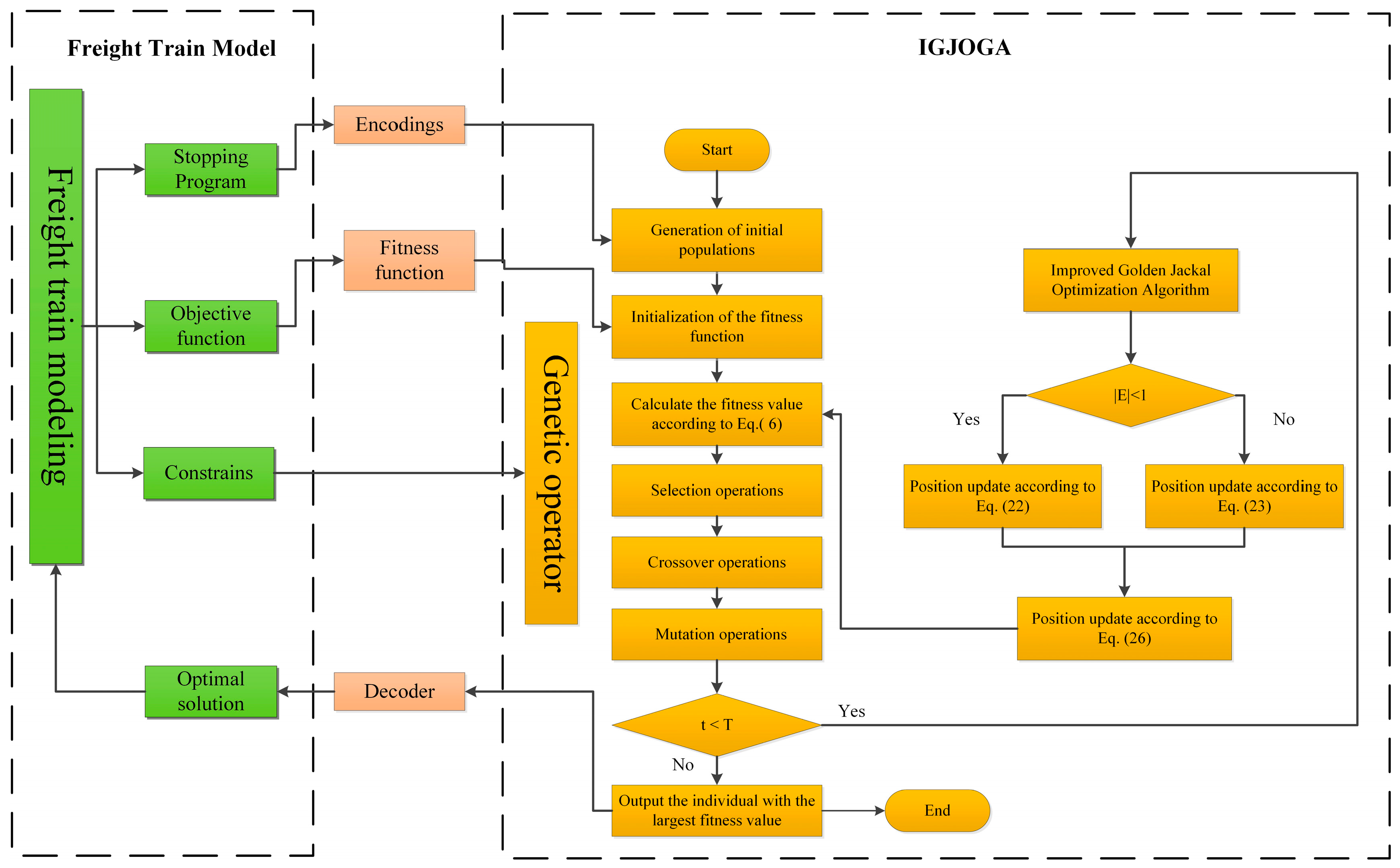
The flowchart of the IGJOGA is shown in Figure 3.

5. Simulation Experiment and Result Analysis

5.1. CEC2022 Test Function

To evaluate the performance of the improved algorithm, we compare the original GJO, the proposed IGJOGA, a baseline GA, and SCSO [24] on the CEC 2022 benchmark functions; see [25] for details of the suite.
All experiments were conducted on a machine equipped with an 11th-generation Intel Core i9-11900K (3.50 GHz) and 32 GB RAM, running Windows 10, with MATLAB R2021b as the simulation environment. Algorithm parameters are listed in Table 1. For all algorithms, we set the initial population size to N = 50 , the maximum number of iterations to T = 500 , and the problem dimension to D I M = 10 . Each configuration was executed for 30 independent runs, and we report the mean, best, worst, and variance of the objective values. Table 2 summarizes the CEC 2022 benchmark functions.
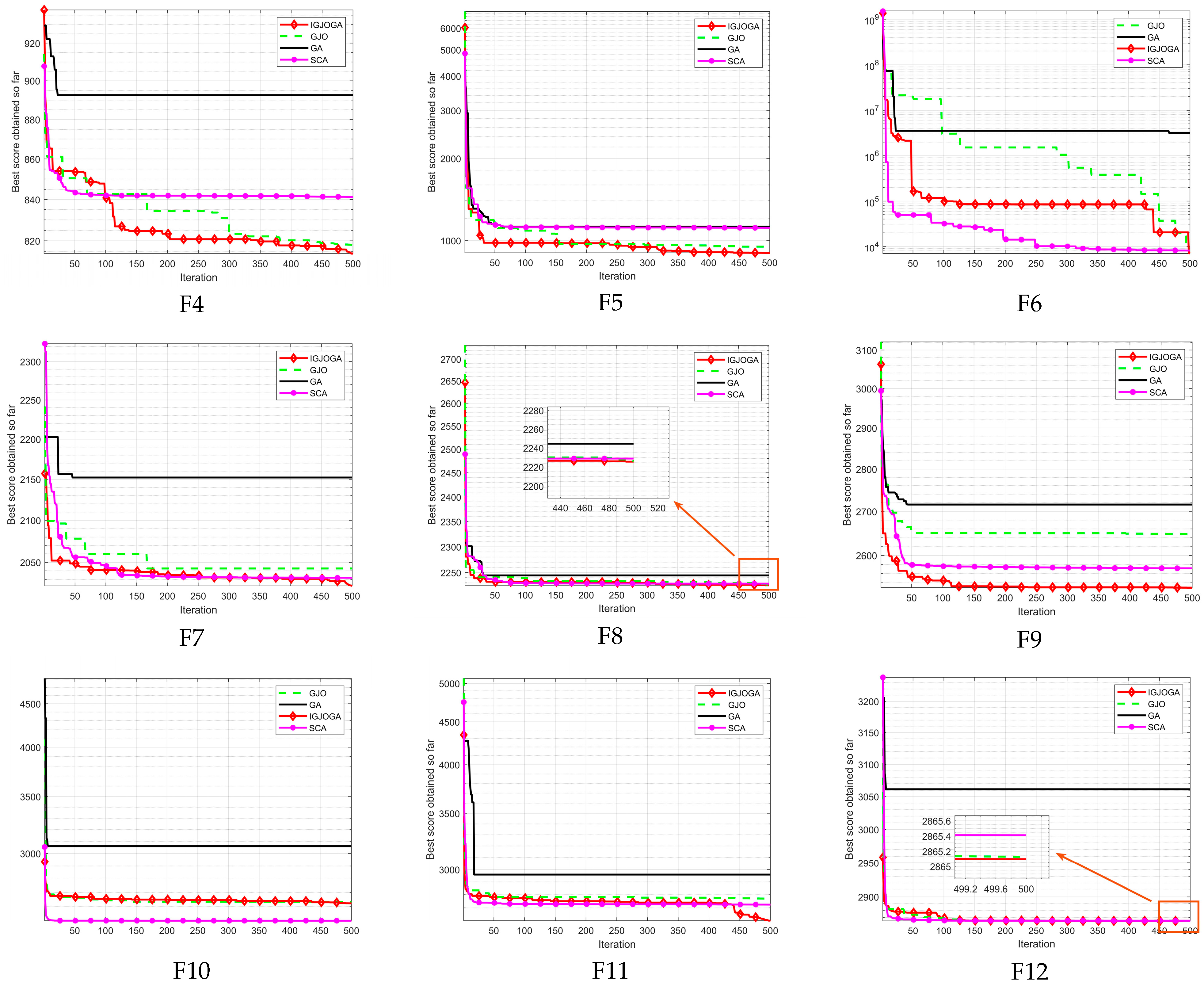
Table 3 presents the test results of the four algorithms, while Figure 4 displays the convergence curves of these algorithms in the CEC2022 test function.
It can be seen from Table 3 that IGJOGA reaches the theoretical optimum on F3. On F1 and F2, it attains values closest to the theoretical optimum among the three algorithms. Although a poor worst-case outcome inflates the mean over 30 independent runs, IGJOGA’s average remains the closest to the theoretical optimum. For F4, F7, F8, and F11, IGJOGA does not reach the theoretical optimum, yet its mean performance is still the best (smallest) among the three algorithms. On F5, F8, F9, and F12, the improved algorithm’s average is closer to the theoretical optimum than that of the competing methods. This demonstrates the effectiveness of the proposed adaptive weighting strategy: smaller weights are applied in early iterations to promote global exploration, while larger weights are used in later iterations to improve solution accuracy by strengthening local search (exploitation).
However, IGJOGA requires more time to reach the optimum. This indicates that the method enhances search performance at the expense of time efficiency; nevertheless, the additional runtime is acceptable given the quality of the final solution. Consequently, IGJOGA holds a clear search advantage over other algorithms.
As shown in Figure 4, the performance gap between the improved and original algorithms on F5, F8, F9, F10, and F11 is modest. Even so, the improved method can still escape local optima, likely due to the t-distribution–based variation strategy. Overall, the improved algorithm demonstrates advantages over the original and delivers better performance.

5.2. Wilcoxon Rank Sum Test

The Wilcoxon rank-sum test [26] is a non-parametric method. Table 3 reports the mean, best, worst, and standard deviation for three algorithms on the CEC 2022 benchmark suite. Because these summary statistics alone do not provide a rigorous significance assessment, we further apply the Wilcoxon rank-sum test. Table 4 presents the p-values comparing IGJOGA with each of the other two algorithms over 30 independent runs. Using a 5% significance level (p < 0.05), all reported p-values in Table 4 are below 0.05, indicating that the proposed IGJOGA algorithm is statistically superior to the competing methods on the CEC 2022 benchmarks.

5.3. Time Complexity Analysis

The time complexity depends on the population size ( N ) of the algorithm, the problem dimension ( D ), and the number of iterations ( T ).
For the original GJO algorithm:
During the initialization phase, the computational cost of the algorithm is O ( N × D ) . At this stage, the GJO algorithm generates random golden jackals in the problem space.
During the fitness evaluation phase for each individual, the complexity is O ( T × D ) . At this point, the GJO algorithm obtains the corresponding fitness values.
During the position update phase, the algorithm’s complexity is O ( T × N × D ) . When N = D , the GJO algorithm’s complexity is O ( G J O ) = O ( N × D ) + O ( T × D ) + O ( T × N × D ) .
For the GA algorithm:
During the initialization phase, the computational complexity of the algorithm is O ( N × D ) .
The computational complexity required to compute N chromosomes is O ( N ) ; The computational complexity for calculating the selection probability of each individual during the selection operation is O ( N ) ; the computational complexity for performing pairwise cross-over on the population during the cross-over operation is O ( N × D ) ; the computational complexity for performing mutation checks on each chromosome during the mutation operation is O ( N × D ) . Therefore, the overall computational complexity of the GA is O ( G A ) = 2 × O ( N ) + 3 × O ( N × D ) .
For the IGJOGA algorithm:
Although an adaptive weighting strategy has been introduced, no additional operations have been added, so the algorithm complexity for this stage remains O ( T × D ) ; in the position update stage, a t-distribution mutation strategy has been introduced, resulting in an algorithm complexity of O ( 2 × T × N × D ) . Additionally, the GA algorithm is integrated, resulting in an improved algorithm complexity of O ( I G J O G A ) = O ( T × D ) + O ( 2 × T × N × D ) + 2 × O ( N ) + 3 × O ( N × D ) . The improved time complexity is higher than the original time complexity, so the computation time for solving problems is longer compared to other algorithms.

5.4. Example Simulation

To further validate the algorithm’s effectiveness, we conduct an optimization experiment on the train departure schedule for a five-city network comprising Chengdu, Guiyang, Chongqing, Xi’an, and Kunming. The experiment runs for 50 iterations with a population size of 80. Station nodes are denoted by the letters a–e, as listed in Table 5.
A binary encoding scheme was developed for a five-city freight-train timetable. The corridor between each pair of stations is divided into ten segments, and each segment is further split into upbound and downbound directions, yielding a total of 20 departure-frequency variables. Trains operate unidirectionally, and the station-level departure frequencies are reported in Table 6.
It is assumed that there are three intermediate stations between the origin (O) and destination (D), and each intermediate station is assigned an opening frequency for a specific stopping scheme. Consequently, the chromosome length in the genetic algorithms is 20 × ( 3 + 3 ) × 8 = 960 . The stopping schemes for the intermediate stations are listed in Table 7, where 0 denotes no stop and 1 denotes a stop.
The distance between the origin (O) and destination (D) is shown in Table 8. Checking the related information, the predicted value of freight transportation for high-value-added goods between each city node is shown in Table 9 [4].
The relevant parameters involved in this paper were solved using MATLAB 2021b. The values of each variable are as follows: the average revenue per kilometer of operation is C 1 = 0.406   ( yuan / kg km ) ; the direct cost per kilometer is C 2 = 0.11   ( yuan / kg km ) ; and the profile cost is C 3 = 100   ( yuan / trip ) . The average loading capacity of each car in the freight train is q = 7.55   ( tons / car ) , the number of groupings of each train is eight, so the maximum carrying capacity of each freight train is 7.55 × 8 = 60.4   ( tons / train ) .
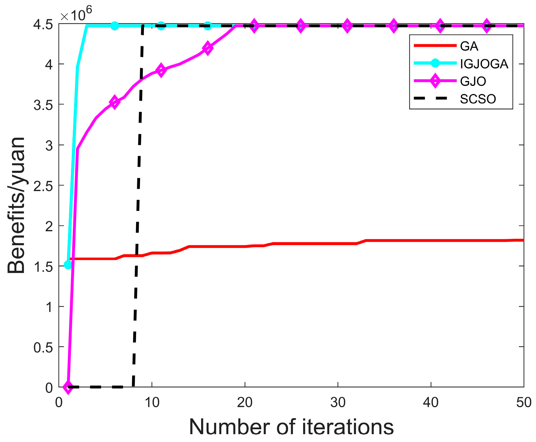
The IGJOGA algorithm attains an objective value of Z = 4 , 471 , 290 yuan, the GJO algorithm achieves the same value of Z = 4 , 471 , 290 yuan, and the GA algorithm yields Z = 2 , 341 , 480 yuan. The identical outcomes for GJO and IGJOGA confirm their consistency. The resulting train operation schedules are reported in Table A1 and Table A2 (Appendix A). The enterprise benefits obtained by IGJOGA are summarized in Table A3 (Appendix A), and the benefit curves for all three algorithms are shown in Figure 5.
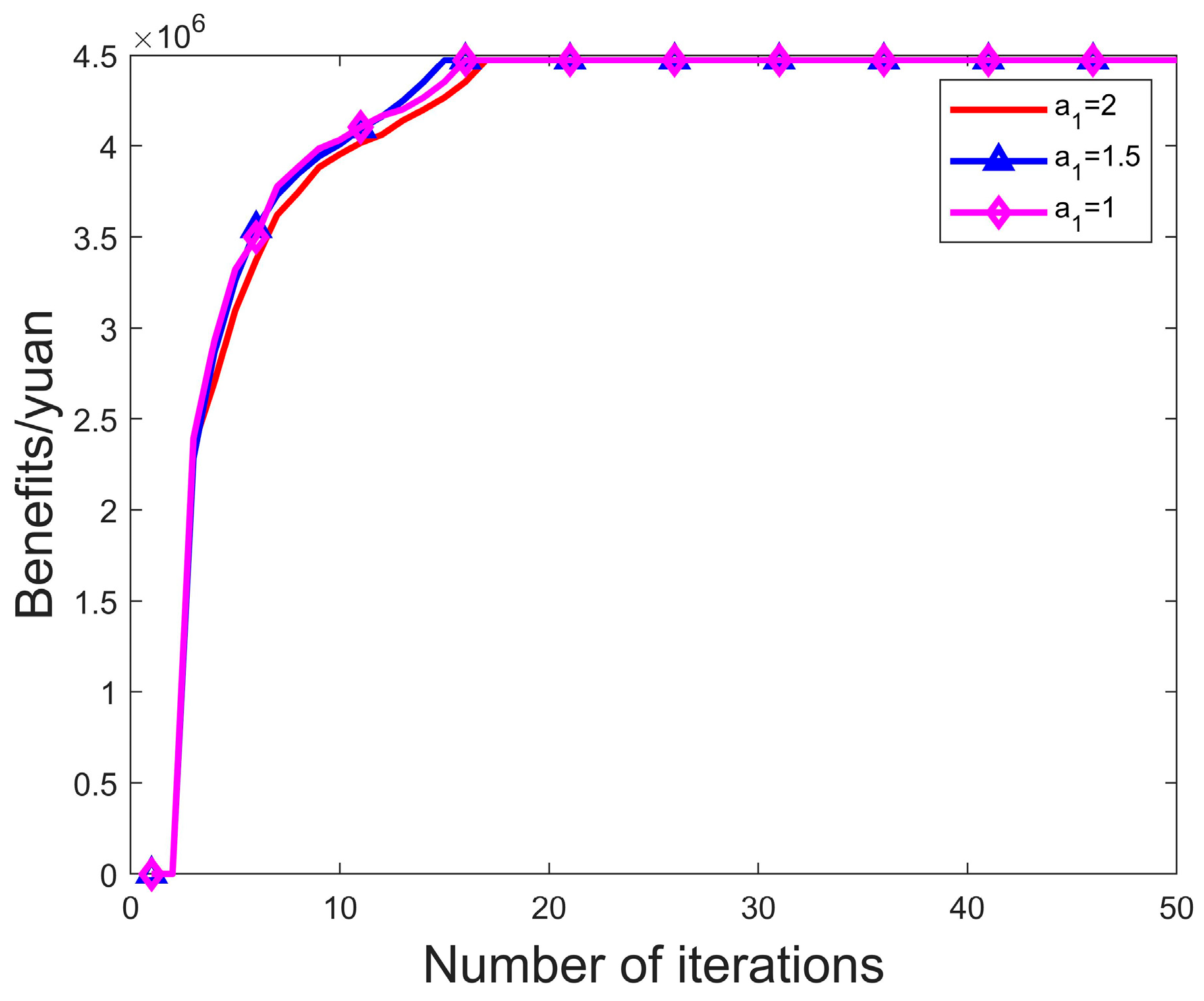
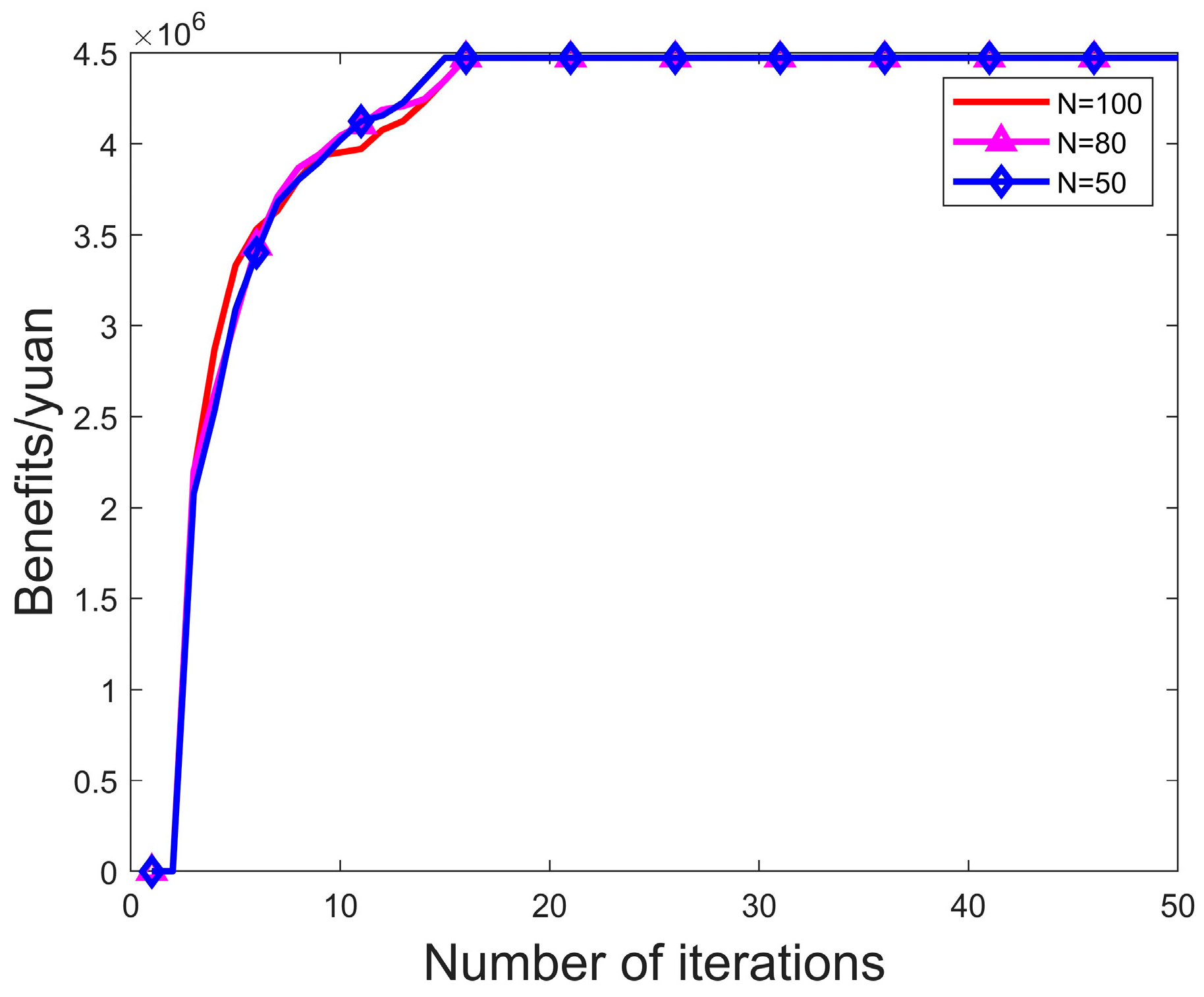
To assess parameter sensitivity, we examine the impact of key hyperparameters. The proposed IGJOGA employs three: population size N , parameter a 1 , and the maximum iteration count. Because the maximum iteration count was fixed at 100 and all algorithms reached the optimum within 20 generations, we do not analyze the effect of the iteration limit. The influences of N and a 1 on performance are illustrated in Figure 6 and Figure 7.
From Figure 5, IGJOGA is seen to reach the model’s optimal objective value much faster, aligning with the goal of maximizing freight-train operational efficiency. Both GJO and IGJOGA achieve the same optimum, indicating that incorporating advanced metaheuristics can accelerate the solution process without compromising solution quality. Specifically, GJO attains the optimum at the 22nd generation, whereas IGJOGA does so by the 4th generation, demonstrating that integrating IGJO mechanisms into GA markedly enhances its search capability. As shown in Figure 6 and Figure 7, the impact of parameter changes on experimental results is evident. When a1 is 1.5, the optimal value is found in the fifteenth iteration; when a1 is 1 or 2, the optimal value is found in the sixteenth iteration. Additionally, when a1 is 1.5, the time taken is 22.13 s, while when a1 is 1 or 2, the times taken are 24.33 s and 24.65 s, respectively. This also indicates that the algorithm is most efficient when a1 is 1.5. When N is 50, the optimal value is found in the fifteenth iteration; when N is 80 or 100, the optimal value is found in the sixteenth iteration. Therefore, setting N to 50 and a1 to 1.5 improves the algorithm’s search performance. The model’s results for IGJOGA and GA are reported in Table A1 and Table A2. The outcomes produced by GJO are consistent with those of IGJOGA.
As shown in Table A1 and Table A2, the freight-train demand across the five city nodes computed by IGJOGA is 364 trains, compared with 181 trains obtained by GA. These results indicate that the improved optimization algorithm more effectively maximizes enterprise benefits and satisfies the specified objective function.

6. Conclusions

Driven by China’s rapid economic growth and ongoing rail freight reforms, the express logistics sector has expanded swiftly. The rail freight industry now prioritizes safety, reliability, convenience, and efficiency. High-value goods impose stringent requirements on timeliness, security, and cost-effectiveness—requirements that traditional freight train models do not adequately satisfy.
This paper addresses the optimization of freight train operation schemes in light of current rail freight conditions and demand characteristics. Based on the present development of rail freight and an analysis of freight demand in five major Chinese cities, we design a new freight train operation scheme. The specific work is as follows:
(1)
We formulate a multi-objective freight train operation planning model that maximizes enterprise operational efficiency and the number of runs, minimizes intermediate stops, and explicitly accounts for train operating costs.
(2)
To solve the model, we propose an Improved Golden Jackal Optimizer–based Genetic Algorithm (IGJOGA), which effectively addresses the premature convergence and low efficiency of standard GA, thereby improving solution quality and convergence speed for this problem.
(3)
We study freight rail segments among five major Chinese cities, compile node-level data, and apply IGJOGA to the proposed model. Experimental results show that the algorithm identifies a maximum freight train benefit of 4,471,294 yuan, and the accommodated train demand increases by 50.27% compared with the GA baseline.
(4)
Compared with other state-of-the-art optimization algorithms, the proposed method is better suited to freight train operation planning and solves the model more efficiently.
The railway network is a complex, large-scale system shaped by numerous interacting factors. Although the freight train operation optimization scheme proposed in this paper achieves the goal of maximizing enterprise benefits, several issues remain that warrant further investigation:
(1)
It is necessary to further analyze the operation organization of freight train services, considering not only individual train conditions but also comprehensive passenger and freight scenarios;
(2)
The model assumes a constant operating speed and does not examine train performance under varying speeds or alternative speed profiles;
(3)
The study relies solely on numerical simulations and has not yet been validated in real-world operational settings.

Author Contributions

Conceptualization, Y.Y. and J.Z.; methodology, Z.Y.; software, Y.J.; validation, Y.Y., J.Z., and Z.Y.; formal analysis, Y.Y.; investigation, Y.J.; resources, Y.Y.; data curation, J.Z.; writing—original draft preparation, Y.Y.; writing—review and editing, J.Z.; visualization, Y.Y.; supervision, Y.Y.; project administration, Y.Y.; funding acquisition, Y.Y. All authors have read and agreed to the published version of the manuscript.

Funding

This work was supported by Key Projects of National Energy Investment Group Co., Ltd. (BZ2023-033YS).

Institutional Review Board Statement

Not applicable.

Informed Consent Statement

Not applicable.

Data Availability Statement

The data that support the results of this study are available from the corresponding author upon reasonable request.

Conflicts of Interest

The authors declare that the research was conducted in the absence of any commercial or financial relationships that could be construed as a potential conflict of interest.

Appendix A

Table A1. IGJOGA algorithm for solving freight train frequency.
ODNumber of Train Tripsi-jFrequency
ba1 7
ab1 7
ca1 7
ac1 7
da1 7
ad1 7
ea1 7
ae1 7
bc1 7
cb1 7
db1 7
bd1 7
eb1 7
be1 7
dc1 7
cd1 7
ec1 7
ce1 7
ed1 7
de1 7
ca1b 7
ac1b 7
da1b 7
ad1b 7
ea1b 7
ae1b 7
da1c 7
ad1c 7
ea1c 7
ae1c 7
ea1d 7
ae1d 7
db1c 7
bd1c 7
eb1c 7
be1c 7
eb1d 7
be1d 7
ec1d 7
ce1d 7
da1cb 7
ad1bc 7
ea1cb 7
ae1bc 7
ea1db 7
ae1bd 7
ea1dc 7
ae1cd 7
eb1dc 7
be1cd 7
ea1dcb7
ae1bcd7
Table A2. GA algorithm for solving freight train frequency.
ODNumber of Train Tripsi-jFrequency
ab1 5
ca1 6
ac1 6
da1 7
ad1 6
ea1 7
ae1 4
bc1 1
db1 3
eb1 3
be1 1
dc1 4
ce1 1
ca1b 5
da1b 4
ad1b 7
ea1b 3
ae1b 4
da1c 5
ad1c 4
ea1c 1
ae1c 1
ea1d 6
ae1d 7
bd1c 7
eb1c 7
be1c 7
eb1d 3
be1d 6
ec1d 6
ad1bc 4
ea1cb 7
ae1bc 7
ea1db 7
ea1dc 5
ae1cd 7
be1cd 6
ea1dcb1
Table A3. Optimized business benefits.
Transportation Revenue/YuanDirect Cost/YuanIndirect Cost/YuanEnterprise Efficiency/Yuan
4,536,89419,60046,0004,471,294

References

  1. Wang, B.; He, S. Resource planning optimization model and algorithm for multi-modal express shipment network. Tiedao Xuebao/J. China Railw. Soc. 2017, 39, 10–16. [Google Scholar]
  2. Chang, Y.; Lei, S.; Teng, J.; Zhang, J.; Zhang, L.; Xu, X. The energy use and environmental emissions of high-speed rail transportation in China: A bottom-up modeling. Energy 2019, 182, 1193–1201. [Google Scholar] [CrossRef]
  3. Yu, X.; Zhou, L.; Huo, M.; Yu, X. Research on High-Speed Railway Freight Train Organization Method considering Different Transportation Product Demands. Math. Probl. Eng. 2021, 2021, 5520867. [Google Scholar] [CrossRef]
  4. Xiao, H.; Huang, S.; Hang, B.; Zhang, Q. Optimization of operation scheme for express freight railway. Kuwait J. Sci. 2021, 48, 50–58. [Google Scholar] [CrossRef]
  5. Archetti, C.; Peirano, L.; Speranza, M.G. Optimization in multimodal freight transportation problems: A survey. Eur. J. Oper. Res. 2022, 299, 1–20. [Google Scholar] [CrossRef]
  6. Hosseini, S.; Al Khaled, A. Freight flow optimization to evaluate the criticality of intermodal surface transportation system infrastructures. Comput. Ind. Eng. 2021, 159, 107522. [Google Scholar] [CrossRef]
  7. Smolyanivov, A.; Yushkova, S.; Sirina, N. Transport infrastructure condition for organizing piggyback traffic. IOP Conf. Ser. Earth Environ. Sci. 2019, 403, 012200. [Google Scholar] [CrossRef]
  8. Taslimi, B.; Sarijaloo, F.B.; Liu, H.; Pardalos, P.M. A novel mixed integer programming model for freight train travel time estimation. Eur. J. Oper. Res. 2022, 300, 676–688. [Google Scholar] [CrossRef]
  9. Pineda-Jaramillo, J.; Viti, F. Identifying the rail operating features associated to intermodal freight rail operation delays. Transp. Res. Part C Emerg. Technol. 2023, 147, 103993. [Google Scholar] [CrossRef]
  10. Li, S.; Lv, H.; Xu, C.; Chen, T.; Zou, C. Optimized train path selection method for daily freight train scheduling. IEEE Access 2020, 8, 40777–40790. [Google Scholar] [CrossRef]
  11. Wang, Z.; Ceder, A. Efficient design of freight train operation with double-hump yards. J. Oper. Res. Soc. 2017, 68, 1600–1619. [Google Scholar] [CrossRef]
  12. Holland, J.H. Genetic algorithms. Sci. Am. 1992, 267, 66–73. [Google Scholar] [CrossRef]
  13. Sohail, A. Genetic algorithms in the fields of artificial intelligence and data sciences. Ann. Data Sci. 2023, 10, 1007–1018. [Google Scholar] [CrossRef]
  14. Pehlivanoglu, Y.V.; Pehlivanoglu, P. An enhanced genetic algorithm for path planning of autonomous UAV in target coverage problems. Appl. Soft Comput. 2021, 112, 107796. [Google Scholar] [CrossRef]
  15. Zhu, Z.; Liu, Y.; He, Y.; Wu, W.; Wang, H.; Huang, C.; Ye, B. Fuzzy PID control of the three-degree-of-freedom parallel mechanism based on genetic algorithm. Appl. Sci. 2022, 12, 11128. [Google Scholar] [CrossRef]
  16. Jia, X.; He, R.; Chai, H. Optimizing the number of express freight trains on a high-speed railway corridor by the departure period. IEEE Access 2020, 8, 100058–100072. [Google Scholar] [CrossRef]
  17. Li, S.; Lang, M.; Li, S.; Chen, X.; Yu, X.; Geng, Y. Optimization of high-speed railway line planning with passenger and freight transport coordination. IEEE Access 2022, 10, 110217–110247. [Google Scholar] [CrossRef]
  18. Li, H.; Tian, C.; Zhang, S.; Jiang, Y. Calculation method for carrying capacity of mixed passenger and freight railway based on improved rotor model. China Railw. Sci. 2021, 42, 144–155. [Google Scholar]
  19. Hu, W.; Dong, J.; Hwang, B.G.; Ren, R.; Chen, Z. Is mass rapid transit applicable for deep integration of freight-passenger transport? A multi-perspective analysis from urban China. Transp. Res. Part A Policy Pract. 2022, 165, 490–510. [Google Scholar] [CrossRef]
  20. Milenković, M.; Bojović, N.; Abramin, D. Railway freight wagon fleet size optimization: A real-world application. J. Rail Transp. Plan. Manag. 2023, 26, 100373. [Google Scholar] [CrossRef]
  21. Katoch, S.; Chauhan, S.S.; Kumar, V. A review on genetic algorithm: Past, present, and future. Multimed. Tools Appl. 2021, 80, 8091–8126. [Google Scholar] [CrossRef] [PubMed]
  22. Chopra, N.; Ansari, M.M. Golden jackal optimization: A novel nature-inspired optimizer for engineering applications. Expert Syst. Appl. 2022, 198, 116924. [Google Scholar] [CrossRef]
  23. Lou, T.s.; Yue, Z.P.; Jiao, Y.Z.; He, Z.D. A hybrid strategy-based gjo algorithm for robot path planning. Expert Syst. Appl. 2024, 238, 121975. [Google Scholar] [CrossRef]
  24. Seyyedabbasi, A.; Kiani, F. Sand Cat swarm optimization: A nature-inspired algorithm to solve global optimization problems. Eng. Comput. 2023, 39, 2627–2651. [Google Scholar] [CrossRef]
  25. Yazdani, D.; Branke, J.; Omidvar, M.N.; Li, X.; Li, C.; Mavrovouniotis, M.; Nguyen, T.T.; Yang, S.; Yao, X. IEEE CEC 2022 competition on dynamic optimization problems generated by generalized moving peaks benchmark. arXiv 2021, arXiv:2106.06174. [Google Scholar]
  26. Derrac, J.; García, S.; Molina, D.; Herrera, F. A practical tutorial on the use of non-parametric statistical tests as a methodology for comparing evolutionary and swarm intelligence algorithms. Swarm Evol. Comput. 2011, 1, 3–18. [Google Scholar] [CrossRef]
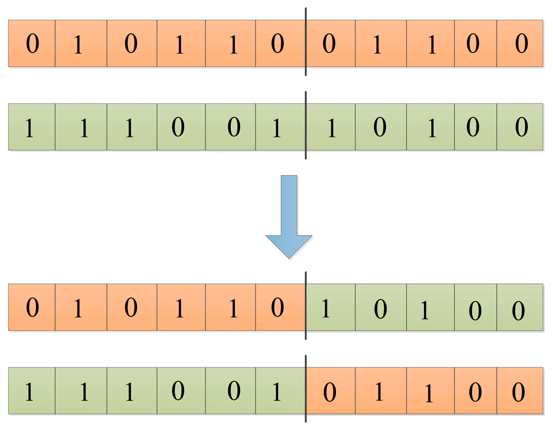
Figure 1. Cross-over operation.
Applsci 15 09326 g001
Figure 2. Mutation operation.
Applsci 15 09326 g002
Figure 3. Flowchart of the IGJOGA algorithm.
Applsci 15 09326 g003
Figure 4. Convergence curves of the three algorithms.
Applsci 15 09326 g004aApplsci 15 09326 g004b
Figure 5. Convergence curve of enterprise benefits.
Applsci 15 09326 g005
Figure 6. Effect of parameter C1 variation on the experiment.
Applsci 15 09326 g006
Figure 7. Effect of parameter N formation on the experiment.
Applsci 15 09326 g007
Table 1. Parameter settings for each algorithm.
AlgorithmParameters Value
IGJOGAω1 = 0.9
ω2 = 0.2
α = 1.5
Mutation probability pm = 0.001
Cross-over probability pc = 0.6
E1 linearly decreases from 1.5 to 0
GJO
GA
E1 linearly decreases from 1.5 to 0
Mutation probability pm = 0.001
Cross-over probability pc = 0.6
Table 2. CEC2022 test function.
NameNo.FunctionFmin
Unimodal FunctionF1Shifted and full Rotated Zakharov Function300
Basic FunctionsF2Shifted and full Rotated Rosenbrock’s Function400
F3Shifted and full Rotated Expanded Schaffer’s f6 Function600
F4Shifted and full Rotated Non-Continuous Rastrigin’s Function800
F5Shifted and full Rotated Lévy Function900
Hybrid FunctionsF6Hybrid Function 1 (N = 3)1800
F7Hybrid Function 2 (N = 6)2000
F8Hybrid Function 3 (N = 5)2200
Composition FunctionsF9Composition Function 1 (N = 5)2300
F10Composition Function 2 (N = 4)2400
F11Composition Function 3 (N = 5)2600
F12Composition Function 4 (N = 6)2700
Search Range: [−100, 100]Dim
Table 3. Test results of the three algorithms.
FunctionIndicatorsIGJOGAGJOGASCSO
F1Best3.11 × 1023.99 × 1027.98 × 1033.27 × 102
Mean4.60 × 1022.82 × 1033.29 × 1042.00 × 103
Std2.00 × 1022.34 × 1031.38 × 1041.67 × 103
Worst1.46 × 1031.02 × 1046.19 × 1047.42 × 103
Time6.92270.263770.211380.70663
F2Best4.00 × 1024.08 × 1024.42 × 1024.00 × 102
Mean4.23 × 1024.41 × 1025.07 × 1024.37 × 102
Std2.73 × 1012.88 × 1014.56 × 1012.98 × 101
Worst4.94 × 1025.23 × 1026.56 × 1024.87 × 102
Time8.07090.295070.22770.75643
F3Best6.00 × 1026.00 × 1026.26 × 1026.01 × 102
Mean6.03 × 1026.07 × 1026.51 × 1026.15 × 102
Std3.10 × 1005.19 × 1001.18 × 1019.15 × 100
Worst6.13 × 1026.18 × 1026.75 × 1026.45 × 102
Time7.41480.362610.365670.80324
F4Best8.08 × 1028.08 × 1028.32 × 1028.14 × 102
Mean8.19 × 1028.26 × 1028.55 × 1028.30 × 102
Std7.88 × 1001.04 × 1011.18 × 1016.74 × 100
Worst8.38 × 1028.48 × 1028.76 × 1028.44 × 102
Time7.81140.290370.239890.75898
F5Best9.00 × 1029.01 × 1029.15 × 1029.04 × 102
Mean9.51 × 1029.90 × 1021.03 × 1031.05 × 103
Std7.65 × 1018.09 × 1011.42 × 1021.44 × 102
Worst1.26 × 1031.19 × 1031.47 × 1031.49 × 103
Time7.46650.30680.253440.75544
F6Best3.00 × 1033.75 × 1031.91 × 1031.92 × 103
Mean8.14 × 1039.56 × 1038.70 × 1033.94 × 103
Std2.51 × 1032.66 × 1032.02 × 1042.04 × 103
Worst1.32 × 1041.82 × 1041.14 × 1058.09 × 103
Time7.34990.287670.228110.74148
F7Best2.01 × 1032.02 × 1032.05 × 1032.02 × 103
Mean2.03 × 1032.05 × 1032.09 × 1032.05 × 103
Std7.71 × 1002.10 × 1013.52 × 1012.59 × 101
Worst2.04 × 1032.10 × 1032.20 × 1032.12 × 103
Time7.49440.432970.325410.80438
F8Best2.20 × 1032.20 × 1032.23 × 1032.22 × 103
Mean2.22 × 1032.23 × 1032.26 × 1032.23 × 103
Std5.52 × 1005.55 × 1004.43 × 1014.04 × 100
Worst2.23 × 1032.24 × 1032.37 × 1032.24 × 103
Time7.66490.39920.344410.83762
F9Best2.53 × 1032.53 × 1032.63 × 1032.53 × 103
Mean2.54 × 1032.58 × 1032.70 × 1032.57 × 103
Std1.98 × 1013.97 × 1014.82 × 1013.78 × 101
Worst2.59 × 1032.68 × 1032.81 × 1032.68 × 103
Time7.61240.361730.300120.82552
F10Best2.50 × 1032.50 × 1032.50 × 1032.50 × 103
Mean2.56 × 1032.56 × 1032.64 × 1032.54 × 103
Std5.87 × 1016.23 × 1012.80 × 1025.98 × 101
Worst2.63 × 1032.64 × 1034.07 × 1032.65 × 103
Time7.43460.339920.288290.79674
F11Best2.60 × 1032.61 × 1032.77 × 1032.60 × 103
Mean2.75 × 1032.87 × 1033.14 × 1032.78 × 103
Std2.11 × 1022.04 × 1023.34 × 1021.80 × 102
Worst3.23 × 1033.25 × 1033.96 × 1033.24 × 103
Time7.55890.386650.33080.83284
F12Best2.86 × 1032.86 × 1032.92 × 1032.86 × 103
Mean2.86 × 1032.87 × 1033.01 × 1032.87 × 103
Std2.58 × 1001.50 × 1014.25 × 1011.56 × 101
Worst2.87 × 1032.93 × 1033.09 × 1032.95 × 103
Time8.2570.391030.33120.84761
Table 4. Experimental results of the Wilcoxon rank sum test on CEC2022.
FunctionDimIGJOGA vs. GJOIGJOGA vs. GAIGJOGA vs. SCSO
F1107.39 × 10−113.02 × 10−117.60 × 10⁻⁷
F2103.34 × 10−35.53 × 10−89.07 × 10−3
F3102.88 × 10−63.02 × 10−111.01 × 10⁻⁸
F4109.07 × 10−34.50 × 10−112.77 × 10⁻⁵
F5109.88 × 10−31.37 × 10−32.39 × 10−8
F6101.49 × 10−43.77 × 10−42.03 × 10−7
F7101.03 × 10−63.02 × 10−112.77 × 10⁻⁵
F8103.37 × 10−54.08 × 10−115.56 × 10⁻⁴
F9103.47 × 10−103.02 × 10−119.88 × 10⁻³
F10105.83 × 10−36.53 × 10−87.96 × 10−1
F11101.64 × 10−51.07 × 10−91.54 × 10−1
F12101.60 × 10−33.02 × 10−113.64 × 10⁻²
Table 5. Symbolic representation of cities.
Place NameChengduGuiyangChongqingXi’anKunming
symbolabcde
Table 6. Frequency of departures between the five stations.
Upward DirectionDownward Directions
NO.ODOD
1abba
2acca
3adda
4aeea
5bccb
6bddb
7beeb
8cddc
9ceec
10deed
Table 7. Stopping options from the origin to the destination.
Midway Station 1Midway Station 2Midway Station 3
000
001
010
011
100
101
110
111
Table 8. Distance between cities (Km).
Oabcde
D
a0157533688996
b1570376531839
c5333760155463
d6885311550308
e9968394633080
Table 9. Inter-city shipments of high-value-added commodities (trains/day).
Oabcde
D
a059.14259106.120485.5469580.18532
b142.2271085.6330669.0314464.70492
c133.456344.78157064.7744260.7147
d196.587765.9655118.3629089.4358
e188.343763.19919113.399391.414630
Disclaimer/Publisher’s Note: The statements, opinions and data contained in all publications are solely those of the individual author(s) and contributor(s) and not of MDPI and/or the editor(s). MDPI and/or the editor(s) disclaim responsibility for any injury to people or property resulting from any ideas, methods, instructions or products referred to in the content.