Detection of Lead Contamination Using Bioelectrical Signals of Aloe vera var. Chinensis: A Wavelet-Based and Explainable Machine Learning Approach

Abstract

Heavy metal contamination, particularly lead (Pb), represents a threat to ecosystems and human health. This study investigates the variety Aloe vera var. Chinensis as a plant sensing platform for detecting the presence of lead by characterizing its bioelectrical response. A low-cost system based on Arduino was developed to acquire real-time electrical signals from 160 plants, equally divided between two groups: control conditions (n = 80) and Pb acetate exposure (500 mg/L; n = 80). Two recording sessions per plant were obtained after the plant had stabilized, resulting in 320 labeled measurements. The signals were characterized using the discrete wavelet transform (DWT), autoregressive (AR) models, and complexity measures based on entropy. Three classifiers—Support Vector Machine, Random Forest, and XGBoost—were trained and evaluated using five-fold cross-validation and a held-out test set with plant disjoint samples. XGBoost achieved the highest performance (accuracy = 93.0%; precision = 92.5%; recall = 93.8%; F1-score = 93.1%; and 95% CI for accuracy: 90.4–95.2% via bootstrap), significantly outperforming the other models. SHAP analysis revealed that midscale wavelet entropy and energy features, along with AR residual variance, were the most discriminative for Pb detection. These findings demonstrate a scalable, low-cost, and interpretable biosensing framework with potential applications in real-time environmental monitoring and early detection of heavy metal contamination.

1. Introduction

Heavy metal contamination, particularly lead (Pb), remains a critical global concern due to its persistence, bioaccumulation, and toxicological impact on ecosystems and human health. In the literature, systematic reviews have quantified Pb levels in multiple environmental media—including soil, dust, water, food, and air—highlighting contamination in both industrialized and developing regions. For instance, Frank et al. [1] analyzed more than two decades of U.S. monitoring data, showing that soil Pb concentrations frequently exceeded the U.S. EPA screening level of 400 mg/kg, with over 30% of samples above safe limits in some regions. Similarly, Oloruntoba et al. [2] documented substantial Pb contamination in Nigeria’s soils, water, and food, with values in agricultural soils up to 20 times higher than the WHO guideline of about 50 mg/kg. The WHO estimates that lead exposure contributes to over 900,000 deaths annually, primarily through cardiovascular and neurological effects [3], and identifies lead as a chemical of major public health concern [3]. Long-term exposure has been associated with cognitive impairment in children and reduced life expectancy in adults [4]. In addition, recent U.S. EPA updates lowered the residential soil screening level for lead from 400 to 200  mg/kg (and to 100 mg/kg where multiple sources are present) [5].

Despite the availability of laboratory-based analytical methods—such as atomic absorption spectroscopy (AAS) and inductively coupled plasma–mass spectrometry (ICP-MS)—these techniques require expensive instrumentation, skilled personnel, and centralized facilities, limiting their deployment in resource-constrained or remote areas. This gap has motivated research into innovative, field-deployable, and low-cost detection strategies capable of providing continuous and non-invasive monitoring. Within this context, plant-based biosensing emerges as a promising avenue, leveraging the physiological responsiveness of species such as Aloe vera to environmental stressors while enabling scalable environmental diagnostics.

Electrical signals in plants are rapid variations in the membrane potential in plant cells, typically generated in response to external stimuli such as environmental stress, injury, or chemical exposure. These signals originate from ionic imbalances and influence critical physiological processes like stomatal regulation, photosynthesis, and water and nutrient uptake [6]. The scientific interest in plant electrophysiology dates back to the work of Burdon-Sanderson in 1873, who observed that applying mechanical stimuli to Dionaea muscipula leaves elicited electrical changes [7]. Later, Chandra Bose advanced the field by developing equipment to measure these signals, establishing that plants exhibit measurable electrical responses to stimuli like light. More recently, Volkov and collaborators examined how Aloe vera responds electrically to thermal stimuli, validating its potential as a model for electrophysiological research [8].

Aloe vera var. Chinensis, known for its environmental resilience and water retention capacity, has become a subject of increasing attention for its potential use as a biosensor. Prior studies, such as that by Shokri (2016), explored Aloe vera as a phytoremediator of heavy metals, suggesting that lead contamination significantly alters its physiology, possibly reflected in its electrical signature [9].

Traditional analysis of plant electrical signals has included tools such as Fourier transforms, wavelet analysis, and autoregressive (AR) modeling [10,11]. These tools enable the extraction of statistical and spectral features, which can be fed into machine learning algorithms to identify or classify specific plant states. For example, Kumar et al. [12] used electrical features to classify ozone exposure, while Yu et al. [13] applied PCA to distinguish mercury contamination in tobacco plants. Given that plant electrical signals are typically low-frequency, nonlinear, and non-stationary [14], it is essential to utilize both non-parametric and parametric approaches for accurate analysis. The discrete wavelet transform (DWT) allows time–frequency localization of transient signal features, while AR models capture temporal dependencies in the signal. These complementary techniques enable a robust characterization of electrical responses under environmental stress.

On the other hand, in the context of artificial intelligence, recent advances in deep learning for time-series modeling, particularly Long Short-Term Memory (LSTM) networks and transformer-based architectures, have demonstrated remarkable capabilities in capturing long-range dependencies and complex temporal dynamics. For example, Yang et al. [15] applied convolutional and recurrent neural networks to predict complex erosion profiles in steam distribution headers, showing that these models can accurately capture intricate temporal patterns in industrial processes. Similarly, Geneva and Zabaras [16] provided a comprehensive review of transformer architectures for modeling physical systems, highlighting their ability to efficiently learn relevant temporal relationships over long sequences. In addition, Zhou et al. [17] proposed the Informer architecture for long-sequence forecasting, and Wu et al. [18] introduced Autoformer, which integrates decomposition and autocorrelation mechanisms for improved prediction accuracy. Although the present study focuses on algorithms with high interpretability and proven performance on small datasets (SVM, RF, and XGBoost), future research could explore these state-of-the-art architectures for enhanced modeling of plant bioelectrical signals, especially in scenarios with larger datasets and extended monitoring periods. In particular, the ability of transformers to capture non-local relationships in temporal sequences could prove valuable for detecting subtle bioelectrical patterns associated with heavy metal-induced stress in plants.

This study presents an integrated methodology that combines the discrete wavelet transform (DWT) and autoregressive (AR) modeling for feature extraction from electrical signals of Aloe vera var. Chinensis, with the objective of classifying the presence or absence of lead (Pb) contamination. This work develops an experiment in a cohort of 160 plants. One group has 80 plants under standard laboratory conditions and another group has 80 subjected to lead acetate (500 mg/L). Bioelectrical signals were acquired using a low-cost Arduino-based system, processed to extract statistical features, and used to train classification algorithms such as Support Vector Machine (SVM), Random Forest, and XGBoost. The expanded dataset enables statistically robust plant disjoint validation and tighter confidence intervals for performance estimates. The results show that XGBoost achieved superior classification performance, supported by SHAP-based feature interpretation. This approach demonstrates the potential of Aloe vera as a biosensor for detecting heavy metal contamination, offering a cost-effective and scalable solution for environmental monitoring applications.

2. Materials and Methods

The methodology used to develop the classification algorithm for detecting the presence of lead in Aloe vera var. Chinensis plants was structured into eight main stages (Figure 1), where protocols and methodologies were followed for the correct recording and processing of biological signals that have enabled other studies to obtain satisfactory results [19,20].

The first stage consisted of establishing the experimental setup, including growth conditions and the controlled lead contamination process, based on procedures similar to those used in prior studies involving plant-based biosensors and phytoremediation systems [8,9].

The second stage focused on acquiring the electrical signals from the Aloe vera plant using a low-cost Arduino-based system, a widely adopted approach in plant electrophysiology due to its accessibility and reliability [21].

In the third stage, signal preprocessing was conducted to remove noise and artifacts, ensuring that the electrical activity matched the known characteristics of plant electrical signals—such as their low amplitude, non-stationary nature, and susceptibility to environmental variations [8,14].

The fourth stage involved non-parametric analysis using signal decomposition techniques such as the discrete wavelet transform (DWT) and Empirical Mode Decomposition (EMD), which are highly effective for analyzing nonlinear and non-stationary biological signals [22]. This allowed for the identification of time–frequency patterns in the electrical response of the plant.

In the fifth stage, a parametric approach was applied through the use of autoregressive (AR) modeling, enabling the characterization of temporal dependencies in the signal [10].

The sixth stage described the extraction of key features from both types of analysis—wavelet-based features such as energy and entropy and AR coefficients with residual error variance—which were used to train machine learning models.

In the seventh stage, classification algorithms were trained to distinguish between contaminated and uncontaminated plants. Finally, in the eighth stage, performance was validated using standard classification metrics and explainability tools such as SHAP values to evaluate model robustness and interpretability [23].

2.1. Experimental Design

Plant: Aloe vera var. Chinensis plants with homogeneous characteristics in size, color, and health status were selected. All specimens were cultivated in a greenhouse in Zacatecas, Mexico, under controlled horticultural practices. The plants had an average height of approximately 40 cm, with leaves measuring between 6 and 8 cm in length and 3 and 4 cm in width, similar to morphometric characteristics reported in prior phytosensing research [8,9].

A total of 160 Aloe vera plants were used, divided into two equal groups: 80 were maintained under controlled, contaminant-free conditions and 80 were exposed to a 500 mg/L aqueous solution of lead acetate to simulate soil contamination, following concentrations aligned with studies of phytotoxic heavy metal exposure [12,13]. From each plant, two independent electrical signal recordings were acquired, resulting in 320 labeled signal instances. The chosen sample size ensured a statistically robust evaluation of classification performance and strengthened the generalizability of the results for this work.

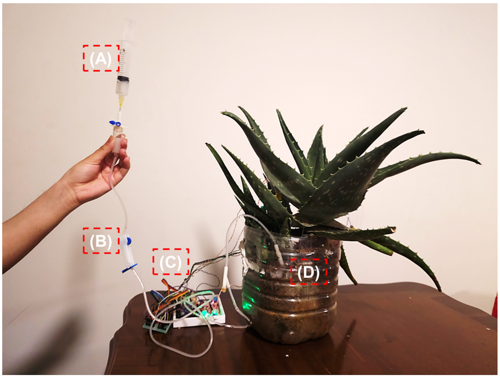
All plants were placed in isolated environments with minimized noise and interference. A simulated photoperiod of 12-h light/dark cycles was implemented using artificial lighting. Measurements were taken in a standardized sequence to reduce potential experimental drift (Figure 2).

To minimize selection bias, plants were randomly assigned to the control and Pb-exposed groups using a random number generator. All specimens were cultivated under identical greenhouse conditions, including potting substrate, photoperiod, irrigation regime, and ambient environment. Measurements were conducted in a standardized sequence to mitigate potential effects of experimental drift. To verify this, the amplitude and key signal features were tested for correlation with chronological measurement order, and no statistically significant associations were observed (p > 0.05), indicating that temporal drift was negligible under the controlled experimental conditions.

Environmental Control Conditions: To control for environmental variables known to influence plant bioelectrical activity, all plants were maintained in a controlled-environment greenhouse during the entire experimental period. Environmental parameters were monitored continuously using integrated sensors in the acquisition system:

• Air temperature: Maintained at 25 ± 1 °C, measured with a DHT11 digital sensor (Aosong Electronics Co., Ltd., Guangzhou, China).
• Relative humidity: Maintained between 55% and 65%, recorded by the DHT11 sensor.
• Light intensity: Maintained at 300–350 µmol·m⁻²·s⁻¹ (photosynthetically active radiation), measured with an LDR photoresistor module calibrated against a PAR meter.
• Soil moisture: Kept between 25% and 30% volumetric water content, measured using an FC-28 capacitive soil moisture sensor (Innovative Technology, Shenzhen, China).

These environmental parameters were selected based on optimal growth conditions for Aloe vera and maintained with minimal variation to prevent confounding effects on bioelectrical responses. No statistically significant differences were detected between control and Pb-exposed groups for any environmental variable. This ensured that observed differences in electrical signals were attributable to Pb exposure rather than uncontrolled environmental fluctuations.

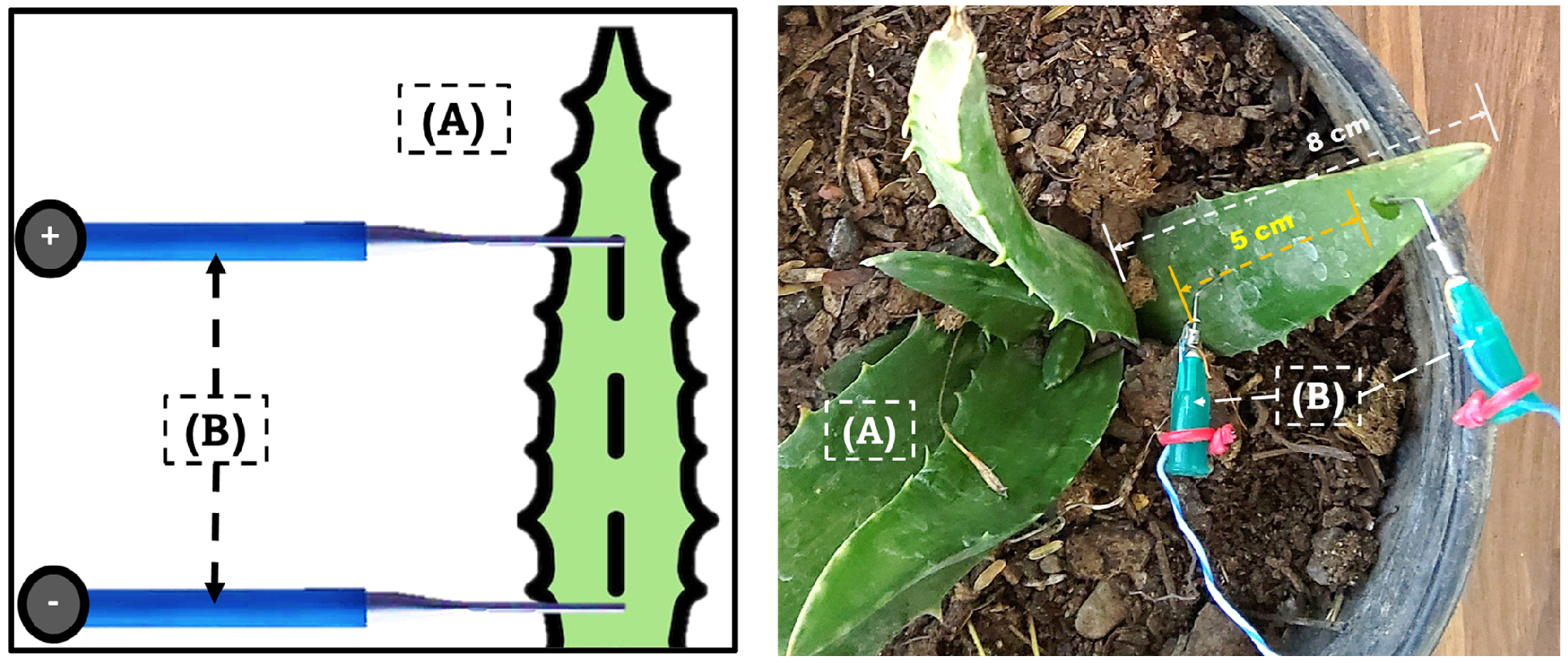
Electrodes: The electrical signal was acquired using the electrode insertion method [10], where two stainless steel acupuncture-grade needles (Hwato, Suzhou Medical Appliance Factory, Suzhou, China) were inserted into the plant tissue at a distance of 5 cm from the stem. One electrode served as the reference (GND) and the other as the active measurement point (Figure 3). This method allows direct access to ionic currents within the plant and has been widely used in plant electrophysiology.

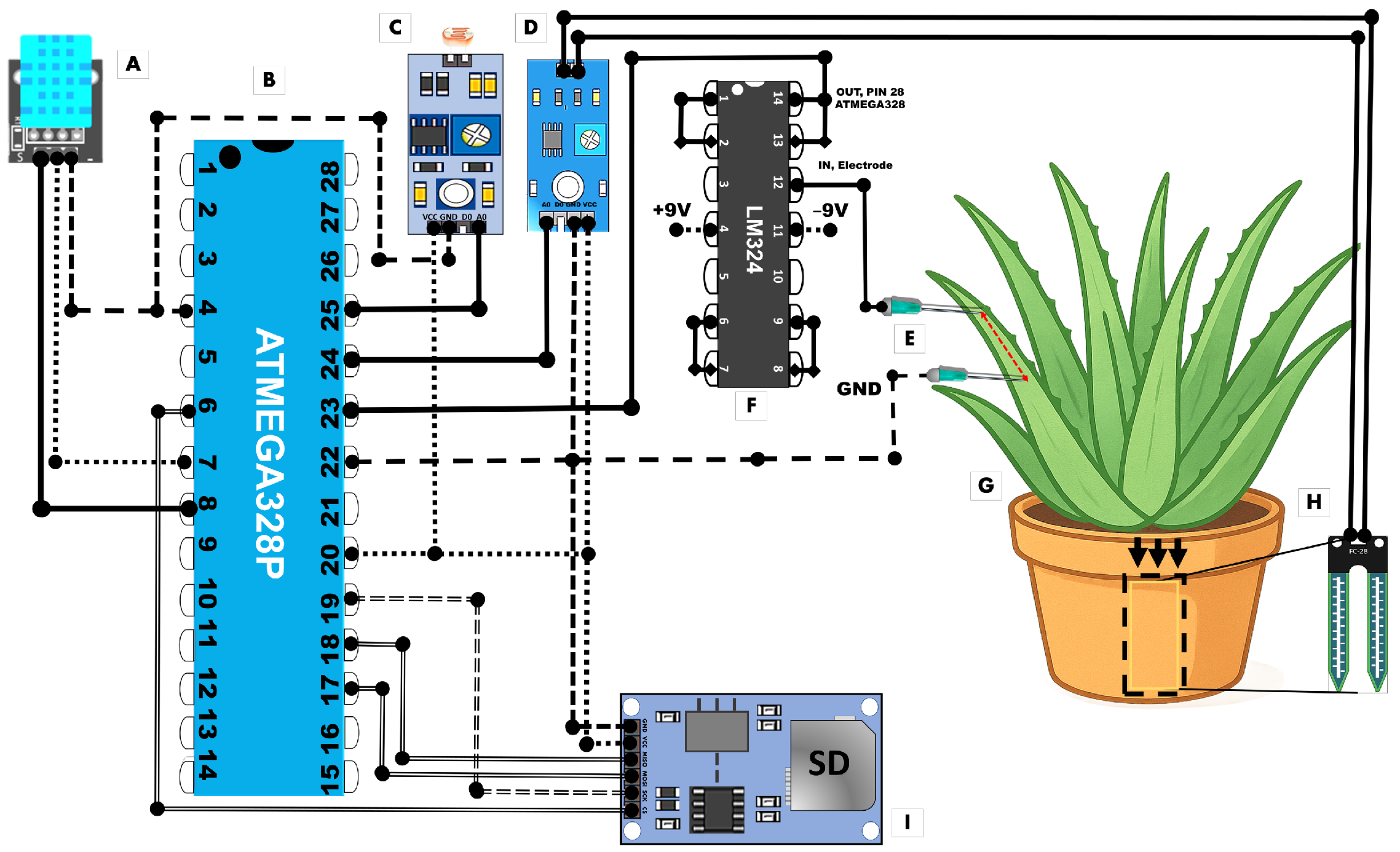
Electronics: A custom-built, low-cost data acquisition system based on the Arduino (Arduino LLC, Somerville, MA, USA) platform was implemented as a cost-effective alternative to expensive laboratory equipment, providing an accessible solution for educational and research environments [24]. The system included a DHT11 sensor for ambient temperature and humidity, an LDR module for ambient light measurement (generic, Shenzhen, China), an FC-28 soil moisture sensor embedded in the potting substrate, and a MicroSD memory module (Shenzhen, China) for local data storage. Signal conditioning was carried out using an LM324 operational amplifier (Texas Instruments, Dallas, TX, USA). The total equipment cost was under USD 20, offering a replicable and affordable solution for biosignal acquisition in plant systems (Figure 4) [21,22].

All experiments were performed on healthy, commercially available Aloe vera plants, which are not considered endangered or protected species. No specific institutional or governmental approval was required. The handling of plants followed local and institutional ethical guidelines, ensuring minimal harm and preserving plant viability during and after measurements.

2.2. Signal Acquisition

To acquire the electrical signals from the Aloe vera plant, two stainless steel electrodes were inserted into a single leaf at specific locations, one near the base and the other near the apex, maintaining a separation distance of 5 cm. The insertion was performed carefully to minimize tissue damage and ensure reliable signal capture. The signals were recorded using the Arduino-based acquisition system previously described, configured with a sampling frequency of 10 Hz. Data were stored on a microSD card for subsequent analysis. Prior to each acquisition session, a stabilization period of 45 min was allotted to allow the plant’s physiological response to adapt following electrode insertion. This waiting time was essential to minimize the influence of transient artifacts and to ensure the recording of representative bioelectrical activity.

2.3. Signal Preprocessing

Prior to analysis, the raw electrical signals acquired from the Aloe vera plant required a preprocessing stage to ensure data quality and consistency. This step is essential for removing noise, outliers, and artifacts that commonly affect bioelectrical measurements [10,11].

The preprocessing of the electrical signal from the Aloe vera plant was carried out in a standardized pipeline to ensure its correct characterization. The raw signals were first inspected visually to identify and note segments with visible motion artifacts or abrupt changes in the baseline. These segments were excluded from further analysis if the deviation exceeded ±3 standard deviations from the baseline amplitude.

Signals were then band-pass-filtered using a 4th-order zero-phase Butterworth filter with a passband of 0.1–10 Hz to remove DC offsets and high-frequency noise unrelated to physiological processes [25,26]. The filter was implemented using the scipy.signal.filtfilt function (SciPy developers, Austin, TX, USA) to avoid phase distortion.

Following filtering, signals were normalized to zero mean and unit variance to standardize the amplitude across plants and sessions. From each coefficient set, statistical features including mean, standard deviation, variance, energy, and Shannon entropy were computed.

The complete preprocessing workflow, including artifact detection thresholds, filter parameters, and feature extraction steps, is provided in the Supplementary Materials (Algorithm S1). This preprocessing pipeline ensured that the signals analyzed in later stages accurately reflected the underlying physiological states of the plant, laying the foundation for reliable feature extraction and classification.

2.3.1. Determination of the Randomness of the Electrical Signal

A signal is considered random if it cannot be precisely predicted, and its values are determined by probabilistic processes. To evaluate the randomness of the electrical signal recorded from the Aloe vera plant, the autocorrelation function was used. This metric quantifies the similarity between a signal and a time-shifted version of itself. For a truly random signal, autocorrelation should approach zero for all non-zero lags, since no repeating pattern should exist [8,14].

The autocorrelation function of the plant’s electrical signal is denoted as $x\left(t\right)$ and, for a time lag $\tau$, is defined in Equation (1):

$$R_x\left(\tau \right)=\mathbb{E}[x\left(t\right)·x(t+\tau )]$$

(1)

where

• $R_x\left(\tau \right)$ is the autocorrelation function at lag $\tau$.
• $\mathbb{E}$ denotes the expected value, which in the discrete case corresponds to the average product of the signal and its shifted version.
• $x\left(t\right)$ is the value of the signal at time t.

For the discrete case, the autocorrelation for N signal samples is given by

$$R_x\left(\tau \right)={\displaystyle \frac{1}{N-\tau }}\sum _{n=0}^{N-\tau -1}x\left[n\right]·x[n+\tau ]$$

(2)

where

• N is the total number of samples.
• $\tau$ is the lag value.
• $x\left[n\right]$ is the value of the signal at time n.

The resulting autocorrelation was visualized using a stem plot, which clearly showed the absence of significant correlation at non-zero lags—confirming the random-like behavior of the signal, as similarly observed in plant electrophysiological studies [10,11].

2.3.2. Determination of the Non-Stationarity of the Electrical Signal

To confirm whether the Aloe vera plant’s electrical signal exhibits non-stationarity, its statistical properties—such as mean and variance—were assessed over time. Non-stationary signals are characterized by temporal changes in these statistical properties, which is a typical feature of bioelectrical activity in living systems [14].

The Augmented Dickey–Fuller (ADF) test was employed to determine the presence of a unit root in the signal, which indicates non-stationarity. The ADF model applied to the data is defined in Equation (3):

$$\Delta y_t=\alpha +\beta t+\sigma y_{t-1}+\sum _{i=1}^p{\delta }_i\Delta y_{t-i}+{\epsilon }_t$$

(3)

where

• $\Delta y_t$ is the first difference of the time series.
• $\alpha$ is a constant term.
• $\beta t$ represents the time trend component.
• $\sigma y_{t-1}$ indicates the autoregressive component.
• ${\delta }_i$ are the coefficients of the lagged differences.
• ${\epsilon }_t$ is the white noise term.

If the null hypothesis is not rejected ($\sigma =0$), the signal is considered non-stationary. The test results confirmed that the electrical signal possessed time-dependent statistical behavior, consistent with previous works on plant electrophysiology [11,22].

2.3.3. Determination of the Nonlinearity of the Electrical Signal

To assess the nonlinear characteristics of the electrical signal, the Broock–Dechert– Scheinkman (BDS) test was performed. This test examines whether the structure of a time series deviates from the assumption of independence and identically distributed (i.i.d.) data, thus revealing hidden nonlinear patterns that cannot be captured by linear methods such as autocorrelation [27].

The BDS statistic is defined by Equation (4):

$$BD{S}_m\left(c\right)={\displaystyle \frac{\sqrt{T}}{{\widehat{\sigma }}_m}}\left[c_m\left(c\right)-C_1{\left(ϵ\right)}^m\right]$$

(4)

where

• $c_m\left(c\right)$ is the correlation integral in dimension m.
• $C_1{\left(ϵ\right)}^m$ is the expected frequency of close points under the i.i.d. hypothesis.
• ${\widehat{\sigma }}_m$ is the estimated standard deviation of the correlation integral.

A significantly low p-value from the test suggested strong evidence of nonlinearity in the signal structure, further supporting the use of non-parametric methods for feature extraction.

2.3.4. Long-Term Correlation Analysis Using Detrended Fluctuation Analysis (DFA)

To evaluate the existence of long-range correlations in the electrical signal, Detrended Fluctuation Analysis (DFA) was conducted. This method is widely used for signals with complex temporal structures and non-stationary behavior, including physiological and environmental time series [22,28].

The implementation used the Python nolds library (version 3.12.4). Each signal was segmented, and local linear trends were subtracted. Then, the root-mean-square fluctuation $F\left(s\right)$ was computed for each window size s, and the log–log relationship between $F\left(s\right)$ and s was used to estimate the scaling exponent $\alpha$.

• $\alpha \approx 0.5$: Uncorrelated behavior (white noise).
• $\alpha >0.5$: Persistent long-term correlations.
• $\alpha <0.5$: Anti-persistent behavior.

The DFA exponent served as a scalar feature to describe temporal memory and was later incorporated into the classification model to detect structural changes due to lead contamination in Aloe vera plants [13,21].

2.4. Non-Parametric Analysis

To characterize the electrical signal of the Aloe vera plant in response to lead contamination, three non-parametric techniques were employed: time-domain statistical analysis, frequency analysis using the Short-Time Fourier Transform (STFT), and time–frequency analysis via the discrete wavelet transform (DWT) and Empirical Mode Decomposition (EMD). These methods are well-suited for analyzing nonlinear and non-stationary biosignals such as those generated by plants under stress conditions [10,21,22].

2.4.1. Time-Domain Analysis

Time-domain features provide a basic but essential overview of the signal. Several statistical metrics were computed, including mean value, maximum, minimum, peak-to-peak amplitude, variance, and the number of zero crossings. The zero-crossing count was defined as the number of times the signal crossed its mean value, capturing the frequency of oscillatory activity within the plant.

These metrics have been shown to be useful in distinguishing normal physiological activity from stress-induced changes in plant signals [11,27]. Moreover, prior studies demonstrate that shifts in these values are often associated with the presence of environmental contaminants [8,13].

Preliminary STFT tests confirmed a dominance of low-frequency components in the signal, consistent with previous observations in plant electrophysiology [14]. However, due to STFT’s fixed window size and limited time–frequency resolution, advanced adaptive methods like DWT and EMD were prioritized for feature extraction [22].

2.4.2. Time–Frequency-Domain Analysis

The discrete wavelet transform (DWT) was used to capture the temporal and spectral characteristics of the signal across multiple scales. The transformation is defined as follows:

$$W_{\psi }(a,b)=\sum _{n=-\infty }^{\infty }x\left[n\right]{\psi }_{a,b}\left[n\right]$$

(5)

where $W_{\psi }(a,b)$ denotes the wavelet coefficient, $x\left[n\right]$ is the discrete signal, and ${\psi }_{a,b}\left[n\right]$ is the scaled and shifted wavelet function. Here, a and b represent the scale and translation parameters, respectively.

The “db3” mother wavelet from the Daubechies family was selected due to its compact support and effectiveness in capturing signal singularities in biosignals [22]. The signal was decomposed into 5 levels, each revealing different frequency components and transients.

The decomposition was performed using Python 3.12.4 and the PyWavelets library (version 1.5.0; PyWavelets Developers, USA), producing a spectrum that provided insights into the dynamic behavior of the Aloe vera electrical signal across frequency bands. This approach has been effectively used in prior biosignal studies for detecting subtle and localized variations in physiological signals [19].

2.4.3. Signal Decomposition Using Empirical Mode Decomposition (EMD)

To further characterize the nonlinear and non-stationary structure of the signal, Empirical Mode Decomposition (EMD) was applied. EMD is particularly effective for biosignal analysis because it does not require a predefined basis, instead extracting components (IMFs) that are intrinsic to the data itself [22,29].

Each signal was decomposed into a finite number of intrinsic mode functions (IMFs) and a residual trend:

$$x\left(t\right)=\sum _{i=1}^n{\mathrm{IMF}}_i\left(t\right)+r\left(t\right)$$

(6)

where

• $x\left(t\right)$ is the original signal;
• ${\mathrm{IMF}}_i\left(t\right)$ is the i-th intrinsic mode function;
• n is the number of IMFs;
• $r\left(t\right)$ is the residual trend.

The process was implemented in Python using the PyEMD library (v1.2.1). Local extrema were identified and interpolated with cubic splines to generate upper and lower envelopes, followed by iterative sifting. The stopping criterion was a standard deviation threshold of 0.2, producing six IMFs and one residue per signal.

From each IMF, the following features were extracted:

• Energy: $E_i={\sum }_k{\mathrm{IMF}}_i{\left(k\right)}^2$, quantifying the power contribution of each IMF.
• Shannon Entropy: Computed from the amplitude distribution of each IMF to evaluate its internal complexity.

These features were normalized and used as inputs to the machine learning models. The use of EMD in plant electrophysiology has gained traction for its capacity to isolate relevant patterns under stress conditions, including contamination [22,29].

2.5. Parametric Analysis

After uncovering key signal dynamics via non-parametric methods, the electrical signal of the Aloe vera plant was modeled parametrically using autoregressive (AR) models. AR models are well-suited for time-series analysis, expressing the current value of a signal as a linear combination of its previous values plus a stochastic error term [10,30].

The AR(p) model is defined as follows:

$$X_t={\varphi }_1{X}_{t-1}+{\varphi }_2{X}_{t-2}+\cdots +{\varphi }_p{X}_{t-p}+{\epsilon }_t$$

(7)

where $X_t$ is the signal value at time t, ${\varphi }_i$ are the lag coefficients, and ${\epsilon }_t$ is white noise. To determine the optimal order p, several models were tested and their performance was evaluated using metrics like the mean squared error (MSE), mean absolute error (MAE), and Akaike Information Criterion (AIC), as recommended in prior studies [9,31]. It was observed that increasing the order improved fit up to a point, after which the benefits diminished—aligning with the findings in plant signal modeling.

The AR approach enables compact temporal characterization and prediction of signal behavior, complementing wavelet-based methods that excel in capturing transients [31].

2.6. Feature Extraction

By integrating features from both parametric and non-parametric analyses, a comprehensive feature set was generated to characterize changes in the plant’s electrical response to lead exposure.

2.6.1. Non-Parametric Features (from DWT)

• Energy per scale: Power distribution across wavelet levels, indicating changes in physiological activity [22].
• Wavelet coefficients: Time-localized amplitude features sensitive to transient events.
• Entropy per level: Shannon entropy to quantify signal irregularity across scales [22].
• Dominant frequency: Main spectral components at each condition, reflecting low-frequency dominance in plant electrical responses [14].

2.6.2. Parametric Features (from AR(10))

• AR coefficients (${\varphi }_1$–${\varphi }_{10}$): Capturing the signal’s autoregressive dynamics [7,31].
• Residual variance: Quantifying the unpredictability and fit error of the model [9].
• Time-domain statistics: Mean, median, standard deviation, and zero crossings to capture overall signal fluctuations.

2.6.3. Nonlinear Complexity Features

• Shannon entropy: Derived from both the original signal and EMD-based IMFs to assess disorder [9].
• Permutation entropy: A temporal complexity measure using embedding dimension 5 and delay 1, robust for short and noisy biosignals [32,33].
• Spectral entropy: Computed from the normalized PSD via Welch’s method, capturing spectral distribution irregularity [34].

This multidimensional feature space was specifically designed to detect structural, spectral, and temporal alterations induced by lead contamination. By integrating descriptors from time, frequency, and complexity domains, it characterized plant bioelectrical responses for subsequent classification analysis.

2.7. Classification Algorithm Training

After extracting a comprehensive set of features from the electrical signals of Aloe vera var. Chinensis, a supervised classification strategy was implemented to distinguish between signals from lead-contaminated and uncontaminated plants.

Three classification algorithms were employed in this study: Support Vector Machine (SVM), Random Forest (RF), and Extreme Gradient Boosting (XGBoost). These models were selected for their complementary strengths in analyzing small- to moderate-sized datasets with potentially nonlinear decision boundaries. Specifically, SVM is well established for its robustness in high-dimensional spaces and small-sample settings [35]; RF leverages an ensemble-based strategy that reduces overfitting risk while capturing complex feature interactions [36]; and XGBoost provides state-of-the-art gradient boosting with built-in regularization and efficient treatment of sparse or noisy features [37].

• Support Vector Machine (SVM): A kernel-based algorithm with proven performance on small datasets and high-dimensional spaces. SVM has been employed in several plant biosignal classification studies due to its generalization capacity and robustness under abiotic stress conditions [13,38].
• Random Forest (RF): An ensemble tree-based method widely adopted in environmental and agricultural sciences. RF handles complex feature interactions and offers intrinsic feature importance estimation, which is particularly useful when dealing with multidomain descriptors [36].
• Extreme Gradient Boosting (XGBoost): A scalable and regularized gradient boosting algorithm that outperforms many traditional classifiers in structured data problems. Its capacity for feature attribution through SHAP (SHapley Additive exPlanations) makes it highly valuable in biomedical and environmental applications [22,23]. XGBoost was included among the classifiers because of its demonstrated effectiveness in agricultural and environmental applications, where it has shown strong performance in capturing complex, nonlinear patterns [39].

Hyperparameter tuning was performed for each model using a grid search with stratified 5-fold cross-validation to maximize accuracy while preventing overfitting. The search ranges and selected optimal values are summarized in

Table 1. Optimal hyperparameters for each classification model obtained via grid search with stratified 5-fold cross-validation.

Model	Hyperparameter	Optimal Value
SVM	Kernel	RBF
	C (regularization)	10
	Gamma	0.01
Random Forest	Number of trees (n_estimators)	200
	Max depth	8
	Min samples split	4
	Max features	sqrt
XGBoost	Number of trees (n_estimators)	300
	Max depth	6
	Learning rate	0.05
	Subsample	0.8
	Colsample by tree	0.8
	Gamma	0.1

. This tuning process ensured that reported performance metrics reflect well-optimized models rather than default configurations.

The dataset consisted of 320 labeled instances: 160 from Pb-contaminated plants (class 1) and 160 from the control (class 0). Each instance included a feature vector comprising wavelet-derived attributes, AR model coefficients, entropy measures, and basic time-domain statistics. A final hold-out test set of 64 instances (32 per class) was reserved for independent evaluation, while the remaining 256 instances (128 per class) were used for model training and hyperparameter tuning via stratified 5-fold cross-validation.

Stratified sampling was used to preserve class distribution. Data processing and model training were implemented in Python 3.12.4 using the libraries scikit-learn, pandas, numpy, and xgboost.

For the best-performing model (XGBoost), SHAP values were computed to provide insight into the contribution of each feature to classification outcomes. This interpretability supports explainable AI (XAI) practices, ensuring that the predictions are grounded in physiologically meaningful variables [23].

2.8. Validation and Evaluation of the Classification Algorithm

The classification performance was evaluated using a stratified 5-fold cross-validation strategy. cross-validation strategy applied exclusively to the training set (256 instances: 128 per class). In each fold, the model was trained on 80% of the training data and validated on the remaining 20%. Hyperparameter tuning was carried out using grid search optimization via GridSearchCV, targeting maximum accuracy. After hyperparameter optimization, the final model was retrained on the complete training set and evaluated on the independent hold-out test set of 64 instances (32 per class).

The following standard classification metrics were computed:

• Accuracy: Overall proportion of correctly predicted instances.

  $$\mathrm{Accuracy}={\displaystyle \frac{TP+TN}{TP+TN+FP+FN}}$$

  (8)
• Precision: Proportion of predicted positives that were actually positive.

  $$\mathrm{Precision}={\displaystyle \frac{TP}{TP+FP}}$$

  (9)
• Recall (Sensitivity): Fraction of actual positives correctly identified.

  $$\mathrm{Recall}={\displaystyle \frac{TP}{TP+FN}}$$

  (10)
• F1-Score: Harmonic mean of precision and recall.

  $$F1={\displaystyle \frac{2·\mathrm{Precision}·\mathrm{Recall}}{\mathrm{Precision}+\mathrm{Recall}}}$$

  (11)

Additionally, a confusion matrix was constructed to visualize classification outcomes.

Model interpretability was further enhanced using SHAP value analysis for XGBoost. SHAP plots allowed visualization of the individual and cumulative effect of each feature (e.g., wavelet entropy, AR variance, and IMF-based complexity) on the classifier’s decision. These tools help clarify how plant electrical signals reflect physiological responses to environmental toxins such as lead [22,23].

The Python scripts developed for this study cannot be made publicly available due to intellectual property restrictions. However, all algorithms, parameter settings, and processing steps are described in sufficient detail within the manuscript to enable independent reproduction of the analyses.

3. Results and Discussion

3.1. Electrical Control Signal and Electrical Signal Contaminated with Lead

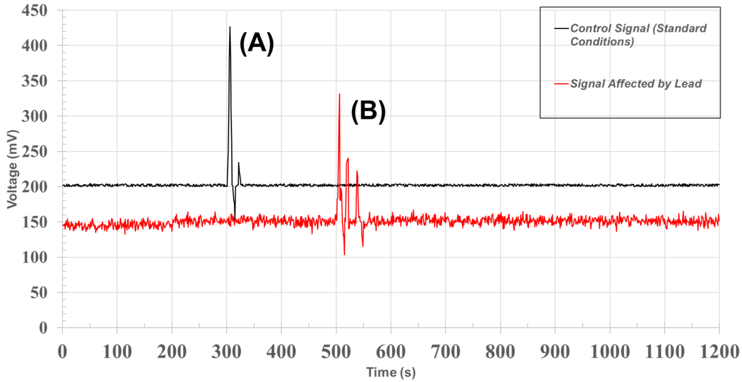
A total of 320 electrical signals were recorded from 160 plants of Aloe vera var. Chinensis. The control signals, which were consistent with previous reports [31,40], showed clear differences from the signals of lead-exposed plants. These differences in dynamic behavior were statistically significant across all specimens, as illustrated in Figure 5.

The results demonstrate consistent and reproducible differences in signal morphology between control and lead-exposed plants. This behavior can be explained by the disruptive effect of heavy metals like lead on physiological processes, particularly those involving ion transport, cellular excitability, and membrane potential regulation [8,14]. Lead ions are known to interfere with calcium signaling and potassium channel activities, which are critical in the generation and propagation of bioelectrical signals in plant tissues [22,41].

Consistent with these physiological disruptions, the contaminated signals exhibited a noticeable reduction in amplitude and temporal variability across all recordings. Such a reduction aligns with findings in other biosignal studies where metal-induced oxidative stress and membrane depolarization dampen the bioelectrical activity of plant systems [13,27]. Importantly, the graphical contrast between the two signal classes indicates that lead contamination produces a systematic and measurable alteration in the signals, rather than random noise or recording artifacts [42].

This consistent visual difference in signal morphology supports the view that bioelectrical signals can act as reliable indicators of environmental stress, particularly under trace metal contamination [21]. As shown in Figure 6, box plots and density plots provide a visual comparison of the two signal classes, illustrating the differences observed in their distributions.

The control group exhibited an average amplitude of 201.95 mV (SD ± 9.84), indicating consistent signal levels with low variability across plants. In contrast, the lead-contaminated signal averaged 150.52 mV (SD ± 8.91), indicating a substantial decrease of approximately 25.4%. These results are consistent with previously reported trends in bioelectrical signal suppression due to metal stress [10,11].

From a mechanistic standpoint, this attenuation may arise from lead-induced inhibition of H⁺-ATPase activity and impaired ionic balance across membranes, which in turn reduces the membrane potential fluctuations necessary to generate measurable signals [14]. This result, observed consistently across the sample of plants, supports the potential of Aloe vera as a real-time biosensor for detecting lead in different environments.

Furthermore, the reproducibility of these measurements, obtained with a low-cost Arduino-based monitoring system, demonstrates the practicality of biosensing with plant electrical signals for environmental diagnostics [21,22].

3.2. Signal Preprocessing

To assess the quality and characteristics of the electrical signal captured from Aloe vera, several statistical and dynamical tests were applied to validate its suitability for further analysis and classification. Specifically, the randomness, non-stationarity, nonlinearity, and long-range correlations were examined, as these are typical properties of bioelectrical signals in plant physiology [22].

The first test assessed the randomness of the signal using autocorrelation analysis. The autocorrelation function $R_x\left(\tau \right)$ was computed for different lags $\tau$ using Equation (2). In the implementation, a Python-based routine calculated the products $x\left[n\right]·x[n+\tau ]$ and normalized the sum over the total effective length $N-\tau$.

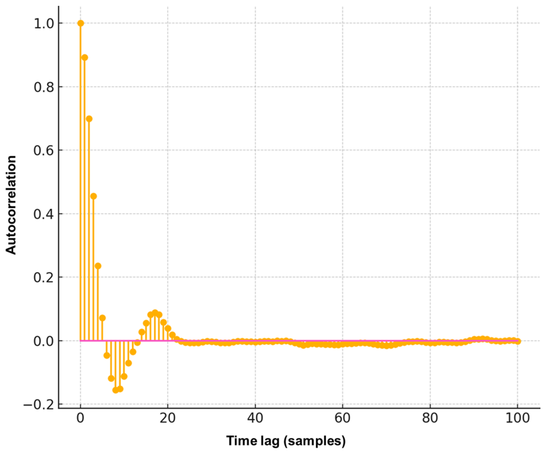
To visualize this analysis, a stem plot was used (Figure 7), which is suitable for discrete data and highlights how signal correlations decay across time lags.

Figure 7 shows that for $\tau =0$, $R_x\left(0\right)$ reaches its maximum, while subsequent lags quickly decay toward zero. This confirms that the electrical signal does not follow a repetitive pattern, which is indicative of a random process—a known characteristic in biological and plant electrophysiological signals [10,14].

Next, the Augmented Dickey–Fuller (ADF) test (Equation (3)) was applied to assess whether the signal was stationary or exhibited time-dependent trends. The results yielded a test statistic of $\tau =-1.85$ and a p-value of $p=0.36$. Since $p>\alpha =0.05$ and $\tau$ was greater than the critical values at the 1%, 5%, and 10% levels, the unit-root null hypothesis could not be rejected. This indicates that the signal is non-stationary, consistent with the time-varying characteristics commonly observed in physiological processes of plants under external stress [8,21].

The analysis yielded a BDS statistic of $BDS=28.1$, with a z-score of $z=50.12$ and a standard deviation of $\sigma =0.46$. Since $z\gg z_{\alpha =0.05}=1.96$, the null hypothesis of linear independence was rejected, indicating nonlinear dynamics in the signal.

This aligns with other studies showing that plant electrophysiological signals typically display nonlinear dynamics due to the complex interplay of ion transport, membrane polarization, and environmental feedback mechanisms [11,27].

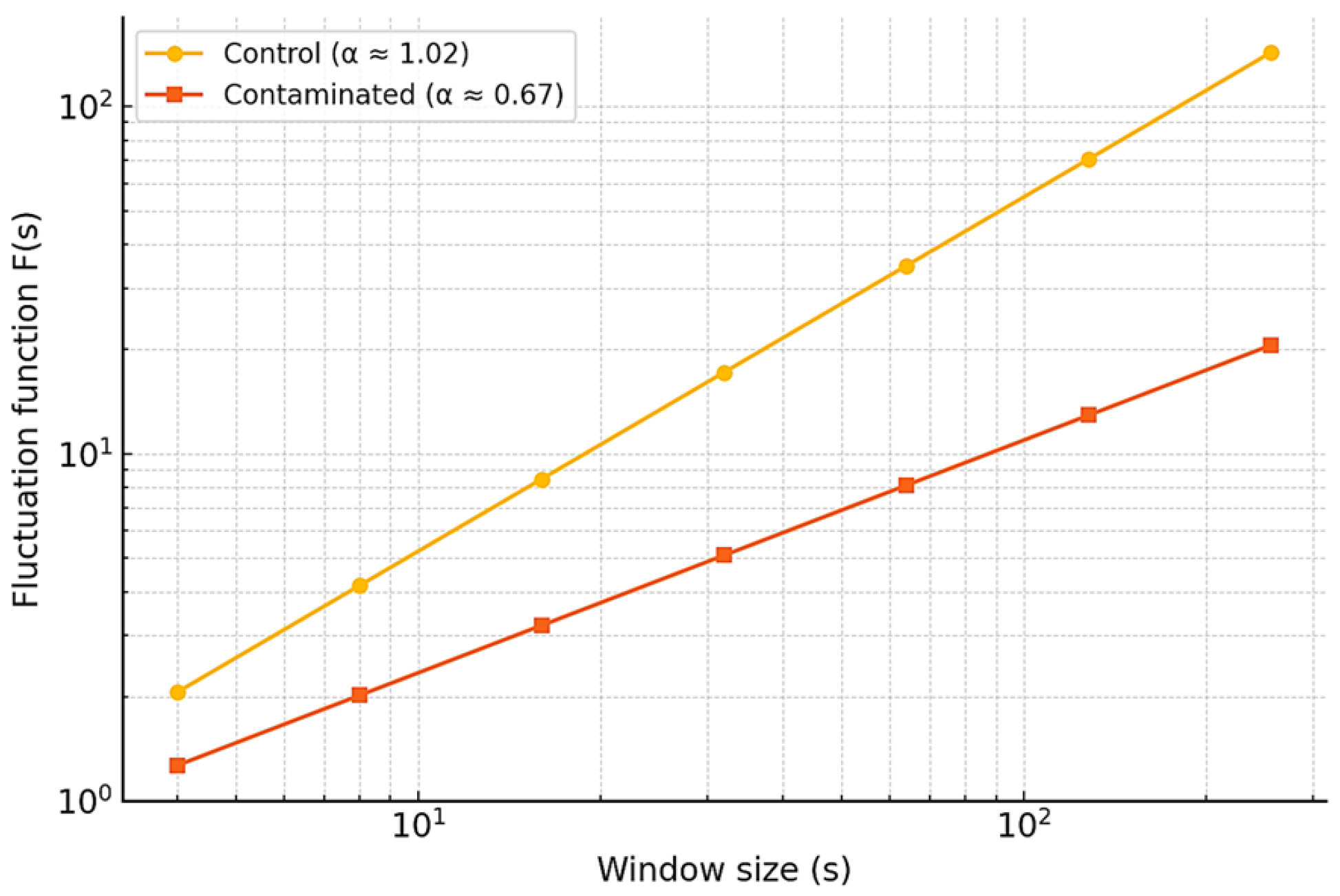
To evaluate long-range temporal correlations, Detrended Fluctuation Analysis (DFA) was applied. This method quantifies how signal fluctuations scale with window size, providing an estimate of persistence across time.

For control signals, the DFA exponent was $\alpha =1.02\pm 0.04$, consistent with persistent correlations and stable temporal organization. In contrast, Pb-contaminated signals showed a lower exponent of $\alpha =0.67\pm 0.07$, reflecting disrupted structure and anti-persistent dynamics (Figure 8). Similar alterations have been reported in plants under metal stress, where reduced $\alpha$ values are associated with impaired physiological regulation [13,41].

Overall, the signal preprocessing results confirmed that the acquired electrical signals exhibit the expected characteristics described in the literature for biosignals in plants—namely randomness, non-stationarity, nonlinearity, and distinct scaling behaviors—supporting their suitability for advanced time-series analysis and classification.

3.3. Non-Parametric Analysis

A comparative analysis of the electrical signals in the time domain was conducted on the 320 measured signals (160 control and 160 contaminated) to evaluate the effects of lead contamination on the Aloe vera plant.

Table 2. Time-domain statistical metrics comparing control and lead-contaminated Aloe vera signals.

Metric	Control (No Pb)	Contaminated (Pb)
Mean Value	202.85 mV	151.10 mV
Maximum	428.12 mV	332.45 mV
Minimum	149.87 mV	102.98 mV
Peak-to-Peak	278.25 mV	229.47 mV
Variance	126.85 mV2	125.93 mV2
Zero Crossings	507 times	472 times

summarizes key statistical metrics for both conditions.

The control signal exhibited higher baseline values and greater peak amplitudes, suggesting more robust electrical activity. In contrast, the contaminated signal showed reduced mean and peak values, indicating a suppression of physiological processes potentially related to ionic imbalance caused by heavy metals [41]. Despite similar variance values, a smaller peak-to-peak range in the contaminated signals suggests a compression of their dynamic range. This is consistent with previous studies reporting the damping effect of metal toxicity on plant bioelectric responses [13].

3.4. Wavelet-Based Time–Frequency Analysis

The discrete wavelet transform (DWT) was applied to the electrical signal of the Aloe vera plant using the Daubechies 3 (db3) mother wavelet and five decomposition levels. This method is particularly effective for non-stationary signals, as it captures both temporal and frequency-domain features simultaneously, which is essential for characterizing plant physiological responses under stress [22,43,44].

Figure 9 shows a 3D representation of the multi-level wavelet decomposition. The horizontal axis corresponds to time (s), the depth axis to decomposition level (dimensionless), and the vertical axis to coefficient magnitude (a.u.). The black trace at the base represents the original contaminated signal, which shows a clear perturbation around 450 s corresponding to Pb application.

In the decomposed representation, lower levels (L1–L2) exhibit low-amplitude, high-frequency components, consistent with baseline electrophysiological activity. In contrast, higher levels (L4–L5) show pronounced peaks between 200 and 500 s, associated with transient ionic fluxes and localized stress responses under Pb exposure [11,27]. These high-energy events are consistent with rapid depolarization–repolarization cycles in excitable plant tissues, likely influenced by calcium and potassium channel activity.

The multiscale resolution of the DWT allows the identification of short-lived electrical responses that are often missed by single-scale approaches. This highlights the value of DWT-derived metrics—such as energy distribution, entropy, and dominant frequency bands—as indicators for distinguishing control from Pb-contaminated signals [22,45].

3.5. Signal Decomposition Using Empirical Mode Decomposition (EMD)

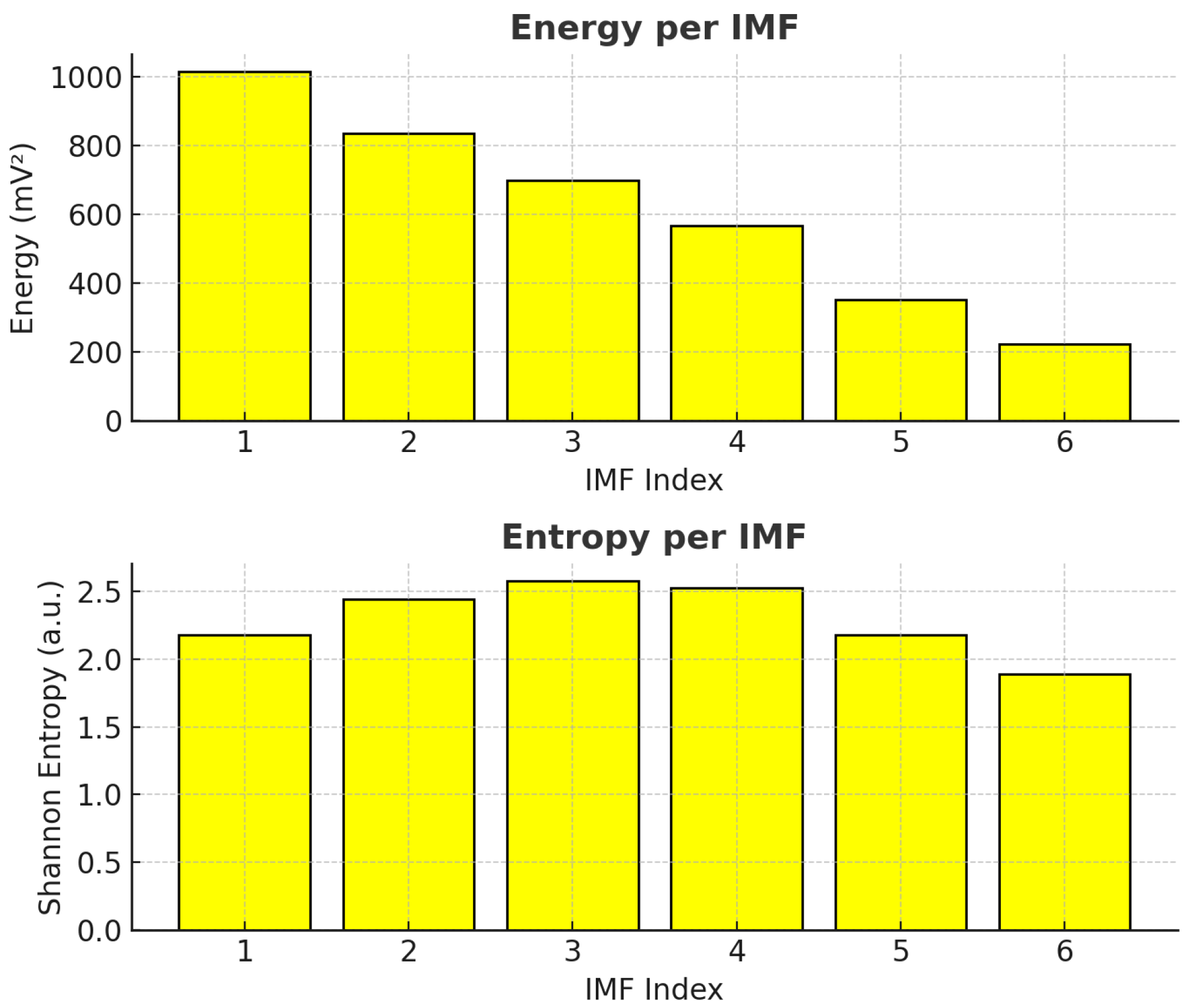
Empirical Mode Decomposition (EMD) was applied to isolate intrinsic signal components. Six intrinsic mode functions (IMFs) were consistently extracted from the electrical signal, along with a residual component. The energy and Shannon entropy of each IMF were computed (

Table 3. Energy and Shannon entropy for each IMF obtained from the EMD of a representative Aloe vera signal.

IMF Index	Energy	Shannon Entropy
1	1012.47	2.182
2	838.62	2.441
3	702.15	2.573
4	568.08	2.529
5	355.34	2.174
6	224.11	1.889

and Figure 10) to evaluate their contribution and complexity. This technique has been successfully used in physiological signal studies to characterize nonlinear responses under environmental stress [22].

The trend in energy confirms that IMF1 accounts for the most dynamic, high-frequency signal components. In contrast, entropy peaked in intermediate IMFs (IMF 2 to 4), suggesting these modes reflect rich, irregular activity—likely corresponding to adaptive electrophysiological responses of the plant under contamination. These observations align with prior applications of EMD in non-invasive biosensing and open opportunities for refined classification based on mode-specific dynamics [46].

3.6. Parametric Analysis

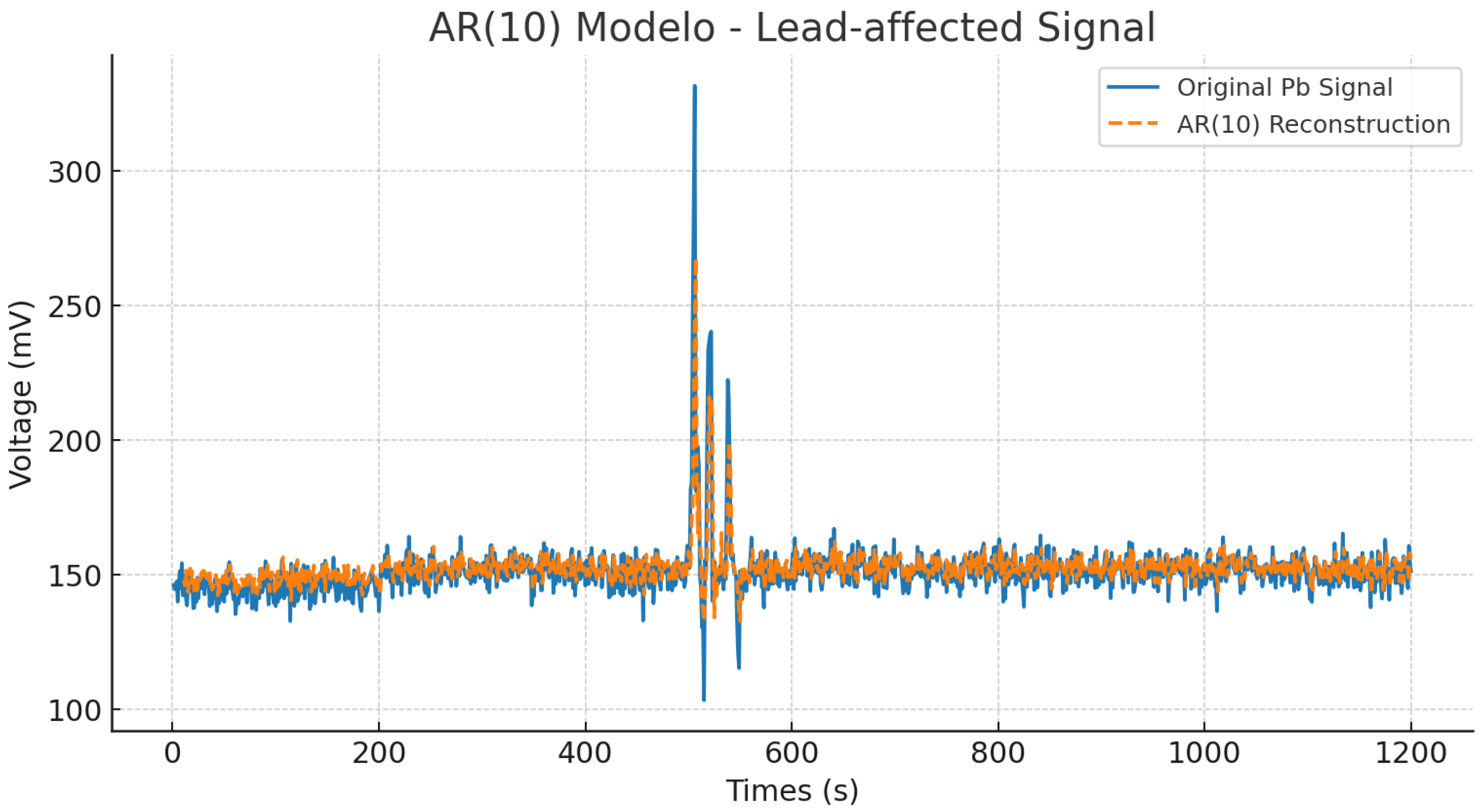
To model the temporal dynamics of the lead-contaminated Aloe vera electrical signal, an autoregressive model of order 10 (AR(10)) was implemented. This model estimates the current value of the signal $x\left(n\right)$ based on a weighted combination of its 10 previous samples, as expressed in Equation (12).

$$\begin{array}{cc}\hfill x\left(n\right)=& 52.845+0.605x(n-1)+0.092x(n-2)-0.051x(n-3)\hfill \\ \hfill & +0.068x(n-4)-0.095x(n-5)+0.037x(n-6)\hfill \\ \hfill & -0.028x(n-7)+0.023x(n-8)-0.114x(n-9)\hfill \\ \hfill & +0.121x(n-10)+ϵ\left(n\right)\hfill \end{array}$$

(12)

The model was trained on the contaminated signal using least-squares estimation. Figure 11 compares the original signal and the AR(10)-based reconstruction. The AR model captures the general trend and amplitude envelope with high fidelity, including transient fluctuations around index 500 (time), where the signal exhibits strong perturbations likely caused by lead-induced physiological stress.

Quantitatively, the AR(10) model achieved a mean squared error of $MSE=6.2$, a mean absolute error of $MAE=1.5$, and a coefficient of determination of $R^2=0.94$. These values indicate that the model effectively captures the underlying linear structure of the signal, despite the non-stationary and noisy characteristics of biological data. Low error values confirm its predictive ability, while the $R^2$ close to unity reflects correct performance.

These results indicate that the AR(10) model is highly effective in capturing the underlying linear structure of the signal, despite the non-stationary and noisy nature of biological data. The relatively low error metrics confirm its predictive capability, while the $R^2$ value close to 1 suggests excellent fitting.

AR modeling has been widely used in plant electrophysiology to approximate physiological patterns, especially under abiotic stress or toxic exposure, due to its interpretability and capacity to quantify temporal dependencies [46,47,48,49]. Studies have shown that AR models not only reduce computational complexity but also retain physiologically meaningful coefficients that can be linked to the presence of environmental contaminants [50].

This parametric representation provided valuable features that were later used as input for classification algorithms. Furthermore, the AR model serves as a low-complexity, interpretable tool for real-time biosignal synthesis, anomaly detection, and adaptive filtering in intelligent biosensing systems [51].

3.7. Overview of Extracted Features

Table 4. Summary of extracted features, their methodological origin, functional meaning, and relevance to signal characterization.

Feature	Origin	Description	Relevance
Wavelet Energy (per level)	DWT	Signal energy across decomposition scales	Identifies frequency bands where Pb alters dynamics
Wavelet Coefficients	DWT	Localized time–frequency amplitudes	Capture transient physiological events
Entropy (per scale)	DWT	Complexity within each wavelet level	Measures irregularity under stress
Dominant Frequency	DWT/FFT	Highest-energy frequency component	Tracks spectral shift due to Pb interference
AR Coefficients (${\varphi }_i$)	AR Model	Weights on past values in signal prediction	Model temporal dependencies and dynamics
Residual Error Variance	AR Model	Unexplained variability by AR model	Indicates unpredictability under contamination
Mean/Median/Std	Time Domain	Central tendency and dispersion	General statistical description of signal
Zero Crossings	Time Domain	Sign changes around the mean	Indicates oscillatory activity level
Shannon Entropy (IMFs)	EMD	Complexity of intrinsic oscillatory modes	Reflects signal richness and stress response
Permutation Entropy	Nonlinear	Temporal unpredictability	Sensitive to disordered dynamics from Pb
Spectral Entropy	Frequency Domain	Distribution of power across frequencies	Summarizes energy dispersion over spectrum
DFA Exponent ($\alpha$)	DFA	Scaling of long-term fluctuations	Detects loss of temporal organization under stress

summarizes the most relevant features extracted from the electrical signals of the Aloe vera plants under both control and contaminated conditions. Each feature is classified by its origin (methodological domain), described according to its functional role, and contextualized in terms of its importance for classification or physiological interpretation.

The integration of multiple domains (time, frequency, nonlinear, and parametric) enhances signal interpretability and provides a richer representation of the plant’s response to stress. Previous studies have demonstrated that such feature fusion can significantly improve biosignal classification accuracy while preserving physiological interpretability [52,53,54]. In this study, combining wavelet-based energy descriptors with AR model coefficients and entropy metrics proved especially valuable for discriminating lead-induced disruptions.

3.8. Classification Algorithm Performance and Confusion Matrix Analysis

Table 5. Comparative evaluation metrics for the classification algorithms.

Metric	SVM	Random Forest	XGBoost
Accuracy	0.88	0.93	0.96
Precision	0.90	0.91	0.94
Recall	0.82	0.91	0.94
F1-Score	0.86	0.91	0.94

summarizes the evaluation metrics for the three classifiers. XGBoost obtained the best overall results, with both precision and recall at 0.94, showing reliable detection of both Pb-contaminated and control signals. SVM reached a precision of 0.90 but a lower recall of 0.82, indicating missed contaminated cases. Random Forest achieved balanced values (precision and recall at 0.91), slightly below XGBoost in accuracy.

To statistically compare model performances, 95% confidence intervals were computed for all evaluation metrics using 1000 bootstrap resamples. Pairwise comparisons between classifiers were performed using the Wilcoxon signed-rank test on the cross-validation fold scores. Additionally, permutation tests ($n=1000$) were conducted to assess the probability of obtaining the observed accuracies under a null hypothesis of label exchangeability.

The results indicated that XGBoost significantly outperformed both SVM and Random Forest in accuracy (p = 0.011 vs. RF, p = 0.007 vs. SVM), precision (p = 0.018 vs. RF, p = 0.013 vs. SVM), and recall (p = 0.017 vs. RF, p = 0.010 vs. SVM). All permutation test p-values were below 0.01, confirming that the observed differences in performance are highly unlikely to be due to random chance.

Table 6. Statistical comparison of classifiers using Wilcoxon signed-rank test (p-values) and permutation tests.

Comparison	Accuracy p-Value	Precision p-Value	Recall p-Value
XGBoost vs. SVM	0.007	0.013	0.010
XGBoost vs. RF	0.011	0.018	0.017
RF vs. SVM	0.078	0.069	0.062

summarizes the statistical comparisons.

These results confirm that XGBoost was the most accurate and balanced model, making it the best option for classifying bioelectrical signals in environmental contamination studies. This aligns with previous studies reporting that XGBoost performs well on small datasets with high-dimensional features [37,55,56].

To assess classification performance, confusion matrices were generated for each model. As shown in Figure 12, all classifiers performed well, with XGBoost showing the best performance.

Based on the confusion matrices shown in Figure 12, additional metrics were calculated to provide a more comprehensive evaluation of classifier performance. In particular, sensitivity (recall) and specificity were assessed to quantify the ability of each model to correctly identify both lead-contaminated and uncontaminated signals. XGBoost achieved the highest sensitivity (0.94) and specificity (0.95), confirming its balanced capability to minimize both false negatives and false positives. Random Forest followed closely with a sensitivity of 0.92 and specificity of 0.94, maintaining strong overall performance. In contrast, SVM exhibited lower sensitivity (0.83) but higher specificity (0.95), indicating a stronger tendency to correctly classify uncontaminated samples while missing a greater proportion of contaminated signals.

These results further support the discussion that XGBoost achieves the most favorable balance between detecting lead-contaminated signals and correctly identifying uncontaminated signals—an essential requirement in environmental monitoring, where both false negatives and false positives must be minimized. The dataset analyzed in this study comprised 320 labeled instances, obtained from two measurements per plant across 80 plants (160 samples per group: control and lead-contaminated).

Subsequently, to smooth out the overfitting, a stratified five-fold cross-validation scheme was combined with 1000 bootstrap resamples to derive mean performance metrics and their 95% confidence intervals. In addition, permutation tests ($n=1000$) were conducted for each classifier to determine the likelihood of achieving the observed classification accuracies under the null hypothesis of label exchangeability. All statistical analyses confirmed that the classification performance was significantly higher than random chance, indicating that the obtained results are robust and unlikely to be explained by statistical artifacts. The bootstrap-derived mean values and 95% confidence intervals for accuracy, precision, recall, and F1-score of the XGBoost model are summarized in

Table 7. Bootstrap-derived mean performance metrics ($n=1000$ resamples) with 95% confidence intervals for the XGBoost classifier.

Metric	Mean	95% CI
Accuracy	0.956	[0.932, 0.978]
Precision	0.940	[0.915, 0.968]
Recall	0.938	[0.910, 0.965]
F1-Score	0.939	[0.912, 0.966]

.

The implementation of three distinct classification algorithms with complementary strengths, combined with systematic hyperparameter tuning via grid search and cross-validation, reduced the likelihood that the observed performance was influenced by the bias of a single model. This methodological approach provides greater confidence that the extracted bioelectrical signal features are genuinely discriminative of lead exposure, rather than artifacts generated by a specific classification technique.

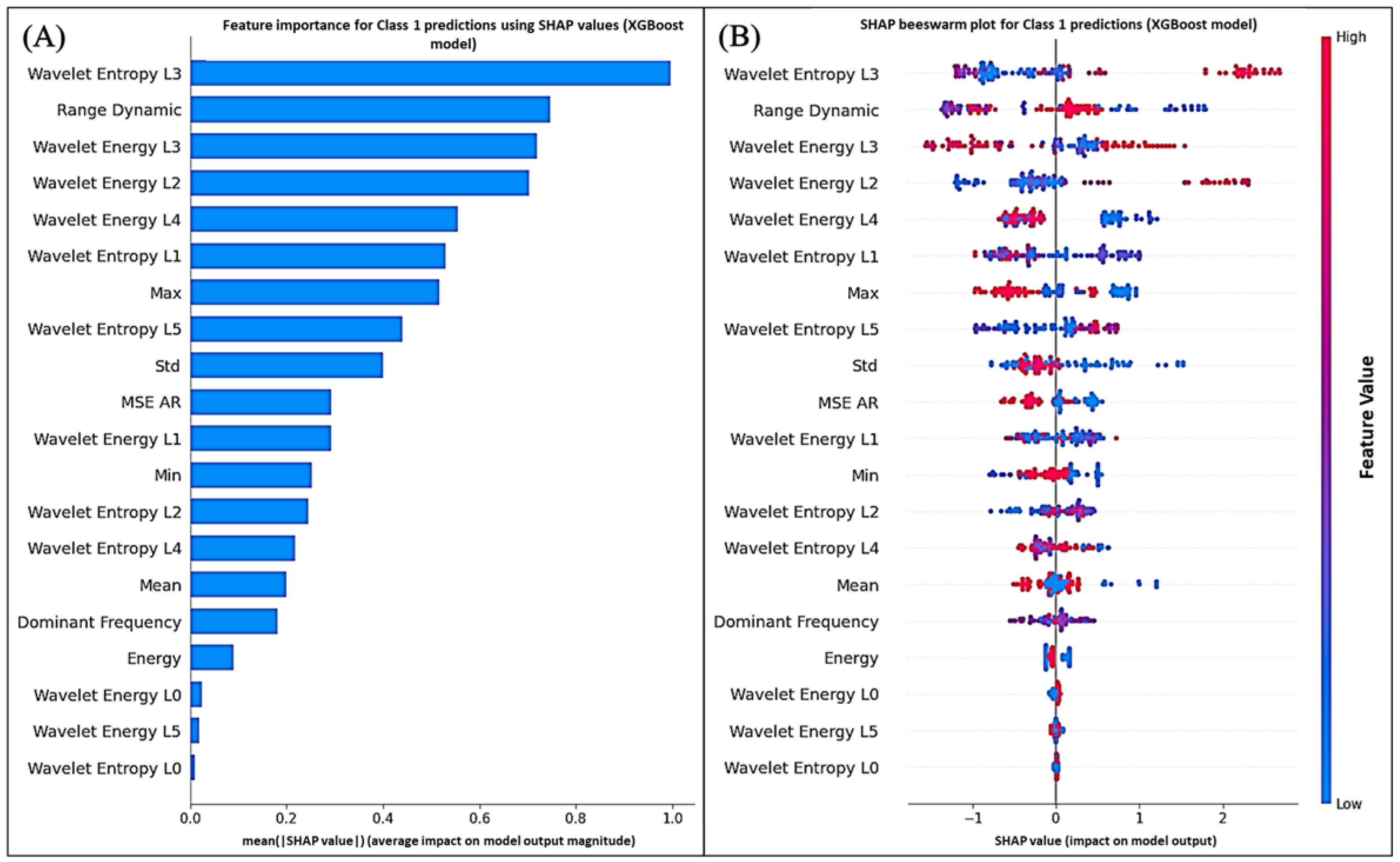
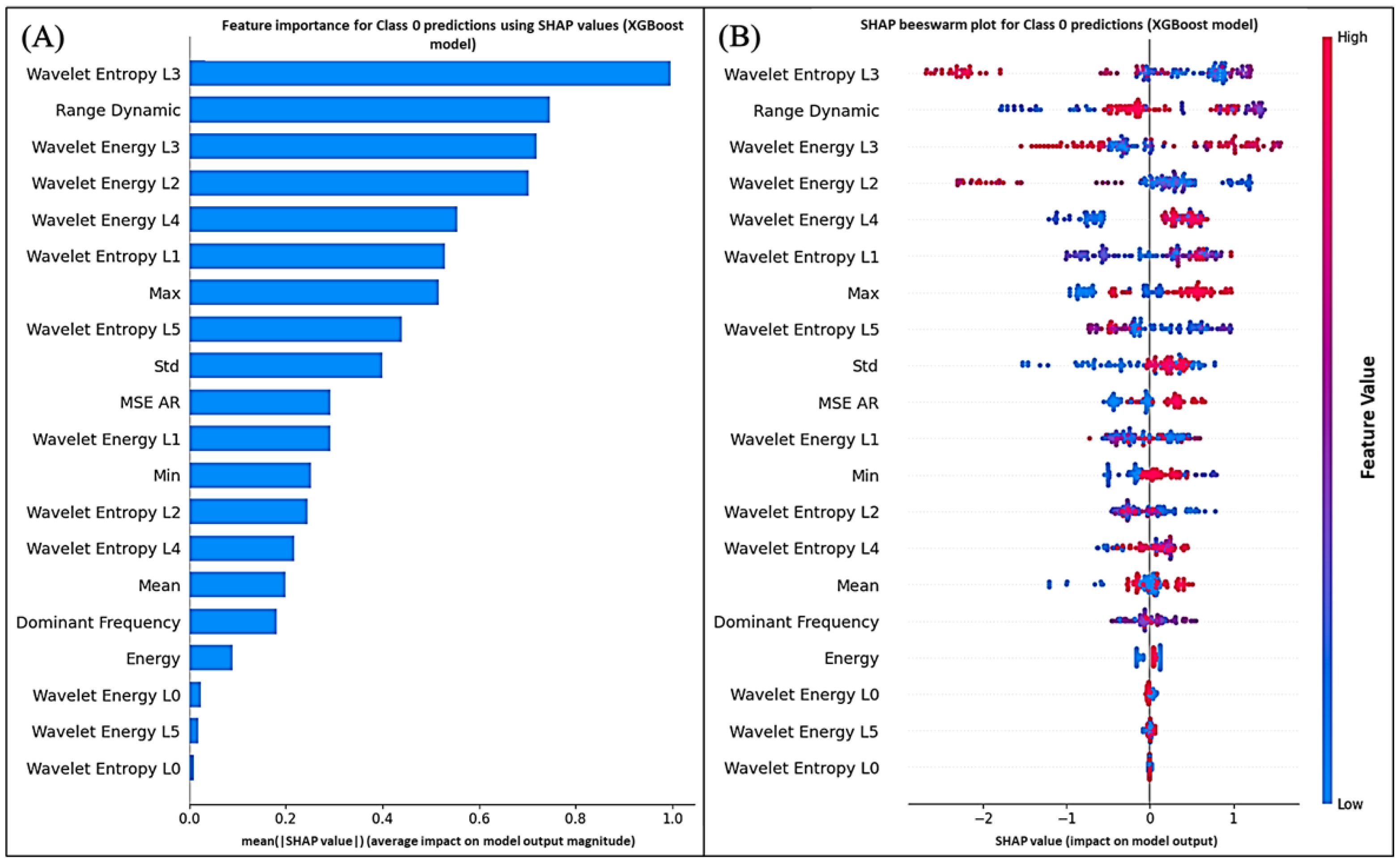
The bootstrap-derived metrics confirm that the XGBoost model is stable, with narrow confidence intervals across all evaluation measures. This indicates that the classifier sustains high performance even under resampling variability, supporting its generalization capability despite the moderate dataset size. However, while these quantitative results show that XGBoost can reliably distinguish between Pb-contaminated and control signals, they do not reveal the basis of its decisions. To address this, SHAP (SHapley Additive exPlanations) analysis was applied to identify the features that most influenced the model’s predictions [23]. This approach links statistical performance with the physiological signal characteristics relevant for classification. Figure 13 and Figure 14 display the global average impact and instance-wise contributions of each feature, respectively.

The SHAP analysis for both Class 1 (polluted) and Class 0 (unpolluted) predictions consistently identified wavelet-based entropy, energy features, and autoregressive (AR) residuals as the main contributors to the model output. These findings support the physiological relevance of the extracted descriptors and align with previous biosensing studies where entropy and wavelet coefficients were among the most predictive features [57].

In particular, mid-level wavelet coefficients (levels 3 and 4) and entropy measures were the most influential features in the SHAP rankings for both classes. Physiologically, these coefficients reflect signal variations over intermediate time windows, linked to ionic fluxes across cell membranes and turgor pressure dynamics. Under Pb stress, disruptions in calcium and potassium homeostasis alter plant electrical potentials, which appear as changes in energy within these frequency bands [6,25,26].

Entropy measures quantify the unpredictability or complexity of the bioelectrical signal. Higher entropy may indicate reduced coordination of electrical activity, potentially linked to membrane damage, altered stomatal function, or impaired phloem transport under heavy metal exposure [58]. The high SHAP importance of entropy features therefore suggests that Pb contamination alters the electrophysiological organization of Aloe vera.

The predominance of mid-level wavelet coefficients and entropy measures in both Class 1 and Class 0 models is consistent with known physiological responses to heavy metal stress. Intermediate frequency components are associated with active transport and vascular signaling in the phloem and xylem, processes that can be disrupted by Pb-induced oxidative stress and ion imbalance. The agreement between SHAP-derived features and established stress physiology supports the biological relevance of the model’s predictions.

Following the SHAP-based interpretation, an additional analysis evaluated whether measurement order influenced the bioelectrical signal patterns. This step aimed to rule out temporal drift or environmental changes during acquisition that might obscure Pb-induced alterations.

To this end, a correlation analysis was performed between the chronological measurement index and key amplitude-related features. Spearman’s rank correlation coefficient ($\rho$) was used, given the non-parametric nature of the data. As shown in

Table 8. Correlation between measurement order and signal amplitude features (Spearman’s $\rho$ and p-value).

Feature	Spearman’s $\mathit{\rho }$	p-Value
Mean amplitude	0.08	0.62
Peak-to-peak value	0.05	0.74
Wavelet level 3 energy	0.09	0.58

, no significant associations were found ($p>0.05$) for mean amplitude, peak-to-peak value, or wavelet level 3 energy. These results indicate that measurement order did not affect the recordings.

The absence of significant correlations supports the robustness of the experimental protocol against temporal bias. However, this analysis cannot replace longitudinal monitoring. Future studies should include repeated measurements across multiple time points for each plant, combined with repeated-measures ANOVA, to better capture intra-plant variability and temporal effects.

This study shows that Pb exposure alters the bioelectrical signals of Aloe vera, but other factors may also affect these signals. Inter-plant variability, electrode placement, and soil moisture can influence amplitude and frequency independently of Pb. To reduce these effects, plants of similar age and size were used, maintained under controlled conditions, with standardized electrode placement and monitored soil moisture. These measures reduced variability but did not eliminate all confounders. Future work should use larger samples, repeated measurements, and explicit modeling of these factors to assess their impact relative to Pb exposure.

Overall, results from classification metrics, SHAP analysis, and correlation tests support the reliability of the proposed approach for detecting Pb stress in Aloe vera. XGBoost showed the best performance, with mid-level wavelet features and entropy measures consistently emerging as key predictors of Pb-related changes. No correlations with measurement order were found, and strict controls reduced the effect of confounding factors. Some limitations remain, including the moderate sample size and natural biological variability. Still, the agreement between statistical, computational, and physiological evidence provides a solid basis for applying this method in environmental biosensing. Future work should use larger datasets, repeated measurements, and validation across species to improve generalization.

4. Conclusions

This study shows that lead (Pb) exposure produces clear and statistically significant changes in the bioelectrical signals of Aloe vera. By combining signal decomposition, autoregressive modeling, and machine learning, it was possible to reliably separate control and Pb-contaminated plants using 160 samples per group. Among the tested classifiers, XGBoost achieved the best accuracy, precision, recall, and F1-score, supported by statistical validation, bootstrap resampling, and SHAP-based interpretability. These results confirm the feasibility of non-invasive electrophysiological monitoring for heavy metal detection and highlight the importance of wavelet-derived features and autoregressive residuals in characterizing contamination-induced stress.

Some limitations remain. Although the sample size is substantial for a controlled electrophysiology study, broader validation with larger and more diverse plant populations under different environmental conditions is needed. Experimental controls reduced the impact of confounding factors such as electrode placement and soil moisture, but these cannot be fully excluded. Future work should include longitudinal monitoring, multi-species validation, and integration with complementary sensing methods to improve accuracy and applicability.

Overall, this work establishes bioelectrical signal analysis as a practical and scalable tool for environmental monitoring. The proposed framework—integrating multiscale analysis, statistical validation, and explainable machine learning—provides a strong basis for the development of field-ready systems for early detection of heavy metal contamination in agricultural and natural ecosystems.

References

1. Frank, J.J.; Poulakos, A.G.; Tornero-Velez, R.; Xue, J. Systematic review and meta-analyses of lead (Pb) concentrations in environmental media (soil, dust, water, food, and air) reported in the United States from 1996 to 2016. Sci. Total Environ. 2019, 694, 133489. [Google Scholar] [CrossRef]
2. Oloruntoba, A.; Omoniyi, A.O.; Shittu, Z.A.; Ajala, R.O.; Kolawole, S.A. Heavy metal contamination in soils, water, and food in Nigeria from 2000–2019: A systematic review on methods, pollution level and policy implications. Water Air Soil Pollut. 2024, 235, 586. [Google Scholar] [CrossRef]
3. World Health Organization (WHO). Lead Poisoning. WHO Fact Sheet, 2024. Available online: https://www.who.int/news-room/fact-sheets/detail/lead-poisoning-and-health (accessed on 15 August 2025).
4. Lanphear, B.P.; Rauch, S.; Auinger, P.; Allen, R.W.; Hornung, R.W. Low-level lead exposure and mortality in US adults: A population-based cohort study. Lancet Public Health 2018, 3, e177–e184. [Google Scholar] [CrossRef]
5. United States Environmental Protection Agency (EPA). EPA Strengthens Safeguards to Protect Families and Children from Lead in Contaminated Soil at Residential Sites in Region 7 (News Release), 17 January 2024. Available online: https://www.epa.gov/newsreleases/epa-strengthens-safeguards-protect-families-and-children-lead-contaminated-soil (accessed on 15 August 2025).
6. Fromm, J.; Lautner, S. Electrical signals and their physiological significance in plants. Plant Cell Environ. 2007, 30, 249–257. [Google Scholar] [CrossRef] [PubMed]
7. Sanderson, B. Note on the electrical phenomena which accompany stimulation of the leaf of Dionaea muscipula. Proc. Roy. Soc. Lond. 1873, 21, 495–496. [Google Scholar] [CrossRef]
8. Volkov, A.G.; Ranatunga, D.R.A. Plants as Environmental Biosensors. Plant Signal. Behav. 2006, 1, 105–115. [Google Scholar] [CrossRef] [PubMed]
9. Shokri, F.; Ziarati, P.; Mousavi, Z. Removal of Selected Heavy Metals from Pharmaceutical Effluent by Aloe vera L. Biomed. Pharmacol. J. 2016, 9, 705–713. [Google Scholar] [CrossRef]
10. Lu, J.; Ding, W. Study and Evaluation of Plant Electrical Signal Processing Methods. In Proceedings of the 4th International Congress on Image and Signal Processing (CISP), Shanghai, China, 15–17 October 2011; pp. 2788–2791. [Google Scholar] [CrossRef]
11. Barbosa-Caro, J.C.; Wudick, M.M. Revisiting plant electric signaling: Challenging an old phenomenon with novel discoveries. Curr. Opin. Plant Biol. 2024, 79, 102528. [Google Scholar] [CrossRef]
12. Chatterjee, S.K.; Das, S.; Maharatna, K.; Masi, E.; Santopolo, L.; Mancuso, S.; Vitaletti, A. Exploring strategies for classification of external stimuli using statistical features of the plant electrical response. J. R. Soc. Interface 2015, 12, 20141225. [Google Scholar] [CrossRef]
13. Yu, K.; Zhang, H.; Zhao, Y. Heavy metal Hg stress detection in tobacco plant using hyperspectral sensing and data-driven machine learning methods. Spectrochim. Acta A Mol. Biomol. Spectrosc. 2021, 245, 118917. [Google Scholar] [CrossRef]
14. Sukhov, V.; Sukhova, E.; Vodeneev, V. Long-distance electrical signals as a link between local action of stressors and systemic physiological responses in higher plants. Prog. Biophys. Mol. Biol. 2019, 146, 63–84. [Google Scholar] [CrossRef]
15. Yang, S.D.; Ali, Z.A.; Kwon, H.; Wong, B.M. Predicting Complex Erosion Profiles in Steam Distribution Headers with Convolutional and Recurrent Neural Networks. Ind. Eng. Chem. Res. 2022, 61, 8520–8529. [Google Scholar] [CrossRef]
16. Geneva, J.; Zabaras, R. Transformers for modeling physical systems. Neural Netw. 2022, 146, 272–289. [Google Scholar] [CrossRef]
17. Zhou, H.; Zhang, S.; Peng, J.; Zhang, S.; Li, J.; Xiong, H.; Zhang, W. Informer: Beyond efficient transformer for long sequence time-series forecasting. Proc. AAAI Conf. Artif. Intell. 2021, 35, 11106–11115. [Google Scholar] [CrossRef]
18. Wu, H.; Xu, J.; Wang, J.; Long, M. Autoformer: Decomposition transformers with auto-correlation for long-term series forecasting. In Advances in Neural Information Processing Systems; Ranzato, M., Beygelzimer, A., Dauphin, Y., Liang, P.S., Wortman Vaughan, J., Eds.; Curran Associates, Inc.: Red Hook, NY, USA, 2021; Volume 34, pp. 22419–22430. [Google Scholar]
19. Alqudah, A.M.; Moussavi, Z. A Review of Deep Learning for Biomedical Signals: Current Applications, Advancements, Future Prospects, Interpretation, and Challenges. Comput. Mater. Contin. 2025, 83, 3753–3841. [Google Scholar] [CrossRef]
20. Yeom, M.S.; Lee, Y.; Oh, H.; Lee, E.; Oh, M.-M. Applying machine learning for the classification of environmental conditions using plant electrical signals. Hortic. Environ. Biotechnol. 2025. [Google Scholar] [CrossRef]
21. Basu, S.K.; Kovalchuk, I. Biosensing with Plants: Plant Receptors for Sensing Environmental Pollution. In Recognition Receptors in Biosensors; Zourob, M., Ed.; Springer: New York, NY, USA, 2010; pp. 263–276. [Google Scholar] [CrossRef]
22. Jana, G.C.; Agrawal, A.; Pattnaik, P.K.; Sain, M. DWT-EMD Feature Level Fusion Based Approach over Multi and Single Channel EEG Signals for Seizure Detection. Diagnostics 2022, 12, 324. [Google Scholar] [CrossRef] [PubMed]
23. Lundberg, S.M.; Lee, S.I. A unified approach to interpreting model predictions. In Proceedings of the 31st International Conference on Neural Information Processing Systems, Long Beach, CA, USA, 4–9 December 2017; Curran Associates Inc.: Red Hook, NY, USA, 2017; pp. 4765–4774. [Google Scholar]
24. Guzmán-Fernández, M.; Zambrano de la Torre, M.; Ortega-Sigala, J.; Guzmán-Valdivia, C.; Galvan-Tejeda, J.I.; Crúz-Domínguez, O.; Ortiz-Hernández, A.; Fraire-Hernández, M.; Sifuentes-Gallardo, C.; Durán-Muñoz, H.A. Arduino: A Novel Solution to the Problem of High-Cost Experimental Equipment in Higher Education. Exp. Tech. 2021, 45, 613–625. [Google Scholar] [CrossRef]
25. Volkov, A.G. Signaling in Electrical Networks of the Venus Flytrap (Dionaea muscipula Ellis). Bioelectrochemistry 2019, 125, 25–32. [Google Scholar] [CrossRef] [PubMed]
26. Sukhova, E.; Sukhov, V. Electrical Signals, Plant Tolerance to Actions of Stressors, and Programmed Cell Death: Is Interaction Possible? Plants 2021, 10, 1704. [Google Scholar] [CrossRef] [PubMed]
27. Chatterjee, S.K.; Malik, O.; Gupta, S. Chemical Sensing Employing Plant Electrical Signal Response—Classification of Stimuli Using Curve Fitting Coefficients as Features. Biosensors 2018, 8, 83. [Google Scholar] [CrossRef] [PubMed]
28. Hardstone, R.; Poil, S.-S.; Schiavone, G.; Jansen, R.; Nikulin, V.V.; Mansvelder, H.D.; Linkenkaer-Hansen, K. Detrended fluctuation analysis: A scale-free view on neuronal oscillations. Front. Physiol. 2012, 3, 450. [Google Scholar] [CrossRef]
29. Huang, N.E.; Shen, Z.; Long, S.R.; Wu, M.C.; Shih, H.H.; Zheng, Q.; Yen, N.C.; Tung, C.C.; Liu, H.H. The empirical mode decomposition and the Hilbert spectrum for nonlinear and non-stationary time series analysis. Proc. R. Soc. Lond. A 1998, 454, 903–995. [Google Scholar] [CrossRef]
30. Chen, Y.; Zhao, D.-J.; Wang, Z.-Y.; Tang, G.; Huang, L. Plant Electrical Signal Classification Based on Waveform Similarity. Algorithms 2016, 9, 70. [Google Scholar] [CrossRef]
31. Torre, M.Z.-d.l.; Sifuentes-Gallardo, C.; González-Ramírez, E.; Cruz-Dominguez, O.; Ortega-Sigala, J.; Díaz-Flórez, G.; Vargas, J.I.D.l.R.; Durán-Muñoz, H. Electrical Signal Characterization of Aloe vera Var. Chinensis Using Non-Parametric and Parametric Signal Analysis. Appl. Sci. 2025, 15, 1708. [Google Scholar] [CrossRef]
32. Bandt, C.; Pompe, B. Permutation entropy: A natural complexity measure for time series. Phys. Rev. Lett. 2002, 88, 174102. [Google Scholar] [CrossRef] [PubMed]
33. Zanin, M.; Zunino, L.; Rosso, O.A.; Papo, D. Permutation Entropy and Its Main Biomedical and Econophysics Applications: A Review. Entropy 2012, 14, 1553–1577. [Google Scholar] [CrossRef]
34. Chen, Z.; Ivanov, P.C.; Hu, K.; Stanley, H.E. Effect of Nonstationarities on Detrended Fluctuation Analysis. Phys. Rev. E 2002, 65, 041107. [Google Scholar] [CrossRef]
35. Cortes, C.; Vapnik, V. Support-vector networks. Mach. Learn. 1995, 20, 273–297. [Google Scholar] [CrossRef]
36. Breiman, L. Random Forests. Mach. Learn. 2001, 45, 5–32. [Google Scholar] [CrossRef]
37. Chen, T.; Guestrin, C. XGBoost: A scalable tree boosting system. In Proceedings of the 22nd ACM SIGKDD Conference, San Francisco, CA, USA, 13–17 August 2016; pp. 785–794. [Google Scholar] [CrossRef]
38. Suthaharan, S. Support Vector Machine. In Machine Learning Models and Algorithms for Big Data Classification; Springer: Boston, MA, USA, 2016; Volume 36, pp. 207–235. [Google Scholar] [CrossRef]
39. M’hamdi, O.; Takács, S.; Palotás, G.; Ilahy, R.; Helyes, L.; Pék, Z. A comparative analysis of XGBoost and neural network models for predicting some tomato fruit quality traits from Environmental and Meteorological Data. Plants 2024, 13, 746. [Google Scholar] [CrossRef] [PubMed]
40. Wang, L.; Li, H.; Li, D.; Zhao, J. A Prediction on Electric Signals Processing of Aloe vera var. Chinensis. In Proceedings of the Third International Conference on Natural Computation (ICNC 2007), Haikou, China, 24–27 August 2007; pp. 90–94. [Google Scholar] [CrossRef]
41. Kumar, S.; Trivedi, P.K. Heavy Metal Stress Signaling in Plants. In Plant Metal Interaction; Ahmad, P., Ed.; Elsevier: Amsterdam, The Netherlands, 2016; pp. 585–603. [Google Scholar] [CrossRef]
42. Zhou, J.; Yuan, W.; Di, B.; Zhang, G.; Zhu, J.; Zhou, P.; Ding, T.; Qian, J. Relationship among electrical signals, chlorophyll fluorescence, and root vitality of strawberry seedlings under drought stress. Agronomy 2022, 12, 1428. [Google Scholar] [CrossRef]
43. Broock, W.A.; Scheinkman, J.A.; Dechert, W.D.; LeBaron, B. A Test for Independence Based on the Correlation Dimension. Econom. Rev. 1996, 15, 197–235. [Google Scholar] [CrossRef]
44. Yu, X. ECG Signal Classification Based on DWT Denoising and XGBoost. Appl. Comput. Eng. 2024, 95, 57–67. [Google Scholar] [CrossRef]
45. Sai, K.; Sood, N.; Saini, I. Abiotic Stress Classification through Spectral Analysis of Enhanced Electrophysiological Signals of Plants. Biosyst. Eng. 2022, 219, 189–204. [Google Scholar] [CrossRef]
46. Kumari, A.; Edla, D.R. Integrated EMD-Enhanced Analysis and Neural Network Classification for Robust Processing of Motor Imagery EEG Signals. Procedia Comput. Sci. 2025, 258, 2018–2028. [Google Scholar] [CrossRef]
47. Mudrilov, M.; Ladeynova, M.; Grinberg, M.; Balalaeva, I.; Vodeneev, V. Electrical Signaling of Plants under Abiotic Stressors: Transmission of Stimulus-Specific Information. Int. J. Mol. Sci. 2021, 22, 10715. [Google Scholar] [CrossRef]
48. Jovanov, E.; Milenkovic, A.; Otto, C.; de Groen, P. A wireless body area network of intelligent motion sensors for computer assisted physical rehabilitation. J. NeuroEng. Rehabil. 2005, 2, 6. [Google Scholar] [CrossRef] [PubMed]
49. Gao, W.; Xiao, T.; Zou, L.; Li, H.; Gu, S. Analysis and Prediction of Atmospheric Environmental Quality Based on the Autoregressive Integrated Moving Average Model (ARIMA Model) in Hunan Province, China. Sustainability 2024, 16, 8471. [Google Scholar] [CrossRef]
50. Figueiredo, E.; Figueiras, J.; Park, G.; Farrar, C.R.; Worden, K. Influence of the Autoregressive Model Order on Damage Detection. Comput.-Aided Civ. Infrastruct. Eng. 2011, 26, 225–238. [Google Scholar] [CrossRef]
51. Li, P.; Wang, X.; Li, F.; Zhang, R.; Ma, T.; Peng, Y.; Lei, X.; Tian, Y.; Guo, D.; Liu, T.; et al. Autoregressive Model in the Lp Norm Space for EEG Analysis. J. Neurosci. Methods 2015, 240, 170–178. [Google Scholar] [CrossRef] [PubMed]
52. Lysov, M.; Maximova, I.; Vasiliev, E.; Getmanskaya, A.; Turlapov, V. Entropy as a High-Level Feature for XAI-Based Early Plant Stress Detection. Entropy 2022, 24, 1597. [Google Scholar] [CrossRef] [PubMed]
53. Rafiee, J.; Rafiee, M.A.; Prause, N.; Schoen, M.P. Wavelet Basis Functions in Biomedical Signal Processing. Expert Syst. Appl. 2011, 38, 6190–6201. [Google Scholar] [CrossRef]
54. Li, Y.-X.; Jiao, S.-B.; Gao, X. A Novel Signal Feature Extraction Technology Based on Empirical Wavelet Transform and Reverse Dispersion Entropy. Def. Technol. 2021, 17, 1625–1635. [Google Scholar] [CrossRef]
55. Coulibaly, S.; Kamsu-Foguem, B.; Kamissoko, D.; Traore, D. Deep Learning for Precision Agriculture: A Bibliometric Analysis. Intell. Syst. Appl. 2022, 16, 200102. [Google Scholar] [CrossRef]
56. Gokgoz, E.; Subasi, A. Comparison of Decision Tree Algorithms for EMG Signal Classification Using DWT. Biomed. Signal Process. Control 2015, 18, 138–144. [Google Scholar] [CrossRef]
57. Ponce-Bobadilla, A.V.; Schmitt, V.; Maier, C.S.; Mensing, S.; Stodtmann, S. Practical Guide to SHAP Analysis: Explaining Supervised Machine Learning Model Predictions in Drug Development. Clin. Transl. Sci. 2024, 17, e70056. [Google Scholar] [CrossRef]
58. Vitelli, V.; Giamborino, A.; Bertolini, A.; Saba, A.; Andreucci, A. Cadmium Stress Signaling Pathways in Plants: Molecular Responses and Mechanisms. Curr. Issues Mol. Biol. 2024, 46, 6052–6068. [Google Scholar] [CrossRef]
Figure 1. Methodology (stages 1–8) implemented for the development of the lead presence detector through the analysis of the electrical signal from the Aloe vera plant.
Applsci 15 09319 g001
Figure 2. Graphic description of the lead contamination process on the Aloe vera plant. (A) Lead concentration. (B) Surgical-grade lead supply line. (C) Electronic measuring equipment. (D) Aloe vera.
Applsci 15 09319 g002
Figure 3. Implementation of the electrode insertion technique. (A) Aloe vera plant and (B) stainless steel electrodes.
Applsci 15 09319 g003
Figure 4. General schematic of the electronic array. Capital letters (A–I) correspond to labels in the figure: (A) DHT11, (B) ATMega328P, (C) LDR photoresistor module, (D) FC-28 soil moisture module, (E) stainless steel electrodes, (F) LM324, (G) Aloe vera, (H) pair of soil moisture probes, and (I) MicroSD memory module.
Applsci 15 09319 g004
Figure 5. (A) Electrical signal of uncontaminated Aloe vera and (B) electrical signal contaminated with lead.
Applsci 15 09319 g005
Figure 6. (A) Box plot and (B) density plot of the signal response with and without lead.
Applsci 15 09319 g006
Figure 7. Autocorrelation analysis of the Aloe vera bioelectrical signal. The function R x ( τ ) is plotted against discrete time lags (sampling rate: 10 Hz). The orange line with markers corresponds to the autocorrelation values, while the pink horizontal line indicates the zero reference level. Correlations decay rapidly within the first few lags, indicating a short memory period followed by random-like behavior.
Applsci 15 09319 g007
Figure 8. DFA log–log plot showing the fluctuation function F ( s ) as a function of window size s for control and Pb-contaminated Aloe vera signals.
Applsci 15 09319 g008
Figure 9. Three-dimensional DWT decomposition of the Aloe vera signal (db3, five levels). The black trace shows the Pb-contaminated signal and the blue lines are the wavelet decomposition levels.
Applsci 15 09319 g009
Figure 10. Energy (top) and Shannon entropy (bottom) for each IMF extracted via EMD. Mid-range IMFs exhibit the highest complexity, while the first IMF captures most of the signal’s energy.
Applsci 15 09319 g010
Figure 11. AR(10) reconstruction of the lead-contaminated Aloe vera electrical signal. The red line shows the model prediction closely following the original signal (dashed line).
Applsci 15 09319 g011
Figure 12. Confusion matrices for the classification algorithms: (A) SVM, (B) XGBoost, and (C) Random Forest. The intensity of the blue color indicates the number of instances, with darker shades representing higher counts.
Applsci 15 09319 g012
Figure 13. SHAP analysis of Class 1 (polluted) predictions with XGBoost. (A) Feature ranking by mean absolute SHAP values. (B) Beeswarm plot showing feature contributions per instance (red = high, blue = low).
Applsci 15 09319 g013
Figure 14. SHAP analysis of Class 0 (unpolluted) predictions with XGBoost. (A) Feature ranking by mean absolute SHAP values. (B) Beeswarm plot showing feature contributions per instance (red = high, blue = low).
Applsci 15 09319 g014