Featured Application
Our research offers practical solutions with direct real-world applicability: (1) Intersection-Level Optimization: We propose a novel signal control method that addresses three critical yet overlooked challenges in existing studies: (1) impact of pedestrian stages and overlap phases on signal optimization models, (2) coupling effects of signal cycles and queue lengths, and (3) stochastic vehicle arrivals in undersaturated conditions. (2) Deployable System Architecture: A cloud–edge–terminal framework has been implemented in real-world settings (with equipment brands detailed in the paper). The cloud platform provides traffic managers with an interactive interface for system monitoring and control. (3) Validation Platform: Our hardware-in-the-loop simulation system has supported multiple editions of the Shanghai Intelligent New Energy Vehicle Big Data Competition. (4) Field Results: Real-world tests on Chengaodadao, Conghua District, Guangzhou, China demonstrate a 50% reduction in stops and 27% shorter travel times in coordinated directions.
Abstract
Coordinated adaptive signal control is a proven strategy for improving traffic efficiency and minimizing vehicular delays. First, we develop a Queue Evolution and Delay Model (QEDM) that establishes the relationship between detector-measured queue lengths and model parameters. QEDM accurately characterizes residual queue dynamics (accumulation and dissipation), significantly enhancing delay estimation accuracy under oversaturated conditions. Secondly, we propose a novel intersection-level signal optimization method that addresses key practical challenges: (1) pedestrian stages, overlap phases; (2) coupling effects between signal cycle and queue length; and (3) stochastic vehicle arrivals in undersaturated conditions. Unlike conventional approaches, this method proactively shortens signal cycles to reduce queues while avoiding suboptimal solutions that artificially “dilute” delays by extending cycles. Thirdly, we introduce an adaptive coordination control framework that maintains arterial-level green-band progression while maximizing intersection-level adaptive optimization flexibility. To bridge theory and practice, we design a cloud–edge–terminal collaborative deployment architecture for scalable signal control implementation and validate the framework through a hardware-in-the-loop simulation platform. Case studies in real-world scenarios demonstrate that the proposed method outperforms existing benchmarks in delay estimation accuracy, average vehicle delay, and travel time in coordinated directions. Additionally, we analyze the influence of coordination constraint update intervals on system performance, providing actionable insights for adaptive control systems.
1. Introduction
With the rapid development of science, technology, and industry, cities are expanding in both population and area. Production and daily life are becoming more concentrated. However, as motorization progresses, demand for urban transportation continues to outstrip available capacity—INRIX’s 2024 Global Traffic Scorecard reports drivers in major cities like Istanbul, New York City, Chicago, and London losing over 100 h per year to congestion, with delays costing the U.S. economy more than USD 74 billion in 2024 [1]. According to the International Energy Agency, in 2024 the transport sector consumed over one-quarter of global final energy—more than 90% from oil products—and emitted about 8 Gt of CO2, with road transport emissions projected to peak at around 9 Gt in 2025; a substantial share of this energy use and emissions stems from urban traffic congestion, where idling and stop-and-go conditions significantly increase fuel consumption and pollutant output [2]. Signalized intersections, serving as key points where traffic flows converge, often become bottlenecks within urban traffic networks [3]. On many occasions, the causes of congestion are not necessarily attributable to road infrastructures themselves. Instead, the existing signal control systems excessively rely on the use of IT technology but ignore the basic theory of traffic control and the essential consideration of the traffic environment and optimal regulation of road traffic flow, which greatly limits the scientific and practical value of traffic control systems [4].
According to the current situation with urban traffic control systems, signal control strategies can be divided into fixed-time control, actuated control, and adaptive signal control for isolated intersections and coordinated control for arterials [5]. Webster proposed one of the earliest fixed-time control models to minimize the average delay per vehicle, which builds a foundation for modeling and optimizing the traffic signals of isolated intersections. Empirical data were developed from previous research tasks and from field studies at three intersections in the London area to validate results and calibrate the variables [6]. However, fixed timing plans need to be updated and optimized for the current traffic demand. Outdated or poorly timed fixed-time signal plans can lead to additional traffic delays and congestion [7]. Compared to fixed-time, actuated control can be responsive to time-dependent dynamic traffic demand. However, introduction of control variables, such as minimum green time, maximum green time, and green time extension increment, contributes to system operational flexibility and complexity. As a downside, the complicated nature of actuated control operation gives rise to a lot of uncertainties and unexpected results in the system, so that practical engineers and signal designers find it difficult to make full utilization of the potential benefits of actuated signals [8,9].
In the field of adaptive control, early delay studies did not incorporate queue length as an input [6]. As demonstrated in SCATS (Sydney Coordinated Adaptive Traffic System), headway-based demand estimation loses accuracy when residual queues persist into subsequent cycles, impairing adaptive traffic control performance. Research has primarily concentrated on the formulation of optimization objectives [10,11] and the development of solution methods [12]. Wang et al. conducted an evaluation of control delay estimation methods and indicated that the HCM 2000 model performs satisfactorily under various v/c ratios, while the deterministic queuing model has better performance when the v/c ratio is extremely high [13]. With growing recognition that both volume and queue length are essential to accurately reflect real demand [14], recent studies have started to include queue length in the modeling process. They have focused on various aspects such as isolated adaptive signal control [15,16], coordinated adaptive control [17], integrated optimization of adaptive control and lane allocation [18], and adaptive signal control in connected vehicle (CV) environments [19]. However, although these studies have incorporated queue length into delay estimation models, the accuracy remains limited, as queue-related metrics are primarily derived from license plate recognition (LPR) data [20] or vehicle trajectory data [21]. Moreover, it is challenging to establish a clear correspondence between the queue length estimated in the real world and parameters within mathematical models. With the development of multimodal object detection techniques [22,23], multi-sensor fusion devices (MSFDs) combining radar and camera inputs have demonstrated the capability to accurately detect vehicle position, velocity, and heading [24]. This facilitates precise identification of queue length, thereby effectively overcoming the limitations of earlier methods that relied on indirect inference of queue length.
The optimization objectives for coordinated signal control are generally divided into two categories: bandwidth maximization and performance indicator optimization [17,25]. Bandwidth maximization offers a clear physical interpretation of the optimization results, and its associated models are relatively simple and highly scalable, leading to widespread adoption [26]. Representative methods include MaxBand [27], MultiBand [28], and AMBand [29]. However, in the context of coordinated adaptive control, limited research has been conducted on the interaction mechanisms between arterial-level coordination and intersection-level adaptive control. This gap restricts the ability of coordinated adaptive control to effectively respond to dynamic traffic demand. Wang et al. first performed intersection-level optimization, and then optimized offsets based on it. A simulation based on a real-world arterial showed that the proposed control system could be applied in the field to boost the overall traffic efficiency along the arterial [25], but this optimization framework limits the frequency of intersection-level optimization. Hao et al. constrained the probability that the green splits of the coordinated phase in intersection-level optimization are greater than or equal to the required green splits from arterial-level optimization. The results showed that the proposed model can effectively reduce the average intersection delay and the average residual queue length compared with Webster’s method and Allsop’s method [30]. Beak et al. constrained the minimum and maximum green times of the coordinated phase in intersection-level optimization from the initial split in arterial-level optimization. The results indicated that the model could reduce average delay and average number of stops for both coordinated routes and the entire network [31]. If the coordinated phase is not the leading phase, imposing constraints only on its green time duration may not prevent local adaptive strategies from disrupting the green band progression. Ma et al. constrained the green splits of the coordinated phases to only be extended to maintain a minimum through-band, while the green splits of non-coordinated phases could be decreased [17]. Although this approach preserved the green band progression, it excessively restricted the flexibility of isolated optimization.
To summarize, the existing literature has proposed many optimization strategies for delay estimation and coordinated adaptive control, but there is still room for improvement:
- (1)
- To address the issue of insufficient delay estimation accuracy, existing studies often rely on indirectly derived queue lengths from detection data, which introduces estimation errors. Moreover, the relationship between queue length and delay model parameters remains unclear, resulting in limited accuracy in delay estimation. To overcome these limitations, this study introduces a Multi-Sensor Fusion Device (MSFD) to directly detect queue length, thereby eliminating estimation errors. Based on this, a novel delay estimation model is developed, which explicitly defines the relationship between queue length and model parameters. The proposed model accurately captures the dissipation and accumulation dynamics of residual queues, significantly improving delay estimation accuracy under oversaturated conditions.
- (2)
- A new intersection-level optimization method is proposed that considers multiple elements, such as pedestrian phases, overlap phases, the coupling effects of signal schemes and queue lengths, and the stochastic characteristics of vehicle arrivals in the unsaturated state. This method can proactively reduce the cycle to decrease queue lengths and prevent the optimization results from selecting large cycle to “dilute” the average vehicle delay.
- (3)
- Regarding the lack of coordination between optimization layers in adaptive coordinated control, existing approaches often face conflicts between intersection-level and arterial-level constraints, making it difficult to balance local and global performance. To tackle this challenge, this study proposes a new adaptive coordination control framework that preserves the green band progression at the arterial level while fully leveraging the optimization potential of adaptive optimization at the intersection level. The framework offers high compatibility and can be integrated with various coordination and adaptive optimization algorithms.
- (4)
- As for the insufficient consideration of deployment details in coordinated adaptive control, current theoretical studies often overlook key factors such as adaptive update intervals, pedestrian stages, overlapping phases, and signal transition times, which hinders practical implementation. This study systematically incorporates these deployment-related factors into the theoretical modeling process and develops a cloud–edge–terminal collaborative deployment architecture and an in-the-loop simulation platform to facilitate the real-world application of coordinated adaptive control.
2. Methodology
2.1. Queue Evolution and Delay Model
2.1.1. Green Start and Red Start Queued Vehicles
Denote the cycle duration of the cycle as , the effective green duration of phase as , and the red duration as . The number of lanes and average saturation flow rate for phase are and , respectively. The average vehicle arrival rate and maximum queue length detected by MSFD for phase are and , respectively. The number of queued vehicles at the start of green for phase in cycle is calculated as , where and represent the average vehicle length and minimum safe space, respectively. The number of queued vehicles at the start of red (red start) for phase in cycle is .
In existing studies [17,18], to simplify model formulation, the red start queue length is assumed to be known, and the green start queue length is derived as: . However, detecting the red start queue length requires identifying the initial moment of the red phase using SPAT (Signal Phase And Timing) messages from a signal controller, which cannot be achieved solely through MSFD. In contrast, the green start queue length can be accurately calculated using the maximum queue length directly output by MSFD combined with the average vehicle length and minimum safe spacing. Moreover, in real-world scenarios when the red start queue length is zero, the green start queue length may be greater than zero (if vehicles arrive during the red phase) or equal to zero (if no vehicles arrive during the red phase). Existing studies can only describe the former case and fail to capture the latter phenomenon.
2.1.2. Queue Delay Model (QDM)
The queue clearance time for phase in cycle is . In an undersaturated state, the queue clears within effective green time, i.e., . An oversaturated state is otherwise, as shown in Figure 1.
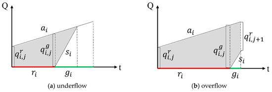
Figure 1.
Undersaturated and Saturated States.
Total delay for phase in cycle in an undersaturated state is the sum of the shaded trapezoidal area during red and the shaded triangular area during green:
Total delay for phase in cycle in an oversaturated state is the difference between the trapezoidal area over the entire cycle and the unshaded triangular area during green:
Average vehicle delay for phase in cycle equals the total vehicle delay divided by the total number of vehicles:
2.1.3. Queue Evolution Delay Model (QEDM)
Existing studies [17,18] calculate delays solely based on the undersaturated/oversaturated states shown in Figure 1. However, under oversaturated conditions (Figure 1b), residual queued vehicles from cycle significantly impact delays in cycle . In Figure 2a, residual queues accumulate progressively across cycles, causing shaded delay areas to expand. This may lead to queue spillback to upstream intersections, potentially paralyzing the network. In Figure 2b, residual queues gradually dissipate, eventually transitioning to the undersaturated state in Figure 1a. To reflect real-world oversaturated delays, delay calculations must account for multi-cycle cumulative effects of queue evolution as shown in Figure 2.
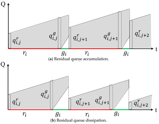
Figure 2.
Residual Queue Accumulation and Dissipation Across Cycles.
Red-start queued vehicles for phase in cycle is the residual queue from cycle : . Green-start queued vehicles for phase in cycle : . The arrival rate is used instead of because only MSFD detection data from cycle are available. Queue evolution is thus calculated using cycle ’s data. Number of cycles required for the tail of cycle ’s green-start queue to clear the intersection , where denotes the ceiling function (rounding up). To characterize queue evolution in oversaturated states, the aggregate average vehicle delay over cycles from cycle must be calculated:
2.2. Intersection-Level Optimization Based on QEDM
To accommodate time-varying traffic demands of various directions and pedestrian crossings, complex phase schemes often include overlapping phases and dedicated pedestrian stages, as illustrated in Figure 3. Stage D is the pedestrian stage where green time = 0, yellow time = 0, and all-red time = 28 s. In other phases, yellow time = 3 s and all-red time = 0 s. Phase 1 is the overlapping phase for Stage A and Stage B. Phase 3 is the overlapping phase for Stage B and Stage C.
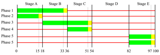
Figure 3.
Diagram Illustrating the Association Between Phases and Stages.
Under complex phase scheme design, the effective green time calculation for phase is:
where represents the relationship between phase and stage . If stage allows phase to pass, then = 1, otherwise = 0. represents the green time for stage in cycle and and represent yellow and all-red times for stage . is the loss time. When , phase is the overlapping phase for stage and . After combination with stage , no signal transition occurred in phase , so all-red time counts toward effective green and there is no need to subtract the signal loss time. When and , signal transition occurs in phase . All-red time is excluded from effective green and signal loss time needs to be subtracted.
The intersection-level optimization objective is to compute optimal green time for all stages at each intersection in real time to achieve control goals while satisfying constraints. The model is usually shown as P1-1.
(P1-1):
Objective function:
Constraints include (4), (5), (6), and
The objective function (7) minimizes the average vehicle delay at the intersection. Constraint (6) computes the effective green time for each phase considering overlapping phases and pedestrian stages. Constraints (4) and (5) calculate phase-specific delays using the Queue Evolution and Delay Model (QEDM). Constraint (8) defines the relationship between stage green times, yellow times, all-red times, and cycle length. Constraints (9) and (10) set upper/lower bounds for stage green times and cycle length. Constraint (11) limits the maximum saturation degree for all phases.
Existing studies fail to describe the relationship between queue length and delay model parameters; thus, the impact of signal settings on initial green-start queues is not considered, which leads to models only responding to longer queues by passively increasing cycle length but lacking mechanisms to proactively decrease cycle length for queue reduction. Denote the actual green-start queue as and actual red-start queue as , where is the actual red duration for phase in cycle . The relationship between stage green times and phase green-start queues in the optimization scheme is formalized as:
In Equation (12), the actual red-start queue represents residual vehicles from the previous cycle and is unaffected by planned timing schemes. The planned green-start queue is derived from the planned red duration . Equation (13) quantifies the impact of planned timing on green-start queues. Equal red durations: Planned queue = actual queue. Longer planned red time: Planned queue > actual queue, reflecting increased queues due to extended cycle. Shorter planned red time: Planned queue < actual queue. The green-start queue is corrected as the weighted average of planned and actual queue, reflecting the potential for shorter planned cycles to reduce queue length and prevent short planned cycles from failing to clear the actual green-start queue.
Existing studies [6,10,17], as in Equation (3), typically assume a positive correlation between the number of arrivals in a cycle and the cycle length. This assumption often causes optimization results to favor longer cycle lengths, in order to “dilute” average vehicle delay and thereby achieve the objective of minimizing average vehicle delay. Denote the actual saturation for phase in cycle as , where and represent actual cycle length and effective green time for phase . When the actual saturation is low, i.e., , vehicle arrivals can be considered discrete. In this case, changes in cycle length will not affect the total number of arrivals within the cycle. Accordingly, Equation (4) should be revised as:
In Equation (14), when the actual saturation of phase is low, the average vehicle delay is calculated based on the actual number of vehicles arriving within the cycle. When the actual saturation of phase is high, the average vehicle delay is calculated using the planned number of vehicle arrivals within the cycle. Based on model P1-1, and incorporating the improvements made in Equations (12)–(14), an intersection-level hierarchical optimization model P1-2 is established:
(P1-2):
Objective function: (7)
Constraints: (5), (6), (8)–(14)
Where the objective function (7) and the constraints (5), (6), (8)–(10) are the same as those in model P1-1. Constraint (14) prevents the optimization results from tending toward the selection of long cycle lengths to “dilute” the average vehicle delay. Constraints (11) and (12) describe the influence of the planned signal timing scheme on the queue length at the start of the green phase.
2.3. Arterial-Level Optimization
Classic arterial-level coordination optimization methods include MaxBand [27], MultiBand [28], and AMBand [29]. Taking MaxBand as an example, the relevant parameters involved in the model are illustrated in Figure 4.
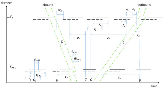
Figure 4.
Schematic diagram of the MaxBand model.
(P2-1):
Objective function:
Constraints:
where denotes outbound (inbound) bandwidth ratio, denotes red time (cycles) of coordinated phase of outbound (inbound), and denotes time from right (left) side of red at intersection to left (right) edge of outbound (inbound) green band. denotes intranode offset, which is the time difference between the center of and the nearest center of . It is positive if the center of is to the right of the center of . denotes outbound (inbound) distance between intersection and intersection , denotes outbound (inbound) travel time (cycles) between intersection and intersection , and denotes outbound (inbound) travel speed. denotes outbound (inbound) queue clearance time (cycles) at intersection .
MaxBandtakes the red time in the coordinated direction at each intersection as a parameter and aims to maximize the bidirectional weighted bandwidth ratio, solving for the optimal , . The cycle length is constrained by the range , . However, if and are set inappropriately, they may lead to unreasonable cycle lengths at certain intersections, resulting in empty green times or oversaturation. Therefore, an additional constraint on the cycle length range is introduced, leading to the establishment of model P2-2.
(P2-2):
Objective function: (15)
Constraints: (16)–(24), and
where denotes the optimal cycle length of intersection obtained from model P1-2, and represents the adjustment range for the cycle length in coordination optimization.
2.4. Coordinated Adaptive Control Framework
In existing studies [17,25,30,31], the interaction between arterial-level coordination and intersection-level adaptive control has been insufficiently addressed. Wang et al. first performed intersection-level optimization, and then optimized offsets based on it, although this framework limits the frequency of intersection-level optimization [25].
On the one hand, if the adaptive optimization range at intersections is too large, it disrupts the coordinated green band along the arterial. Hao et al. constrained the probability that the green splits of the coordinated phase in intersection-level optimization are greater than or equal to the required green splits from arterial-level optimization [30]. Beak et al. constrained the minimum and maximum green times of the coordinated phase in intersection-level optimization from the initial split in arterial-level optimization [31]. If the coordinated phase is not the leading phase, imposing constraints only on its green time duration may not prevent local adaptive strategies from disrupting the green band progression.
On the other hand, if the optimization range is overly restricted to maintain the green band, the intersection’s adaptive functionality is nearly disabled. Ma et al. constrained the green splits of the coordinated phases to only be extended to maintain a minimum through-band, while the green splits of non-coordinated phases could be decreased [17]. Although this approach preserved the green band progression, it excessively restricted the flexibility of isolated optimization.
This study proposes a new adaptive coordination control framework that preserves green band progression at the arterial level while fully leveraging the optimization potential of adaptive control at the intersection level. A comparison of the proposed framework and benchmarks is presented in Table 1. Overall, Wang’s framework does not support high-frequency intersection-level optimization and thus cannot be considered adaptive coordinated control. Hao’s and Beak’s frameworks do not support lagging coordinated phases, making them unable to preserve green band progression. Additionally, the frameworks of Hao, Beak, and Ma do not allow shortening of the coordinated phase, resulting in an overly restricted optimization range at the intersection level.

Table 1.
Comparison of different frameworks.
At the coordination control level, a 30 min or longer update interval is used. Average traffic demand over this period at each intersection serves as the data source. Model P1-2 is used to determine the optimal green time for each stage at each intersection, as well as the optimal cycle length . Based on Equation (6), the effective green time of the coordinated phase is calculated. The proportion of red time in the cycle for the coordinated direction is computed as , . By substituting into model P2-2, the optimal common cycle length for coordination and the optimal offsets for each intersection are obtained. The optimal green time for stage at intersection is then given by:
To preserve the green band progression at the arterial level while fully leveraging the optimization potential of adaptive optimization at the intersection level, let the left and right boundaries of the outbound (inbound) green band at a given intersection be denoted by and , respectively.
Let the outbound coordinated phase be denoted as , then the set of outbound coordinated stages is . The first outbound coordinated stage is . The last outbound coordinated stage is . Similarly, the first and last inbound coordinated stages, denoted and , can be obtained in the same way. By adding coordination scheme constraints based on these definitions, model P1-3 is established.
(P1-3):
Objective function: (7)
Constraints: (5), (6), (8)–(14), and:
As shown in Figure 5, constraints (29) and (31) ensure that the start time of the coordinated phase in the adaptive plan is no later than the left boundary of the green band in the coordination scheme; constraints (30) and (32) ensure that the end time of the coordinated phase in the adaptive plan is no earlier than the right boundary of the green band. Constraint (33) ensures that the cycle length of the intersection-level adaptive plan is consistent with the common cycle length.
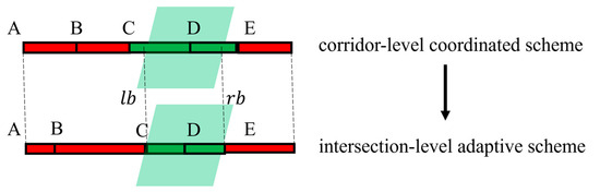
Figure 5.
Coordination Scheme Constraints.
As illustrated in Figure 6, models P1-2, P2-2, and P1-3 together form the coordinated adaptive optimization framework. Among them, P1-2 and P2-2 are responsible for low-frequency (e.g., every 30 min) optimization at the arterial level, generating a coordinated scheme that includes a common cycle length and green band widths adapted to long-term average traffic demand. This coordination of constraints and offsets is passed to the intersection-level adaptive optimizer. The P1-3 model performs high-frequency optimization (e.g., every 5 min) at the intersection level, enabling real-time adjustment of green times for each stage according to short-term traffic demand. It is important to note that the coordinated adaptive optimization framework proposed in this study is compatible with various types of adaptive and coordination control algorithms. One only needs to replace the models in the three steps: corridor-1, corridor-2, and intersection-1. The coordination constraints, i.e., Equations (29)–(33) derived from arterial-2, are then passed into intersection-1 for further optimization.
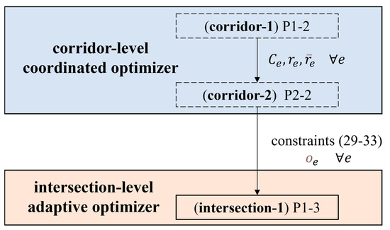
Figure 6.
Coordinated Adaptive Optimization Framework.
3. Deployment
3.1. Overall Architecture
Figure 7 illustrates a cloud–edge–terminal collaborative architecture for coordinated adaptive traffic signal control, designed to bridge the gap between theoretical research and practical engineering applications. This three-tiered system enables both large-scale coordination and real-time adaptive control through distributed computing.
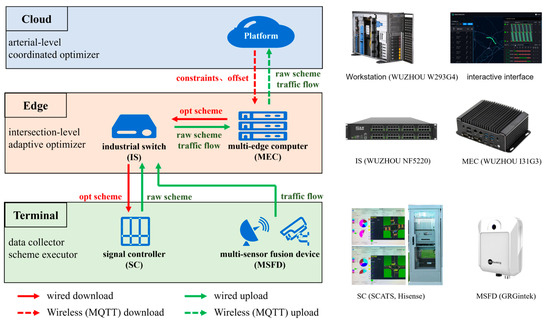
Figure 7.
Cloud–Edge–Terminal Collaborative Deployment Architecture for Coordinated Adaptive Signal Control.
At the cloud level, deployed in the control center, the corridor-level coordinated optimizer performs low-frequency optimization (typically every 30 min) to maintain arterial coordination and green wave bands. The cloud platform subscribes to data from edge devices and publishes coordination constraints (including offsets and cycle parameters) back to them using MQTT wireless communication. A user interface at this level allows for system monitoring and manual intervention when needed.
The edge layer, deployed roadside, consists of multiple edge computing nodes (MECs) that handle high-frequency, intersection-level adaptive optimization (typically every 5 min). These MECs receive both real-time traffic data from terminal devices and coordination constraints from the cloud, enabling them to optimize individual intersections while maintaining arterial coordination. An industrial switch facilitates high-speed wired communication between edge devices and terminal equipment.
At the terminal level, various devices interface directly with the physical infrastructure. Traffic signal controllers (including SCATS and Hisense models) execute optimized signal plans while reporting current status. Multi-sensor fusion devices (MSFDs) collect and process real-time traffic flow data from multiple detection sources. These terminal devices form the data collection and plan execution foundation of the system.
The architecture’s innovation lies in its hierarchical optimization approach. The cloud handles strategic, corridor-wide coordination at low frequency, while edge nodes perform tactical, intersection-specific adaptations at high frequency. This separation of timescales ensures both system-wide coordination and local responsiveness. The physical deployment uses industrial-grade hardware (WUZHOU computing equipment: Wuzhou Technology, Guangzhou, China; GRGintek sensors: GRG Intelligence, Guangzhou, China), validated for reliability in field conditions.
Communication pathways are carefully designed: high-reliability wired connections between edge and terminal devices ensure fast, stable data transfer for real-time control, while wireless cloud–edge communication provides flexibility for coordination updates. This design balances computational load across the network, with edge devices handling time-critical operations and the cloud managing system-wide optimization.
The system has been implemented in real-world conditions, demonstrating practical solutions to challenges in distributed traffic control systems, including latency management, data synchronization, and fail-safe operation. The architecture supports scalability, allowing additional intersections to be incorporated into the coordinated network as needed.
3.2. Transmission Protocol
To ensure standardized data interaction across all levels of the deployment architecture, standard data structures are defined for the various data types shown in Figure 7. Data uploaded from different models of signal controllers and MSFD devices are converted into these standard structures, allowing the deployment architecture to be reused across different scenarios. The MQTT topics used for wireless transmission of each data type are listed in Table 2.
Table 2.
Mapping Between Data Types and MQTT Topics.
MSG_TrafficFlow defines the standardized message format for traffic flow statistics in the road network. It is used for collecting and transmitting traffic indicators. Field definitions are provided in Appendix A. MSG_SignalScheme defines the standardized message format for signal control plans, used for retrieving and distributing signal control schemes from signal controllers. Field definitions are provided in Appendix B. MSG_SignalRequest defines the standardized message format for signal control constraints, used to transmit coordination constraints from the cloud platform to edge MECs. Field definitions are provided in Appendix C.
3.3. In-the-Loop Simulation Platform
In real-world scenarios, evaluating the effectiveness of signal control algorithms has long been challenging due to the difficulty of collecting key metrics such as travel time and travel delay. Traditional approaches often rely on simulation software for performance validation. However, in most simulation environments, critical processes such as data acquisition mechanisms, interactions between algorithms and control systems, and the signal dispatching chain differ significantly from real-world deployments. As a result, simulation-based validation often lacks fidelity and yields limited credibility regarding actual system performance. To improve both the engineering feasibility and practical effectiveness of algorithm validation, we have developed an in-the-loop simulation platform, which mimics the operational mechanisms of all layers in the cloud–edge–terminal architecture. This enables closed-loop verification of both the algorithm logic and the communication process, thereby enhancing the consistency between algorithm evaluation and real-world deployment.
As shown in Figure 8, we use SUMO (Simulation of Urban MObility) [32] with its traci and SUMOlib interfaces to build the VehicleController, Detector, and SignalController modules, simulating real-world on-board units (OBUs), multi-sensor fusion devices (MSFDs), and signal controllers (SCs), respectively. A World module is also built to synchronize time across the above three modules. Other devices such as the Industrial Switch (IS), Multi-Edge Computers (MECs), and Workstations are primarily used for data transmission and algorithm deployment, and have no direct impact on signal control performance. This in-the-loop simulation platform has already been used to support signal control algorithm validation in multiple editions of the Shanghai Intelligent New Energy Vehicle Big Data Competition [33].
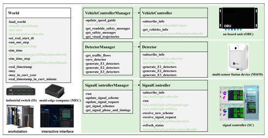
Figure 8.
In-the-Loop Simulation Platform.
4. Case Study
Given that the theoretical models and deployment architecture described in Section 2 and Section 3 have been successfully implemented in a real-world project on Chengaodadao, Conghua District, Guangzhou, this study selects real-world data from that arterial as the case study. The in-the-loop simulation platform is used to validate the applicability and effectiveness of the system under real operational conditions. The case study corridor contains 17 intersections and is divided into four subzones, as shown in Figure 9. Among them, Subzone 4 uses Hisense signal controllers, while the remaining subzones use SCATS signal controllers.
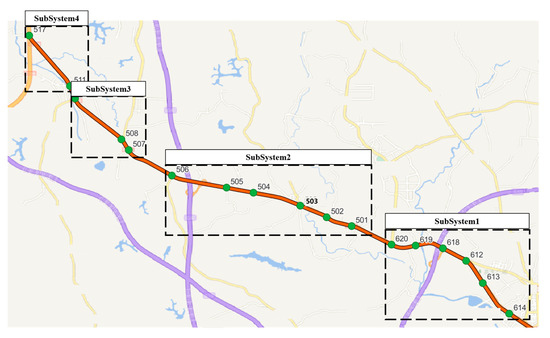
Figure 9.
Location of the Case Study Corridor.
Each approach of the 17 intersections in the corridor is equipped with Multi-Sensor Fusion Devices (MSFDs) capable of collecting 5 min traffic volume and queue length data for each entry lane. This study uses real data from 23 November 2024, from 00:00 to 23:59, for the analysis. The total 5 min traffic volume and maximum queue length at each intersection are shown in Figure 10. As the primary east–west commuter route in Conghua District, this corridor displays clear peak-hour patterns with distinct morning (7:30–9:00) and evening (17:30–19:00) peaks. The traffic volume data reveal several important characteristics. During the morning peak period, volumes surge sharply to reach 3000 vehicles per 5 min interval, with sustained high volumes exceeding 2500 vehicles throughout the peak. The evening peak shows slightly lower maximum volumes of 2000 vehicles per 5 min interval. The section between Intersections 612 and 619 experiences particularly heavy traffic flows, approximately 1.5 times the corridor average, due to its confluence with another major arterial road. Off-peak hours (10:00–16:00) show significantly lower volumes, typically below 500 vehicles per 5 min interval. Queue length measurements demonstrate that maximum queues reach up to 200 m during peak periods. Certain intersections consistently experience longer queues, particularly Intersections 502, 503, 511, and 517. The queue length data show strong correlation with the volume patterns, with the longest queues occurring during the highest volume periods. However, some intersections maintain elevated queue lengths even during moderate traffic conditions, suggesting potential capacity constraints or suboptimal signal timing at these locations.
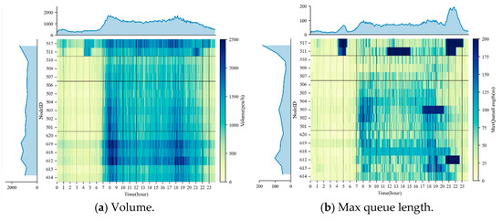
Figure 10.
Existing Traffic Volume and Maximum Queue Length at Each Intersection.
The data clearly illustrates the corridor’s critical role in commuter traffic, with the morning peak showing more intense congestion than the evening peak. The spatial analysis reveals specific bottleneck locations where targeted improvements could yield significant benefits. The temporal patterns provide valuable insights for developing time-dependent control strategies that could better accommodate the observed demand fluctuations.
The phase sequences for all 17 intersections in the corridor are listed in Table 3. The approach directions are denoted using eight compass directions: N, NW, W, SW, S, SE, E, and NE. The turning movements are represented as follows: “l” for left turn, “L” for partial left turn, “s” for through movement, and “r” for right turn. If a stage is reserved only for pedestrian movement, its phase label is marked as “ped”. The existing signal control mode is fixed-time control at isolated intersections, with the day divided into seven time periods, as follows: Period 2 (22:00–6:00), Period 3 (6:00–7:30), Period 4 (7:30–9:00), Period 5 (9:00–17:00), Period 6 (17:00–19:00), Period 7 (19:00–20:30), Period 1 (20:30–22:00). The current time period segmentation is reasonable and aligns well with the duration of the morning and evening peaks. The signal timing schemes for each time period are detailed in Appendix D, where each cell contains three numbers representing the green time, yellow time, and all-red time for each stage.
Table 3.
Mapping Between Stages and Permitted Phases at Each Intersection.
4.1. Error Analysis of the Delay Estimation Model
To verify the accuracy of the QEDM delay estimation model proposed in Section 2.1, the Webster model [6] and the QDM model [17,18] are selected as comparison baselines. To eliminate mutual interference between different movement directions within the intersection, a virtual simulation scenario with a single-lane, single-phase setup is created in SUMO for the experiments described in Section 4.1. The vehicle arrival rate is set to 0.1 pcu/s, and the signal cycle length is fixed at 100 s. The effective green time is varied from 95 s to 10 s in steps of 5 s to simulate various demand–supply conditions. The average vehicle delay reported by the E2 detector in the simulation is taken as the ground truth, and the error between each model’s computed value and true value is compared.
SUMO simulation parameters are as follows. The default Krauss car-following model is used. The headway is set to . The vehicle length and minimum gap are set to and . The desired speed of vehicles is set to . The theoretical saturation flow rate is calculated as . However, due to car-following behavior, the actual saturation flow rate observed in SUMO is approximately . To ensure consistency with the SUMO simulation environment, all delay models use . The delay estimation results of each model under different scenarios are shown in Table 4, where is effective green time. is initial queue length at the beginning of green and is the true value of delay from SUMO. is time required to clear the queue. is the number of cycles required for the last queued vehicle to clear the intersection. is the delay computed by the delay model. is the relative error of the delay model.
Table 4.
Comparison Between Delay Models and Ground Truth Under Different Supply–Demand Scenarios.
In Table 4, the signal cycle length remains fixed at 100 s, while the effective green time gradually decreases from 95 s to 10 s. As a result, the green time and green ratio (green time/cycle time) in each row are equivalent, reflecting different supply–demand scenarios. When the effective green time is greater than 25 s, the queue clearing time is shorter than the effective green time, corresponding to an undersaturated scenario, as illustrated in Figure 1a. When the effective green time drops to 25 s, the queue clearing time becomes 33.88 s, exceeding the available green time. The average delay increases sharply from 31.79 s to 52.13 s, while the number of cycles required for the last vehicle to leave the queue is still 1. This corresponds to an oversaturated scenario with residual queue dissipation, as shown in Figure 2a. As the effective green time continues to decrease, the number of cycles needed for the last queued vehicle to exit exceeds 1, indicating residual queue accumulation, i.e., an oversaturated scenario as in Figure 2b. In this condition, vehicle delay increases rapidly from 52.13 s to 421.63 s.
The delay estimation results from the various models are shown in Figure 11. Overall, all three delay models exhibit an exponential growth trend similar to the SUMO ground truth. However, the Webster model consistently overestimates delays across all scenarios. The QDM model, which does not account for multi-cycle evolution of residual queues, fails to reflect the delay increase under oversaturated conditions with accumulated queues (i.e., when green time is below 20 s). As a result, its estimated delay remains unchanged and significantly underestimates the true delay in this regime.
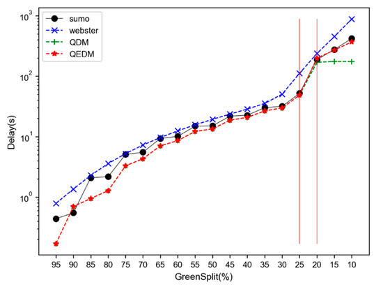
Figure 11.
Delay Estimation Results of Different Models.
The estimation errors of the delay models are shown in Figure 12. In Figure 12a, the Webster model consistently overestimates the delay compared to the ground truth, while both the QDM and QEDM models underestimate it slightly. Figure 12b shows that all three models exhibit relatively large estimation errors under low-demand scenarios where the green ratio exceeds 75%. This is because the delay estimation models assume a uniform arrival pattern using a linear approximation based on average arrival rates. However, in low-demand scenarios, arrival randomness is more pronounced, making it harder to estimate delays accurately. In contrast, under high-demand scenarios where the green ratio falls below 25%, the Webster and QDM models diverge sharply, as neither can accurately capture queue accumulation dynamics in oversaturated conditions. Meanwhile, the QEDM model shows a converging error trend as the green ratio decreases, which aligns with the findings of Mohajerpoor et al. [14] based on traffic wave theory. Table 5 summarizes the average estimation errors of all three models under undersaturated, oversaturated, and overall scenarios. The results show that the QEDM model consistently has the smallest absolute average error across all scenarios, improving upon the Webster and QDM models by 62% and 24%, respectively. Notably, because the QEDM model accurately describes queue evolution in oversaturated conditions, its average estimation error in those scenarios is only −3.5%, which represents an improvement of 95% over the Webster model and 87% over the QDM model.
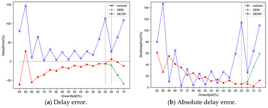
Figure 12.
Estimation Errors of Different Delay Models.
Table 5.
Average Estimation Error (%) of Each Delay Model.
4.2. Comparison of Control Mode
This section analyzes the control performance of three strategies using the case scenario shown in Figure 9 and Figure 10: fixed-time isolated control, coordinated control (with P1-2 and P2-2 updated every 30 min), and coordinated adaptive control (with P1-2 and P2-2 updated every 30 min, and P1-3 updated every 5 min). Figure 13 systematically evaluates traffic control performance across different time periods through six subplots, presenting metrics calculated at 30 min intervals. The figure provides a comprehensive comparison of three control strategies by examining their impacts on both coordinated-direction traffic flow and overall regional traffic conditions.
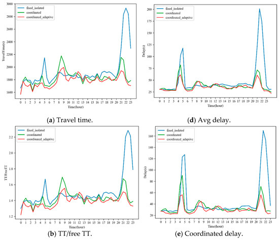
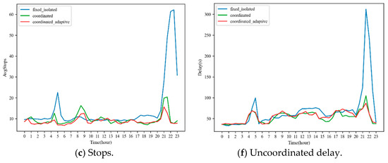
Figure 13.
Comparison of Control Strategy Performance.
The first three subplots (Figure 13a–c) concentrate on analyzing traffic performance in the coordinated direction. Figure 13a demonstrates that coordinated adaptive control consistently maintains the lowest average travel times across 17 consecutive intersections throughout most time periods, with particularly significant advantages during off-peak hours. In contrast, fixed-time control shows pronounced performance degradation at 5:00 and 22:30, coinciding with random traffic surges at Intersections 511 and 517 (as illustrated in Figure 10). These peaks clearly reveal fixed-time control’s inherent limitation in adapting to unpredictable traffic demand fluctuations. Figure 13b presents a normalized evaluation through the ratio of actual travel time to free-flow travel time, offering clearer insight into the performance gap relative to ideal conditions. Notably, coordinated adaptive control maintains this ratio below 1.4 for 85% of the time, substantially outperforming fixed-time control’s 60%. Figure 13c illustrates the average number of vehicle stops, including repeated acceleration–deceleration cycles caused by extended queuing. The temporal patterns in this subplot closely align with those in Figure 13a, establishing a direct correlation between stop frequency and overall travel time that validates the effectiveness of coordinated signal control in establishing green wave progression and reducing unnecessary stops.
The remaining three subplots (Figure 13d–f) assess the broader impacts on regional traffic conditions. Figure 13d shows average intersection delay, while Figure 13e and Figure 13f specifically examine delays in the coordinated and non-coordinated directions, respectively. Given that coordinated-direction delay equals the difference between travel time and free-flow travel time, Figure 13e naturally follows the same trend as Figure 13a. An important finding from Figure 13f is the differing impacts of the two observed demand fluctuation points. The 5:00 fluctuation shows significantly smaller delay increases in the non-coordinated direction compared to 22:30, suggesting that the earlier fluctuation primarily involved non-coordinated direction demand surges with relatively limited impact, whereas the later fluctuation likely involved more severe conditions such as intersection gridlock.
Collectively, these analyses demonstrate that coordinated adaptive control generally outperforms fixed-time control across most time periods. However, a notable limitation emerges during the 8:00–9:00 period, when both coordinated control and coordinated adaptive control (constrained by their 30 min coordination updates and approximately 10 min signal transition periods) exhibit slightly poorer performance than fixed-time control. This constraint arises because their real-time optimization relies on traffic demand data from the previous 30 min. To mitigate this issue, a potential solution would involve using historical morning peak (7:30–9:00) data to precompute coordination constraints at 7:00, allowing adaptive optimization during the actual peak period to operate within these pre-established parameters. This approach would effectively avoid disruptive signal transitions during the critical morning peak window while maintaining the benefits of adaptive control.
Table 6 presents a comprehensive performance evaluation of three distinct traffic control strategies through quantitative metrics collected over a full-day operational period. The comparative analysis yields several critical insights regarding the operational efficacy of fixed-time isolated control, coordinated control, and coordinated adaptive control methodologies. The performance enhancement patterns exhibit a well-defined hierarchical structure across various evaluation metrics. The most pronounced improvements manifest in the reduction of vehicular stops, where coordinated control demonstrates a substantial 32.4% decrease relative to fixed-time control. Coordinated adaptive control further augments this improvement by an additional 5.7 percentage points, achieving an overall 38.1% reduction. This remarkable decrease in stop frequency translates directly into enhanced fuel economy and diminished vehicular emissions, contributing to both operational efficiency and environmental sustainability. In terms of delay metrics, the analysis reveals consistent yet comparatively moderate enhancements. The coordinated control strategy reduces overall average delay by 22.8%, while the coordinated adaptive approach extends this improvement to 27.7%. Particularly noteworthy is the balanced performance between coordinated and non-coordinated directions, with coordinated adaptive control achieving delay reductions of 32.4% and 30.4%, respectively. This equilibrium underscores the adaptive methodology’s capability to optimize traffic flow network-wide without preferential treatment of coordinated directions. The travel time metrics, while exhibiting relatively smaller improvements, maintain statistical significance. Both absolute travel time and the travel time-to-free-flow time ratio show improvements of 5.3–5.4% under coordinated control, escalating to 7.9% with coordinated adaptive control. The identical enhancement percentages for these correlated metrics validate the methodological consistency across different performance measurement approaches.
Table 6.
All-Day Average Performance of Different Control Strategies.
A key finding demonstrates that coordinated adaptive control consistently surpasses basic coordinated control across all evaluated parameters, delivering additional improvements ranging from 2.6 percentage points (average delay) to 8.7 percentage points (coordinated direction delay). This substantiates the added value of integrating real-time adaptive optimization within the coordinated control framework. These empirical findings carry substantial implications for contemporary traffic management practices. The significant reductions in vehicular stops and network delays suggest that implementing coordinated adaptive control could yield measurable improvements in both traffic operational efficiency and environmental impact mitigation. The balanced performance across all network directions indicates that such implementations would benefit the entire transportation ecosystem, rather than privileging specific coordinated routes.
4.3. Comparison of Optimization Algorithms
The coordinated adaptive optimization framework proposed in Section 2.4 is compatible with various coordination optimization algorithms and isolated intersection optimization algorithms. In this section, nine combinations of optimization algorithms are selected and applied within the framework to evaluate how different algorithm choices affect control performance. The combinations are listed in Table 7. In particular, the “Webster-based” method used in Step Arterial-1 refers to the Webster timing method, which is not inherently an optimization algorithm and cannot incorporate coordination constraints. Therefore, in Step Intersection-1, the Webster delay formula is used to replace the delay estimation component in Model P1-3, thereby constructing a coordination-constrained version of adaptive optimization based on Webster.
Table 7.
Optimization Algorithm Combinations.
Figure 14 presents a comparative analysis of the all-day performance of nine different optimization algorithm combinations within the coordinated adaptive control framework. Figure 14a illustrates the distribution of average delays across all intersections and time periods for each combination; Figure 14b displays a comparison of the maximum queue clearance times; and Figure 14c summarizes the distribution of travel times for vehicles in the coordinated direction. Overall, the performance differences between the various coordination optimization algorithms (such as MaxBand, MultiBand, and AMBand) are relatively minor, indicating that the coordination-layer algorithms have a limited impact on the system’s overall performance. However, significant performance variations are observed at the isolated intersection optimization level: the QEDM-based method performs the best, followed by the Webster-based method, while the QDM-based method performs the worst. The root cause of this phenomenon lies in the different approaches these algorithms take in handling the dynamic relationship between queue length and signal cycle length. Specifically, the QDM-based method fails to establish a dynamic coupling relationship between cycle length and queue length. Its optimization process can only passively extend the cycle when queues are long and cannot proactively shorten the cycle during periods of low traffic demand to further reduce queues, resulting in insufficient system flexibility. The Webster-based method assumes that the number of vehicles arriving within a cycle is always positively correlated with the cycle length. This leads to a tendency to select longer cycles under undersaturated conditions, artificially “diluting” the average delay per vehicle to falsely meet optimization objectives. In practice, however, this often results in resource waste and response lag.
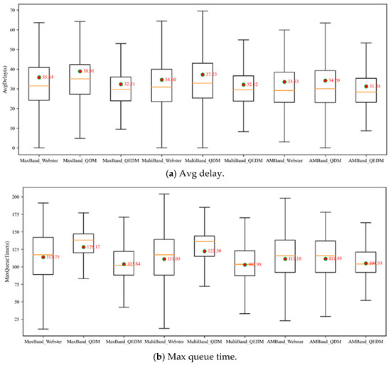
Figure 14.
Comparison of Optimization Algorithm Combinations.
To address these issues, this paper introduces constraints (12), (13), and (14) to correct the erroneous estimations of vehicle arrivals and queue dynamics in the optimization model. Additionally, constraint (6) is incorporated to accurately handle complex overlapping phase scenarios. Both theoretical analysis and the empirical results in Figure 14 demonstrate that the improved QEDM-based method can more accurately describe the evolution of traffic states, thereby achieving the best performance in isolated intersection optimization. It not only effectively curbs queue growth during high-demand periods but also proactively reduces cycle length during off-peak hours, enhancing system responsiveness and overall efficiency.
Figure 15 illustrates the time-varying trends of the common cycle length in each SubSystem under the coordinated adaptive optimization framework, where Maxband is used in Step Arterial-2 and combined with various isolated intersection optimization algorithms. In Figure 15a,b,d, the QDM-based method shows a tendency for the common cycle length to remain high once increased, forming a vicious cycle of “long queue → long cycle → long queue.” This results in a lack of adaptability in the cycle length relative to traffic demand. In Figure 15c, the QDM-based method shows slight variations in cycle length. This is because SubSystem 3 exhibits high randomness in traffic demand. Although the common cycle length is relatively long, short-term demand drops lead to a reduction in queue length. These results indicate that, despite advanced detection technologies providing queue length as a traffic indicator, improper use of queue length in control logic can yield worse results than using only traffic volume (e.g., as in the Webster-based method). Furthermore, in Figure 15, both the Webster-based and QEDM-based methods demonstrate real-time adaptability of the common cycle length to traffic demand. However, the QEDM-based method generally results in shorter cycle lengths during off-peak periods, because it incorporates constraint (14), which prevents the optimization from favoring longer cycles in moderately loaded periods in order to “dilute” per-vehicle delay. Figure 16, Figure 17 and Figure 18 further demonstrate the time-varying trends in maximum queue clearance time at each intersection under the QDM-based, Webster-based, and QEDM-based methods, respectively, reinforcing this conclusion.
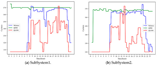
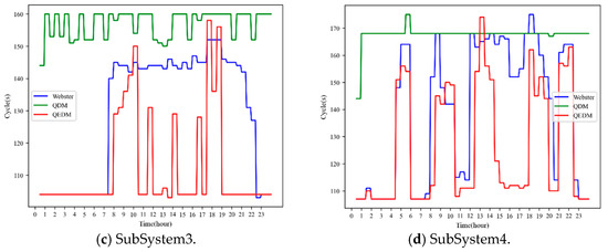
Figure 15.
Time-Varying Trends of Common Cycle Lengths in Each SubSystem.
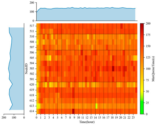
Figure 16.
Time-Varying Trends of Maximum Queue Clearance Time at Each Intersection (MaxBand + QDM-Based).
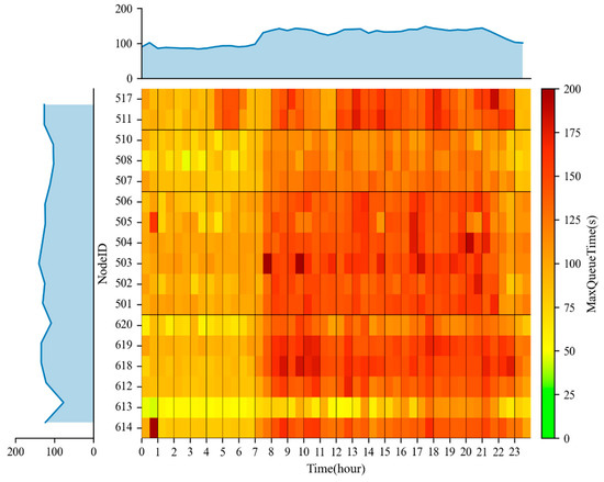
Figure 17.
Time-Varying Trends of Maximum Queue Clearance Time at Each Intersection (MaxBand + Webster-Based).
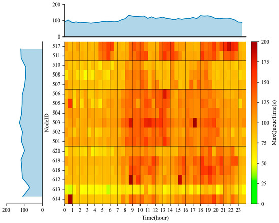
Figure 18.
Time-Varying Trends of Maximum Queue Clearance Time at Each Intersection (MaxBand + QEDM-Based).
4.4. Choice of Coordinated Constraints Update Interval
The update interval of coordination constraints is a critical parameter in the coordinated adaptive control method. If the update interval is too long, the coordination constraints will lag behind real-time traffic demand, which restricts the effectiveness of adaptive optimization. If the update interval is too short, the frequent changes in common cycle length and phase offsets will increase the signal transition time, leading to unstable signal control performance. The optimal update interval depends on multiple factors such as signal controller transition behavior, number of intersections, and traffic demand, and cannot be determined solely through mathematical optimization. In this section, we evaluate control performance under different update intervals by varying the interval in 5 min steps, using 30 min as the baseline, and testing intervals that are two steps shorter and two steps longer. Taking 30 min as an example, the signal transition states of each SubSystem are shown in Figure 19. In the figure, the solid line represents the common cycle length required by the coordination constraints. The shaded area represents the minimum and maximum actual cycle lengths across all intersections in the SubSystem at a given time. If the boundary of the shaded area does not coincide with the solid line, it indicates that the SubSystem is in a signal transition state at that time.
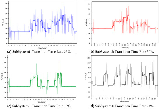
Figure 19.
Time-Varying Trends of Signal Transitions in Each Subsystem.
The proportion of transition time under different coordination update intervals is summarized in Table 8. As the update interval increases, the proportion of time spent in signal transitions gradually decreases across all SubSystems.
Table 8.
Proportion of Time in Signal Transition States.
Figure 20 shows the average delay, travel time in the coordinated direction, and average number of stops per vehicle during the morning peak period, under different update intervals. Control performance initially improves and then declines as the update interval increases, with 30 min identified as the optimal interval. The initial improvement is due to the reduction in transition time, which stabilizes control. The subsequent decline is caused by outdated coordination constraints, which hinder the adaptive optimizer’s ability to respond to real-time traffic demand.
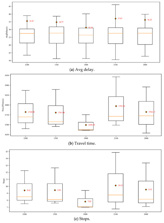
Figure 20.
Distribution of Morning Peak Control Performance Under Different Coordination Constraint Update Intervals.
5. Discussion
The results of this study demonstrate the efficacy of the proposed QEDM and the coordinated adaptive control framework in improving urban traffic performance. It is crucial to situate these findings within the broader context of the existing literature to highlight both the consistencies and the advancements this research offers.
5.1. Interpretation of Key Findings
The case study on the arterial road in Guangzhou revealed that the proposed coordinated adaptive control strategy achieved a 27.7% reduction in average delay and a 38.1% decrease in the number of stops compared to traditional fixed-time control. These significant improvements align with the general consensus in the field that adaptive and coordinated systems outperform static plans in dynamic urban environments [5,17]. More importantly, our method outperformed the 30 min update coordinated control, underscoring the value of high-frequency (5 min), constraint-based intersection-level optimization in fine-tuning traffic responsiveness. This finding addresses a critical gap noted by Wang et al. [25], whose framework limited optimization frequency, and extends the work of Hao et al. [30], Beak et al. [31], and Ma et al. [17] by effectively handling lagging coordinated phases and allowing for the shortening of green times, thus preserving the green band progression at the arterial level while fully leveraging the optimization potential of adaptive optimization at the intersection level.
5.2. Comparison with Existing Delay Estimation Models
The superior accuracy of QEDM, particularly in oversaturated conditions where it reduced the average estimation error to −3.5% compared to 78.25% for Webster and −27.75% for QDM, is a cornerstone of this study’s success. This result resonates with the work of Mohajerpoor et al. [14], who emphasized the importance of capturing queue evolution dynamics. While previous studies by Ma et al. [17] and Huang et al. [18] incorporated queue length into their models, our approach fundamentally differs by leveraging direct MSFD measurements to establish a clear, mathematical relationship between detected queue length and model parameters (e.g., Equations (12)–(14)). This moves beyond indirect inference from trajectory or LPR data [20,21], mitigating estimation errors and providing a more reliable foundation for optimization. The convergence of QEDM’s error as saturation increases validates its grounding in traffic flow theory.
5.3. The Role of the Coordination Framework and Deployment Architecture
The proposed cloud–edge–terminal architecture proved essential in operationalizing the theoretical models. This practical implementation bridges an often-overlooked gap between algorithm design and real-world deployment. Many theoretical studies on coordinated adaptive control [17,25,30] mention but do not fully address critical deployment challenges such as update intervals, signal transition times, and the integration of pedestrian phases. Our systematic incorporation of these factors into the modeling process (e.g., Equation (6) for overlapping phases) and the development of a standardized communication protocol (Table 2) ensure that the optimization outcomes are both practically feasible and executable. The hardware-in-the-loop simulation platform further enhances the credibility of the results by validating the entire control loop, not just the algorithm logic in isolation. This holistic approach to system design is a significant step towards the maturation of adaptive traffic control systems.
5.4. Trade-Offs and Optimal System Configuration
The analysis of coordination constraint update intervals revealed a critical trade-off. While shorter intervals (e.g., 20 min) allow coordination plans to be more responsive to real-time demand, they increase the proportion of time the system spends in disruptive signal transition states (up to 48%). Conversely, longer intervals (e.g., 40 min) stabilize operation but lead to outdated constraints that hinder adaptive optimization. The identification of a 30 min interval as the optimal balance for this specific corridor provides actionable guidance for traffic engineers. This empirical finding underscores that the performance of an adaptive system is not solely determined by its optimization algorithms but also by its operational parameters, a nuance that is frequently absent from purely simulation-based studies.
6. Conclusions, Limitations, and Further Research
6.1. Conclusions
This study presented a comprehensive solution for coordinated adaptive traffic signal control, encompassing a novel delay estimation model, an intersection-level optimization method, a multi-layer control framework, and a practical deployment architecture. The Queue Evolution and Delay Model (QEDM) was developed to explicitly link MSFD-measured queue data to delay calculations, dramatically improving estimation accuracy, especially in oversaturated conditions, which demonstrated a remarkable 95% improvement in delay estimation accuracy under oversaturated conditions compared to the Webster model, reducing the average estimation error from 78.25% to −3.5%. When compared to the QDM model, QEDM showed an 87% improvement in accuracy for oversaturated scenarios.
The proposed intersection-level optimization method proactively manages cycle lengths to dissipate queues and incorporates critical practical elements like pedestrian stages and overlapping phases. The coordinated adaptive control framework successfully balances arterial progression preservation with intersection-level adaptability, demonstrating compatibility with various optimization algorithms. Finally, the cloud–edge–terminal architecture and in-the-loop simulation platform effectively bridge the gap between theoretical research and practical engineering application. The implementation of our coordinated adaptive control framework yielded substantial operational benefits: travel time along coordinated directions was reduced by 7.9%, the average number of stops decreased by 38.1%, and overall delay saw a 27.7% reduction compared to conventional fixed-time control. These quantifiable improvements demonstrate the practical efficacy of integrating accurate queue length measurement through MSFD with an adaptive control strategy that maintains arterial progression while enabling intersection-level responsiveness.
6.2. Limitations
Despite the promising results, this study has several limitations. First, the performance of QEDM and the optimization models is contingent on the accuracy and reliability of the MSFD sensors. Sensor failure or data noise could degrade system performance. Second, the current model primarily focuses on vehicular traffic. While pedestrian phases are included as constraints, a more integrated optimization that simultaneously minimizes both vehicular and pedestrian delay could be explored. Finally, the impact of connected vehicles (CVs) providing richer data was not considered but represents a significant future direction.
6.3. Further Research
Future research will proceed in several directions:
- (1)
- Robustness and Resilience: Developing mechanisms to make the control system more robust to sensor failures or erroneous data, potentially through data fusion techniques and fault-tolerant algorithms.
- (2)
- Network-wide Application: Scaling the framework from arterial control to a network-wide level, investigating the interactions between multiple coordinated corridors and the resulting city-scale impacts.
- (3)
- Multi-Modal Integration: Expanding the optimization objectives to explicitly include public transit priority, pedestrian delay, and cyclist safety, fostering a more holistic urban mobility approach.
- (4)
- Connected and Autonomous Vehicles (CAVs): Exploring the transformative potential of CAV data (e.g., trajectory, intention) for predictive optimization and developing control strategies that leverage vehicle-to-infrastructure (V2I) communication to achieve unprecedented levels of efficiency and safety.
Author Contributions
Conceptualization, L.Y., R.H. and Y.W.; methodology, R.H. and Y.W.; software, R.H. and T.S.; validation, Y.W. and Z.W.; formal analysis, Y.W. and Z.W.; investigation, R.H., Y.W. and T.S.; resources, R.H. and T.S.; data curation, Y.W. and Z.W.; writing—original draft preparation, Z.W.; writing—review and editing, Y.W. and Z.W.; visualization, Y.W. and Z.W.; supervision, L.Y.; project administration, L.Y. All authors have read and agreed to the published version of the manuscript.
Funding
This research was funded by the National Natural Science Foundation of China, Grant No. 52402408.
Data Availability Statement
The original data presented in this study are openly available in Zenodo
at https://doi.org/10.5281/zenodo.17298996.
Conflicts of Interest
Author Yongjia Wang was employed by the company Zhao Bian (Shanghai) Technology Co., Ltd. The remaining authors declare that the research was conducted in the absence of any commercial or financial relationships that could be construed as a potential conflict of interest.
Correction Statement
This article has been republished with a minor correction to the Data Availability Statement. This change does not affect the scientific content of the article.
Appendix A
Appendix A.1. MSG_TrafficFlow
| Field Name | Type | Description |
| node_id | str | Node identifier in road network of the message |
| gen_time | int | Message generation time |
| stat_type | str | Statistical mode (e.g., time interval-based) |
| stats | [DF_TrafficFlowStat] | Collection of statistical indicators |
| time_records | str | Message block flow transfer records |
| msg_id | int | Message ID |
The collection of statistical indicators in Appendix A.1 is represented in the form of a TrafficFlowStat list, with field definitions provided in Appendix A.2.
Appendix A.2. DF_TrafficFlowStat
| Field Name | Type | Description |
| map_element | str | Lane ID |
| ptc_type | int | Type of Traffic Participant |
| veh_type | str | Vehicle Type |
| volume | int | Hourly Flow (0.01 pcu/h) |
| speed_point | int | Spot Speed (0.01 m/s) |
| speed_area | int | Section Average Speed (0.01 m/s) |
| density | int | Density (0.01 pcu/km/lane) |
| delay | int | Average Delay (0.1 sec/vehicle) |
| queue_length | int | Queue Length (0.1 m) |
| congestion | int | Congestion Index (0–255) |
| occupation | int | Space Occupancy Rate (0.01%) |
| time_headway | int | Headway (0.01 s) |
| space_headway | int | Spacing (0.01 m) |
| travel_time | int | Average Travel Time (0.1 s/vehicle) |
| green_utilization | int | Green Utilization Rate (0.01%) |
| saturation | int | Saturation (0.01%) |
| stops | int | Average Number of Stops per Vehicle (0.1 times) |
| queued_vehicles | int | Queue Vehicle Count (vehicles) |
| time_occupation | int | Time Occupancy Rate (0.01%) |
| ext | str | Extended Indicator Fields |
Appendix B
Appendix B.1. MSG_SignalScheme
| Field Name | Type | Description |
| scheme_id | int | Signal Control Plan ID |
| node_id | str | Associated Intersection |
| cycle | int | Cycle Length (s) |
| control_mode | str | Signal Control Mode |
| min_cycle | int | Minimum Cycle Length (s) |
| max_cycle | int | Maximum Cycle Length (s) |
| phases | [DF_Phasic] | Stage Information (Ordered by Appearance) |
| base_signal_scheme_id | int | Reference Signal Plan ID |
| offset | int | Offset (s) |
| time_records | str | Message Flow Transfer Records |
| msg_id | int | Unique Message ID |
| extra | str | Additional Description |
| source | str | Source of Signal Control Plan |
The collection of phase-based control indicators in Appendix B.1 is represented in the form of a DF_Phasic list, with field definitions provided in Appendix B.2.
Appendix B.2. DF_Phasic
| Field Name | Type | Description |
| id | int | Phase Stage ID |
| green | int | Green Time (s) |
| yellow | int | Yellow Time (s) |
| allred | int | All-Red Time (s) |
| scat_no | str | SCATS System Index |
| order | int | Stage Order in Plan |
| min_green | int | Minimum Green Time (s) |
| max_green | int | Maximum Green Time (s) |
| movements | [str] | Phase Extensions ID with Right-of-Way |
| late_starts | [str] | List of Phases with Delayed Green Start |
| early_ends | [str] | List of Phases with Early Green Termination |
| non_greens | [str] | Phases with Right-of-Way but No Green Display |
| green_flash | [str] | Green flash time adjustment for phases (s) |
| on_demand | bool | Whether it is an on-demand phase (for actuated/adaptive control) |
Appendix C
Appendix C.1. MSG_SignalRequest
| Field Name | Type | Description |
| control_mode | DE_SignalControlMode | Signal controller control mode |
| details | DF_SignalSchemeConstraint | Constraint details of the signal control plan |
| time_records | str | Message flow records |
| msg_id | int | Unique message ID |
| source | str | Source of signal control request |
Appendix C.2. DF_SignalSchemeConstraint
| Field Name | Type | Description |
| scheme_id | int | Signal control plan ID |
| node_id | str | Associated intersection ID |
| min_cycle | int | Minimum cycle length (s) |
| max_cycle | int | Maximum cycle length (s) |
| offset | int | Offset, used for coordination adjustment (s) |
| phasic_constraints | [DF_PhasicConstraint] | List of stage constraints, ordered sequentially |
Appendix C.3. DF_PhasicConstraint
| Field Name | Type | Description |
| id | int | Phase stage ID |
| expected_order | int | Expected order of the phase stage in the plan (starting from 0) |
| extra | str | Additional information |
| min_green | int | Minimum green time (s) |
| max_green | int | Maximum green time (s) |
Appendix D. Fixed-Time Control Stage Time
| Period | NodeId | Stage A | Stage B | Stage C | Stage D | Stage E | Cycle | Offset |
| 2 (22:00–6:00) | 517 | 15, 3, 0 | 21, 3, 0 | 15, 3, 0 | 15, 3, 0 | 19, 3, 0 | 100 | 0 |
| 511 | 15, 3, 0 | 15, 3, 0 | 15, 3, 0 | 0, 0, 28 | 15, 3, 0 | 100 | 0 | |
| 510 | 15, 3, 0 | 15, 3, 0 | 15, 3, 0 | 15, 3, 0 | 28, 0, 0 | 100 | 0 | |
| 508 | 15, 3, 0 | 33, 3, 0 | 15, 3, 0 | 28, 0, 0 | 100 | 0 | ||
| 507 | 15, 3, 0 | 15, 3, 0 | 15, 3, 0 | 15, 3, 0 | 0, 0, 28 | 100 | 0 | |
| 506 | 15, 3, 0 | 15, 3, 0 | 15, 3, 0 | 15, 3, 0 | 25, 3, 0 | 100 | 0 | |
| 505 | 0, 0, 28 | 15, 3, 0 | 15, 3, 0 | 15, 3, 0 | 15, 3, 0 | 100 | 0 | |
| 504 | 15, 3, 0 | 15, 3, 0 | 15, 3, 0 | 0, 0, 28 | 15, 3, 0 | 100 | 0 | |
| 503 | 15, 3, 0 | 15, 3, 0 | 15, 3, 0 | 0, 0, 28 | 15, 3, 0 | 100 | 0 | |
| 502 | 15, 3, 0 | 15, 3, 0 | 15, 3, 0 | 15, 3, 0 | 0, 0, 28 | 100 | 0 | |
| 501 | 15, 3, 0 | 15, 3, 0 | 15, 3, 0 | 15, 3, 0 | 0, 0, 28 | 100 | 0 | |
| 620 | 15, 3, 0 | 15, 3, 0 | 15, 3, 0 | 15, 3, 0 | 72 | 0 | ||
| 619 | 15, 3, 0 | 15, 3, 0 | 15, 3, 0 | 15, 3, 0 | 0, 0, 28 | 100 | 0 | |
| 618 | 15, 3, 0 | 15, 3, 0 | 15, 3, 0 | 15, 3, 0 | 72 | 0 | ||
| 612 | 15, 3, 0 | 15, 3, 0 | 15, 3, 0 | 18, 0, 0 | 25, 3, 0 | 100 | 0 | |
| 613 | 25, 3, 0 | 15, 3, 0 | 33, 3, 0 | 15, 3, 0 | 100 | 0 | ||
| 614 | 24, 3, 0 | 24, 3, 0 | 15, 3, 0 | 25, 3, 0 | 100 | 0 | ||
| 3 (6:00–7:30) | 517 | 27, 3, 0 | 21, 3, 0 | 15, 3, 0 | 15, 3, 0 | 19, 3, 0 | 112 | 0 |
| 511 | 21, 3, 0 | 15, 3, 0 | 15, 3, 0 | 0, 0, 28 | 21, 3, 0 | 112 | 0 | |
| 510 | 15, 3, 0 | 23, 3, 0 | 19, 3, 0 | 15, 3, 0 | 28, 0, 0 | 112 | 0 | |
| 508 | 15, 3, 0 | 41, 3, 0 | 19, 3, 0 | 28, 0, 0 | 112 | 0 | ||
| 507 | 15, 3, 0 | 21, 3, 0 | 15, 3, 0 | 21, 3, 0 | 0, 0, 28 | 112 | 0 | |
| 506 | 15, 3, 0 | 23, 3, 0 | 15, 3, 0 | 19, 3, 0 | 25, 3, 0 | 112 | 0 | |
| 505 | 0, 0, 28 | 15, 3, 0 | 15, 3, 0 | 27, 3, 0 | 15, 3, 0 | 112 | 0 | |
| 504 | 15, 3, 0 | 27, 3, 0 | 15, 3, 0 | 0, 0, 28 | 15, 3, 0 | 112 | 0 | |
| 503 | 15, 3, 0 | 27, 3, 0 | 15, 3, 0 | 0, 0, 28 | 15, 3, 0 | 112 | 0 | |
| 502 | 15, 3, 0 | 27, 3, 0 | 15, 3, 0 | 15, 3, 0 | 0, 0, 28 | 112 | 0 | |
| 501 | 15, 3, 0 | 27, 3, 0 | 15, 3, 0 | 15, 3, 0 | 0, 0, 28 | 112 | 0 | |
| 620 | 17, 3, 0 | 19, 3, 0 | 17, 3, 0 | 29, 3, 0 | 94 | 0 | ||
| 619 | 19, 3, 0 | 19, 3, 0 | 19, 3, 0 | 15, 3, 0 | 0, 0, 28 | 112 | 0 | |
| 618 | 21, 3, 0 | 21, 3, 0 | 15, 3, 0 | 15, 3, 0 | 84 | 0 | ||
| 612 | 23, 3, 0 | 19, 3, 0 | 15, 3, 0 | 18, 0, 0 | 25, 3, 0 | 112 | 0 | |
| 613 | 25, 3, 0 | 15, 3, 0 | 45, 3, 0 | 15, 3, 0 | 112 | 0 | ||
| 614 | 24, 3, 0 | 24, 3, 0 | 27, 3, 0 | 25, 3, 0 | 112 | 0 | ||
| 4 (7:30–9:00) | 517 | 51, 3, 0 | 25, 3, 0 | 15, 3, 0 | 23, 3, 0 | 19, 3, 0 | 148 | 0 |
| 511 | 31, 3, 0 | 15, 3, 0 | 19, 3, 0 | 0, 0, 28 | 31, 3, 0 | 136 | 0 | |
| 510 | 15, 3, 0 | 47, 3, 0 | 35, 3, 0 | 23, 3, 0 | 28, 0, 0 | 160 | 0 | |
| 508 | 23, 3, 0 | 61, 3, 0 | 39, 3, 0 | 28, 0, 0 | 160 | 0 | ||
| 507 | 23, 3, 0 | 37, 3, 0 | 23, 3, 0 | 37, 3, 0 | 0, 0, 28 | 160 | 0 | |
| 506 | 29, 3, 0 | 39, 3, 0 | 29, 3, 0 | 23, 3, 0 | 25, 3, 0 | 160 | 0 | |
| 505 | 0, 0, 28 | 19, 3, 0 | 23, 3, 0 | 55, 3, 0 | 23, 3, 0 | 160 | 0 | |
| 504 | 29, 3, 0 | 39, 3, 0 | 29, 3, 0 | 0, 0, 28 | 23, 3, 0 | 160 | 0 | |
| 503 | 31, 3, 0 | 51, 3, 0 | 15, 3, 0 | 0, 0, 28 | 23, 3, 0 | 160 | 0 | |
| 502 | 23, 3, 0 | 55, 3, 0 | 23, 3, 0 | 19, 3, 0 | 0, 0, 28 | 160 | 0 | |
| 501 | 19, 3, 0 | 59, 3, 0 | 19, 3, 0 | 23, 3, 0 | 0, 0, 28 | 160 | 0 | |
| 620 | 23, 3, 0 | 39, 3, 0 | 23, 3, 0 | 33, 3, 0 | 130 | 0 | ||
| 619 | 15, 3, 0 | 23, 3, 0 | 35, 3, 0 | 23, 3, 0 | 0, 0, 28 | 136 | 0 | |
| 618 | 43, 3, 0 | 43, 3, 0 | 19, 3, 0 | 15, 3, 0 | 132 | 0 | ||
| 612 | 55, 3, 0 | 27, 3, 0 | 23, 3, 0 | 18, 0, 0 | 25, 3, 0 | 160 | 0 | |
| 613 | 25, 3, 0 | 23, 3, 0 | 77, 3, 0 | 23, 3, 0 | 160 | 0 | ||
| 614 | 24, 3, 0 | 24, 3, 0 | 75, 3, 0 | 25, 3, 0 | 160 | 0 | ||
| 5 (9:00–17:00) | 517 | 43, 3, 0 | 25, 3, 0 | 15, 3, 0 | 19, 3, 0 | 19, 3, 0 | 136 | 0 |
| 511 | 25, 3, 0 | 15, 3, 0 | 19, 3, 0 | 0, 0, 28 | 25, 3, 0 | 124 | 0 | |
| 510 | 15, 3, 0 | 35, 3, 0 | 27, 3, 0 | 19, 3, 0 | 28, 0, 0 | 136 | 0 | |
| 508 | 19, 3, 0 | 49, 3, 0 | 31, 3, 0 | 28, 0, 0 | 136 | 0 | ||
| 507 | 19, 3, 0 | 29, 3, 0 | 19, 3, 0 | 29, 3, 0 | 0, 0, 28 | 136 | 0 | |
| 506 | 23, 3, 0 | 31, 3, 0 | 23, 3, 0 | 19, 3, 0 | 25, 3, 0 | 136 | 0 | |
| 505 | 0, 0, 28 | 19, 3, 0 | 19, 3, 0 | 39, 3, 0 | 19, 3, 0 | 136 | 0 | |
| 504 | 19, 3, 0 | 39, 3, 0 | 19, 3, 0 | 0, 0, 28 | 19, 3, 0 | 136 | 0 | |
| 503 | 23, 3, 0 | 39, 3, 0 | 15, 3, 0 | 0, 0, 28 | 19, 3, 0 | 136 | 0 | |
| 502 | 19, 3, 0 | 39, 3, 0 | 19, 3, 0 | 19, 3, 0 | 0, 0, 28 | 136 | 0 | |
| 501 | 19, 3, 0 | 39, 3, 0 | 19, 3, 0 | 19, 3, 0 | 0, 0, 28 | 136 | 0 | |
| 620 | 21, 3, 0 | 31, 3, 0 | 21, 3, 0 | 33, 3, 0 | 118 | 0 | ||
| 619 | 15, 3, 0 | 23, 3, 0 | 27, 3, 0 | 19, 3, 0 | 0, 0, 28 | 124 | 0 | |
| 618 | 31, 3, 0 | 31, 3, 0 | 19, 3, 0 | 15, 3, 0 | 108 | 0 | ||
| 612 | 39, 3, 0 | 23, 3, 0 | 19, 3, 0 | 18, 0, 0 | 25, 3, 0 | 136 | 0 | |
| 613 | 25, 3, 0 | 19, 3, 0 | 61, 3, 0 | 19, 3, 0 | 136 | 0 | ||
| 614 | 24, 3, 0 | 24, 3, 0 | 51, 3, 0 | 25, 3, 0 | 136 | 0 | ||
| 6 (17:00–20:30) | 517 | 51, 3, 0 | 25, 3, 0 | 15, 3, 0 | 23, 3, 0 | 19, 3, 0 | 148 | 0 |
| 511 | 35, 3, 0 | 15, 3, 0 | 23, 3, 0 | 0, 0, 28 | 35, 3, 0 | 148 | 0 | |
| 510 | 15, 3, 0 | 47, 3, 0 | 35, 3, 0 | 23, 3, 0 | 28, 0, 0 | 160 | 0 | |
| 508 | 23, 3, 0 | 61, 3, 0 | 39, 3, 0 | 28, 0, 0 | 160 | 0 | ||
| 507 | 23, 3, 0 | 37, 3, 0 | 23, 3, 0 | 37, 3, 0 | 0, 0, 28 | 160 | 0 | |
| 506 | 29, 3, 0 | 39, 3, 0 | 29, 3, 0 | 23, 3, 0 | 25, 3, 0 | 160 | 0 | |
| 505 | 0, 0, 28 | 19, 3, 0 | 23, 3, 0 | 55, 3, 0 | 23, 3, 0 | 160 | 0 | |
| 504 | 29, 3, 0 | 39, 3, 0 | 29, 3, 0 | 0, 0, 28 | 23, 3, 0 | 160 | 0 | |
| 503 | 31, 3, 0 | 51, 3, 0 | 15, 3, 0 | 0, 0, 28 | 23, 3, 0 | 160 | 0 | |
| 502 | 23, 3, 0 | 55, 3, 0 | 23, 3, 0 | 19, 3, 0 | 0, 0, 28 | 160 | 0 | |
| 501 | 19, 3, 0 | 59, 3, 0 | 19, 3, 0 | 23, 3, 0 | 0, 0, 28 | 160 | 0 | |
| 620 | 25, 3, 0 | 43, 3, 0 | 25, 3, 0 | 37, 3, 0 | 142 | 0 | ||
| 619 | 15, 3, 0 | 23, 3, 0 | 35, 3, 0 | 23, 3, 0 | 0, 0, 28 | 136 | 0 | |
| 618 | 43, 3, 0 | 43, 3, 0 | 19, 3, 0 | 15, 3, 0 | 132 | 0 | ||
| 612 | 55, 3, 0 | 27, 3, 0 | 23, 3, 0 | 18, 0, 0 | 25, 3, 0 | 160 | 0 | |
| 613 | 25, 3, 0 | 23, 3, 0 | 77, 3, 0 | 23, 3, 0 | 160 | 0 | ||
| 614 | 24, 3, 0 | 24, 3, 0 | 75, 3, 0 | 25, 3, 0 | 160 | 0 | ||
| 7 (8:30–22:00) | 517 | 43, 3, 0 | 25, 3, 0 | 15, 3, 0 | 19, 3, 0 | 19, 3, 0 | 136 | 0 |
| 511 | 25, 3, 0 | 15, 3, 0 | 19, 3, 0 | 0, 0, 28 | 25, 3, 0 | 124 | 0 | |
| 510 | 15, 3, 0 | 35, 3, 0 | 27, 3, 0 | 19, 3, 0 | 28, 0, 0 | 136 | 0 | |
| 508 | 19, 3, 0 | 45, 3, 0 | 23, 3, 0 | 28, 0, 0 | 124 | 0 | ||
| 507 | 19, 3, 0 | 29, 3, 0 | 19, 3, 0 | 29, 3, 0 | 0, 0, 28 | 136 | 0 | |
| 506 | 23, 3, 0 | 31, 3, 0 | 23, 3, 0 | 19, 3, 0 | 25, 3, 0 | 136 | 0 | |
| 505 | 0, 0, 28 | 19, 3, 0 | 19, 3, 0 | 39, 3, 0 | 19, 3, 0 | 136 | 0 | |
| 504 | 19, 3, 0 | 39, 3, 0 | 19, 3, 0 | 0, 0, 28 | 19, 3, 0 | 136 | 0 | |
| 503 | 23, 3, 0 | 39, 3, 0 | 15, 3, 0 | 0, 0, 28 | 19, 3, 0 | 136 | 0 | |
| 502 | 19, 3, 0 | 39, 3, 0 | 19, 3, 0 | 19, 3, 0 | 0, 0, 28 | 136 | 0 | |
| 501 | 19, 3, 0 | 39, 3, 0 | 19, 3, 0 | 19, 3, 0 | 0, 0, 28 | 136 | 0 | |
| 620 | 21, 3, 0 | 27, 3, 0 | 21, 3, 0 | 29, 3, 0 | 110 | 0 | ||
| 619 | 15, 3, 0 | 23, 3, 0 | 27, 3, 0 | 19, 3, 0 | 0, 0, 28 | 124 | 0 | |
| 618 | 31, 3, 0 | 31, 3, 0 | 19, 3, 0 | 15, 3, 0 | 108 | 0 | ||
| 612 | 39, 3, 0 | 23, 3, 0 | 19, 3, 0 | 18, 0, 0 | 25, 3, 0 | 136 | 0 | |
| 613 | 25, 3, 0 | 19, 3, 0 | 61, 3, 0 | 19, 3, 0 | 136 | 0 | ||
| 614 | 24, 3, 0 | 24, 3, 0 | 51, 3, 0 | 25, 3, 0 | 136 | 0 | ||
| 1 (22:00–6:00) | 517 | 35, 3, 0 | 21, 3, 0 | 15, 3, 0 | 19, 3, 0 | 19, 3, 0 | 124 | 0 |
| 511 | 21, 3, 0 | 15, 3, 0 | 15, 3, 0 | 0, 0, 28 | 21, 3, 0 | 112 | 0 | |
| 510 | 15, 3, 0 | 27, 3, 0 | 23, 3, 0 | 19, 3, 0 | 28, 0, 0 | 124 | 0 | |
| 508 | 15, 3, 0 | 37, 3, 0 | 23, 3, 0 | 28, 0, 0 | 112 | 0 | ||
| 507 | 19, 3, 0 | 23, 3, 0 | 19, 3, 0 | 23, 3, 0 | 0, 0, 28 | 124 | 0 | |
| 506 | 15, 3, 0 | 23, 3, 0 | 15, 3, 0 | 19, 3, 0 | 25, 3, 0 | 112 | 0 | |
| 505 | 0, 0, 28 | 15, 3, 0 | 19, 3, 0 | 31, 3, 0 | 19, 3, 0 | 124 | 0 | |
| 504 | 19, 3, 0 | 27, 3, 0 | 19, 3, 0 | 0, 0, 28 | 19, 3, 0 | 124 | 0 | |
| 503 | 15, 3, 0 | 27, 3, 0 | 15, 3, 0 | 0, 0, 28 | 15, 3, 0 | 112 | 0 | |
| 502 | 19, 3, 0 | 27, 3, 0 | 19, 3, 0 | 19, 3, 0 | 0, 0, 28 | 124 | 0 | |
| 501 | 19, 3, 0 | 27, 3, 0 | 19, 3, 0 | 19, 3, 0 | 0, 0, 28 | 124 | 0 | |
| 620 | 17, 3, 0 | 19, 3, 0 | 17, 3, 0 | 19, 3, 0 | 84 | 0 | ||
| 619 | 23, 3, 0 | 19, 3, 0 | 23, 3, 0 | 19, 3, 0 | 0, 0, 28 | 124 | 0 | |
| 618 | 27, 3, 0 | 27, 3, 0 | 15, 3, 0 | 15, 3, 0 | 96 | 0 | ||
| 612 | 31, 3, 0 | 19, 3, 0 | 19, 3, 0 | 18, 0, 0 | 25, 3, 0 | 124 | 0 | |
| 613 | 25, 3, 0 | 19, 3, 0 | 49, 3, 0 | 19, 3, 0 | 124 | 0 | ||
| 614 | 24, 3, 0 | 24, 3, 0 | 39, 3, 0 | 25, 3, 0 | 124 | 0 |
References
- INRIX. INRIX 2024 Global Traffic Scorecard; Retrieved from INRIX Blog: Urban Congestion in 2024 & Beyond; INRIX: Kirkland, DC, USA, 2025. [Google Scholar]
- International Energy Agency. Global Energy Review 2025; IEA: Paris, France, 2025; Available online: https://www.iea.org/reports/global-energy-review-2025 (accessed on 20 August 2025).
- Wang, Y.; Yang, X. Non-Conventional Lane Design and Control Coordination Optimization at Urban Road Intersections: Review and Prospects. Appl. Sci. 2025, 15, 6720. [Google Scholar] [CrossRef]
- Wang, Y.; Yang, X. The Key Technologies of New Generation Urban Traffic Control System Review and Prospect: Case by China. Appl. Sci. 2025, 15, 7195. [Google Scholar] [CrossRef]
- Urbanik, T. Signal Timing Manual, 2nd ed.; NCHRP National Cooperative Highway Research Program Report; Transportation Research Board of the National Academies: Washington, DC, USA, 2015; ISBN 978-0-309-30888-5. [Google Scholar]
- Webster, F.V. Traffic Signal Settings; Road Research Lab Tech Papers; The National Academies of Sciences, Engineering, and Medicine: Washington, DC, USA, 1958. [Google Scholar]
- Tang, K.; Nakamura, H.; Boltze, M.; Tian, Z. Global Practices on Road Traffic Signal Control: Fixed-Time Control at Isolated Intersections; WCTRS Book Series; Elsevier: Amsterdam, The Netherlands, 2019; ISBN 978-0-12-815302-4. [Google Scholar]
- Jiang, X.; Qiu, Y.; Ruan, S. An Approach to Optimize the Settings of Actuated Signals. J. Mod. Transport. 2011, 19, 68–74. [Google Scholar] [CrossRef]
- Zheng, X.; Recker, W.; Chu, L. Optimization of Control Parameters for Adaptive Traffic-Actuated Signal Control. J. Intell. Transp. Syst. 2010, 14, 95–108. [Google Scholar] [CrossRef]
- Zhang, X.; Fan, X.; Yu, S.; Shan, A.; Fan, S.; Xiao, Y.; Dang, F. Intersection Signal Timing Optimization: A Multi-Objective Evolutionary Algorithm. Sustainability 2022, 14, 1506. [Google Scholar] [CrossRef]
- Hajbabaie, A.; Benekohal, R.F. (Ray) Traffic Signal Timing Optimization: Choosing the Objective Function. Transp. Res. Rec. J. Transp. Res. Board 2013, 2355, 10–19. [Google Scholar] [CrossRef]
- Jamal, A.; Tauhidur Rahman, M.; Al-Ahmadi, H.M.; Ullah, I.; Zahid, M. Intelligent Intersection Control for Delay Optimization: Using Meta-Heuristic Search Algorithms. Sustainability 2020, 12, 1896. [Google Scholar] [CrossRef]
- Wang, Z.; Chen, S.; Yang, H.; Wu, B.; Wang, Y. Comparison of Delay Estimation Models for Signalised Intersections Using Field Observations in Shanghai. IET Intell. Transp. Syst. 2016, 10, 165–174. [Google Scholar] [CrossRef]
- Mohajerpoor, R.; Saberi, M.; Ramezani, M. Analytical Derivation of the Optimal Traffic Signal Timing: Minimizing Delay Variability and Spillback Probability for Undersaturated Intersections. Transp. Res. Part B Methodol. 2019, 119, 45–68. [Google Scholar] [CrossRef]
- Lee, S.; Wong, S.C.; Varaiya, P. Group-Based Hierarchical Adaptive Traffic-Signal Control Part I: Formulation. Transp. Res. Part B Methodol. 2017, 105, 1–18. [Google Scholar] [CrossRef]
- Lee, S.; Wong, S.C.; Varaiya, P. Group-Based Hierarchical Adaptive Traffic-Signal Control Part II: Implementation. Transp. Res. Part B Methodol. 2017, 104, 376–397. [Google Scholar] [CrossRef]
- Ma, W.; An, K.; Lo, H.K. Multi-Stage Stochastic Program to Optimize Signal Timings under Coordinated Adaptive Control. Transp. Res. Part C Emerg. Technol. 2016, 72, 342–359. [Google Scholar] [CrossRef]
- Huang, W.; Cheng, H.; Huang, G.; Li, L. Integrated Optimization of Lane Allocation and Adaptive Signal Control at Isolated Intersection under Stochastic Demand. Transp. Res. Part C Emerg. Technol. 2024, 169, 104862. [Google Scholar] [CrossRef]
- Yao, Z.; Jiang, Y.; Zhao, B.; Luo, X.; Peng, B. A Dynamic Optimization Method for Adaptive Signal Control in a Connected Vehicle Environment. J. Intell. Transp. Syst. 2020, 24, 184–200. [Google Scholar] [CrossRef]
- Luo, L.; Wu, H.; Liu, J.; Tang, K.; Tan, C. A Probabilistic Approach for Queue Length Estimation Using License Plate Recognition Data: Considering Overtaking in Multi-Lane Scenarios. Transp. Res. Part C Emerg. Technol. 2025, 173, 105029. [Google Scholar] [CrossRef]
- Wang, Y.; Liu, Y.; Yang, X. A Novel Method for Traffic Parameter Extraction and Analysis Based on Vehicle Trajectory Data for Signal Control Optimization. Appl. Sci. 2025, 15, 7155. [Google Scholar] [CrossRef]
- Yu, S.; Wang, X.; Ci, Y.; Li, Y.; Zhou, M.; Dong, X.; Cai, M. MSPE-Fusion: A Multimodal 3D Object Detection Method with Multi-Sensor Perception Enhanced Fusion. Neurocomputing 2025, 645, 130486. [Google Scholar] [CrossRef]
- Alaba, S.Y.; Gurbuz, A.C.; Ball, J.E. Emerging Trends in Autonomous Vehicle Perception: Multimodal Fusion for 3D Object Detection. World Electr. Veh. J. 2024, 15, 20. [Google Scholar] [CrossRef]
- Onsu, M.A.; Simsek, M.; Fobert, M.; Kantarci, B. Intelligent Multi-Sensor Fusion and Anomaly Detection in Vehicles via Deep Learning. Internet Things 2025, 31, 101561. [Google Scholar] [CrossRef]
- Wang, Q.; Yuan, Y.; Yang, X.T.; Huang, Z. Adaptive and Multi-Path Progression Signal Control under Connected Vehicle Environment. Transp. Res. Part C Emerg. Technol. 2021, 124, 102965. [Google Scholar] [CrossRef]
- Chen, Y.-H.; Cheng, Y.; Chang, G.-L. Design of an Arterial Signal Progression Plan for Multi-Path Flows with Only Intersection Turning Counts. Transp. Res. Part C Emerg. Technol. 2021, 130, 103322. [Google Scholar] [CrossRef]
- Little, J.D.C.; Kelson, M.D.; Gartner, N.H. A Versatile Program for Setting Signals on Arteries and Triangular Networks. Available online: https://dspace.mit.edu/bitstream/handle/1721.1/1979/SWP-1185-08951478.pdf?sequence=1 (accessed on 20 August 2025).
- Gartner, N.H.; Assmann, S.F.; Lasaga, F.; Hous, D.L. MULTIBAND-A Variable-Bandwidth Arterial Progression Scheme. Transp. Res. Rec. 1990, 212–222, ISBN 0309050626. [Google Scholar]
- Zhang, C.; Xie, Y.; Gartner, N.H.; Stamatiadis, C.; Arsava, T. AM-Band: An Asymmetrical Multi-Band Model for Arterial Traffic Signal Coordination. Transp. Res. Part C Emerg. Technol. 2015, 58, 515–531. [Google Scholar] [CrossRef]
- Hao, B.; Lv, B.; Chen, Q.; Li, X. A Two-Stage Real-Time Optimization Model of Arterial Signal Coordination Based on Reverse Causal-Effect Modeling Approach. Sustainability 2023, 15, 14035. [Google Scholar] [CrossRef]
- Beak, B.; Head, K.L.; Feng, Y. Adaptive Coordination Based on Connected Vehicle Technology. Transp. Res. Rec. J. Transp. Res. Board 2017, 2619, 1–12. [Google Scholar] [CrossRef]
- Lopez, P.A.; Wiessner, E.; Behrisch, M.; Bieker-Walz, L.; Erdmann, J.; Flotterod, Y.-P.; Hilbrich, R.; Lucken, L.; Rummel, J.; Wagner, P. Microscopic Traffic Simulation Using SUMO. In Proceedings of the 2018 21st International Conference on Intelligent Transportation Systems (ITSC), Maui, HI, USA, 4–7 November 2018; pp. 2575–2582. [Google Scholar]
- Shanghai Intelligent New Energy Vehicle Big Data Competition. Available online: https://www.heywhale.com/home/competition/66a01e47981b6a298d91b9d4/content/3 (accessed on 9 June 2025).


Disclaimer/Publisher’s Note: The statements, opinions and data contained in all publications are solely those of the individual author(s) and contributor(s) and not of MDPI and/or the editor(s). MDPI and/or the editor(s) disclaim responsibility for any injury to people or property resulting from any ideas, methods, instructions or products referred to in the content. |
© 2025 by the authors. Licensee MDPI, Basel, Switzerland. This article is an open access article distributed under the terms and conditions of the Creative Commons Attribution (CC BY) license (https://creativecommons.org/licenses/by/4.0/).