Feature Extractor for Damage Localization on Composite-Overwrapped Pressure Vessel Based on Signal Similarity Using Ultrasonic Guided Waves

Abstract

Hydrogen is one of the future green energy sources that could resolve issues related to fossil fuels. The widespread use of hydrogen can be enabled by composite-overwrapped pressure vessels for storage. It offers advantages due to its low weight and improved mechanical performance. However, the safe storage of hydrogen requires continuous monitoring. Combining ultrasonic guided waves with interpretable machine learning provides a powerful tool for structural health monitoring. In this study, we developed a feature extraction approach based on a similarity method that enables interpretability in the proposed machine learning model for damage detection and localization in pressure vessels. Furthermore, a systematic optimization was performed to explore and tune the model’s parameters. This resulting model provides accurate damage localization and is capable of detecting and localizing damage on hydrogen pressure vessels with an average localization error of 2 cm and a classification accuracy of 96.5% when using quantized classification. In contrast, binarized classification yields a higher accuracy of 99.5%, but with a larger localization error of 6 cm.

1. Introduction

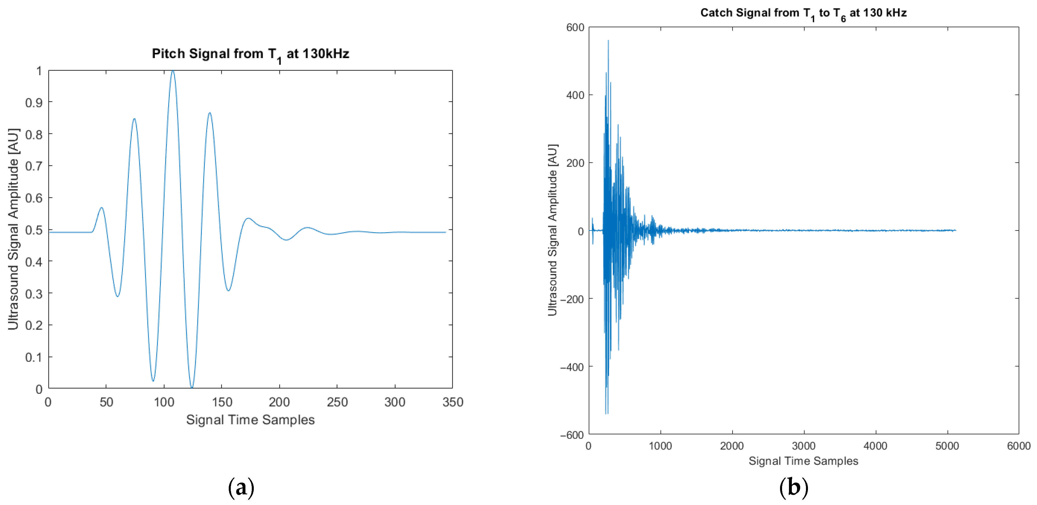
To ensure the safe storage of hydrogen in composite-overwrapped pressure vessels (COPVs) [1], the development of structural health monitoring (SHM) technologies is essential. These technologies help ensure the vessel remains in proper conditions by detecting damage that may occur during operation. Ultrasonic guided waves (UGWs) are a non-destructive testing method employed to inspect COPVs using the pitch–catch procedure [2]. It offers the advantage of covering a large area by exploiting the reflection and absorption properties of the ultrasonic waves (Figure 1) [3]. In this procedure, ultrasonic sensors are piezoelectric transducers that serve as transmitters when emitting UGW signals and as receivers when capturing the propagated waves (Figure 2). However, signal interpretation poses a challenge in ensuring accurate detection with minimal false alarms.

Several approaches based on machine learning (ML) have been developed to evaluate the acquired signals and detect damage. A strategy that elaborates a feature extractor based on signal difference was previously proposed. However, this signal difference approach is restrictive and can be generalized to overcome potential overfitting [4]. Deep learning-based approaches tend to overfit and are challenging to interpret, which is crucial when inspecting critical infrastructures [5]. Furthermore, software implementation errors are more likely to remain undetected and can be difficult to identify, as deep learning implementations are based on complex software. This is also the reason why security vulnerabilities present in the frameworks used for development, such as system compromise, the evasion of detection, and denial-of-service risks, are implicitly inherited by the developers [6]. On the other hand, training deep learning models for small datasets, i.e., those with a limited number of examples, allows for building only simple models that lack validation under operational conditions [7].

Another approach to investigating UGW and detecting damage is the Reconstruction Algorithm for Probabilistic Inspection (RAPID), a robust probabilistic imaging approach [8]. RAPID estimates the probability of damage between a transducer and a receiver by calculating the Pearson correlation between the measured signal and a baseline signal recorded under damage-free conditions [9]. A lower correlation indicates a higher likelihood of damage. A tomogram is generated by aggregating spotlights with their intensities determined by the calculated damage probabilities. However, this approach has limited precision due to the restricted resolution of the tomogram in identifying damage locations. This limitation stems from the simplification of plotting the spotlight with a constant ellipsoidal diameter ratio [10].

In this work, we develop and investigate an interpretable ML algorithm based on signal similarity as a feature extractor [11]. Within this approach, UGW signals of a COPV in an undamaged state are compared to UGW signals in a damaged state. The comparison involves segmenting the signals into equal-sized intervals and then applying a similarity measure, such as cross-correlation, to each corresponding interval to extract features that describe the presence of damage. The extracted features are labeled with quantized distances of the damage positions to the corresponding pitch–catch sensor pairs. A cutoff is applied to distances belonging to sensor pairs that are less influenced by the present damage. Although this approach has been proposed in a previous study [12], many questions remain open regarding the selection of adequate operational and hyperparameters, such as the optimal operational frequency, signal segmentation interval, applied quantization, and cutoff value. Furthermore, when validating using Leave-One-Group-Out Cross-Validation (LOGO-CV) [13], the test set is created by leaving out one pair of sensors across all damage configurations, which does not represent a practical scenario in real-world applications [12].

2. Materials and Methods

In this section, we present the design of the experimental campaign used to acquire the UGW signals employed for developing the machine learning algorithm. We then discuss the developed algorithm and the steps taken to achieve these results.

2.1. Design of Experiments

In the first development step, ultrasonic signal data need to be acquired from COPVs with reversible damage, simulated by weights glued to the surface of the vessel. For our study, an experiment was designed by using a COPV (NPROXX) with a length of 1670 mm and a perimeter of 352 mm that can withstand pressures up to 700 bar (Figure 3a). It is equipped with a network of 15 piezoelectric transducers (PI Ceramics, DuraAct patches of type P 876K025) (Figure 3b) [14]. These piezoelectric sensors function as transmitters and receivers, as required for the pitch–catch procedure.

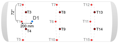
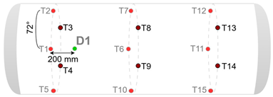
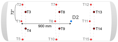
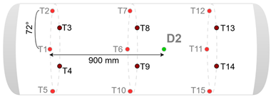
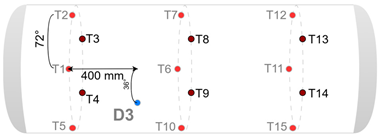
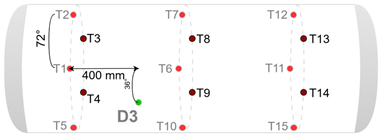
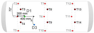
The 15 employed sensor transducers result in 210 pair combinations. For symmetry reasons and due to the transmission direction, only half of the combinations consisting of 105 pairs are finally considered ($15 Transducers\times {\displaystyle \frac{15 Transducers-1}{2}}=105$). This helps reduce the amount of acquired data, as sensor path $T_i{R}_j$ is covered by sensor path ${R_{i}T}_j$, where $i$, $j$ ∈ {1, 15} indicate the piezoelectric sensors. The sensor arrangement is based on previous work that investigated a carbon fiber-reinforced plastic plate [15]. Data acquisition is performed by connecting the sensor to a Vantage 64 LF acquisition system (Verasonic, Kirkland, WA, USA). The experiment begins with the measurement of baseline data at a constant temperature of 20 °C. The baseline data are necessary to detect any deviation from the undamaged state [16]. In the next step, reversible damage was introduced by gluing metal blocks of two different weights (330 g and 513 g) with a rectangular contact area of 24 cm² onto the COPV surface. This method is widely used for the non-destructive testing of COPVs as the attached weights mimic alterations in surface stiffness and acoustic impedance that would similarly result from real damage. Each weight was tested separately at three different positions, D₁, D₂, and D₃. Furthermore, two combinations of both weights were also tested on the COPV.

Table 1. Damage configurations of the eight conducted measurements with the weights used to add reversible damage. The green dots mark the 513 g weight, while the blue dots mark the 330 g weight. The lighter red dots represent the transducers located above the vessel, while the darker red dots represent the transducers on the opposite side of the vessel.

Damage ID	Damage Configuration
1
2
3
4
5
6
7
8

lists the eight measurements conducted using reversible damage, representing eight damage configurations.

A total of 840 signals ($8 experiments \times 105 pairs$) representing various cases of damage were measured, in addition to 105 baseline signals. For the experiment, we used a frequency of 130 kHz, which is suitable for detecting damage of the size introduced in this study. This can be verified based on wavelength $\lambda$ under the approximate ultrasound propagation speed, $c$, of 3042 m/s in the transverse direction of 90° in the investigated composite fiber material [17]. The minimal detectable damage size, $S_{min}$, is calculated using Formula (1) and yields a minimal detection size of approximately 6 mm at a frequency of 130 kHz [18]. The chosen frequency, as indicated by the dispersion curve for the vessel material, falls within a range where the A0 mode exhibits low group velocity and a dominant out-of-plane displacement. This makes it highly sensitive to local stiffness and mass changes, such as those simulated by the glued-on weights in this experiment, and similar to how it interacts with delaminations in composite materials [19,20].

$$S_{min}=\lambda /4={\displaystyle \raisebox{1ex}{$c$}\!\left/ \!\raisebox{-1ex}{$4f$}\right.}$$

(1)

2.2. Signal Evaluation Methods

This study aims to develop and optimize an interpretable ML algorithm able to detect and localize damage on a COPV. The approach is based on feature extraction, feature selection, and classification steps (FESC) [21]. This procedure delivers an interpretable result, overcoming the drawbacks of black-box models such as deep learning, which are not suitable for deployment in monitoring critical infrastructures.

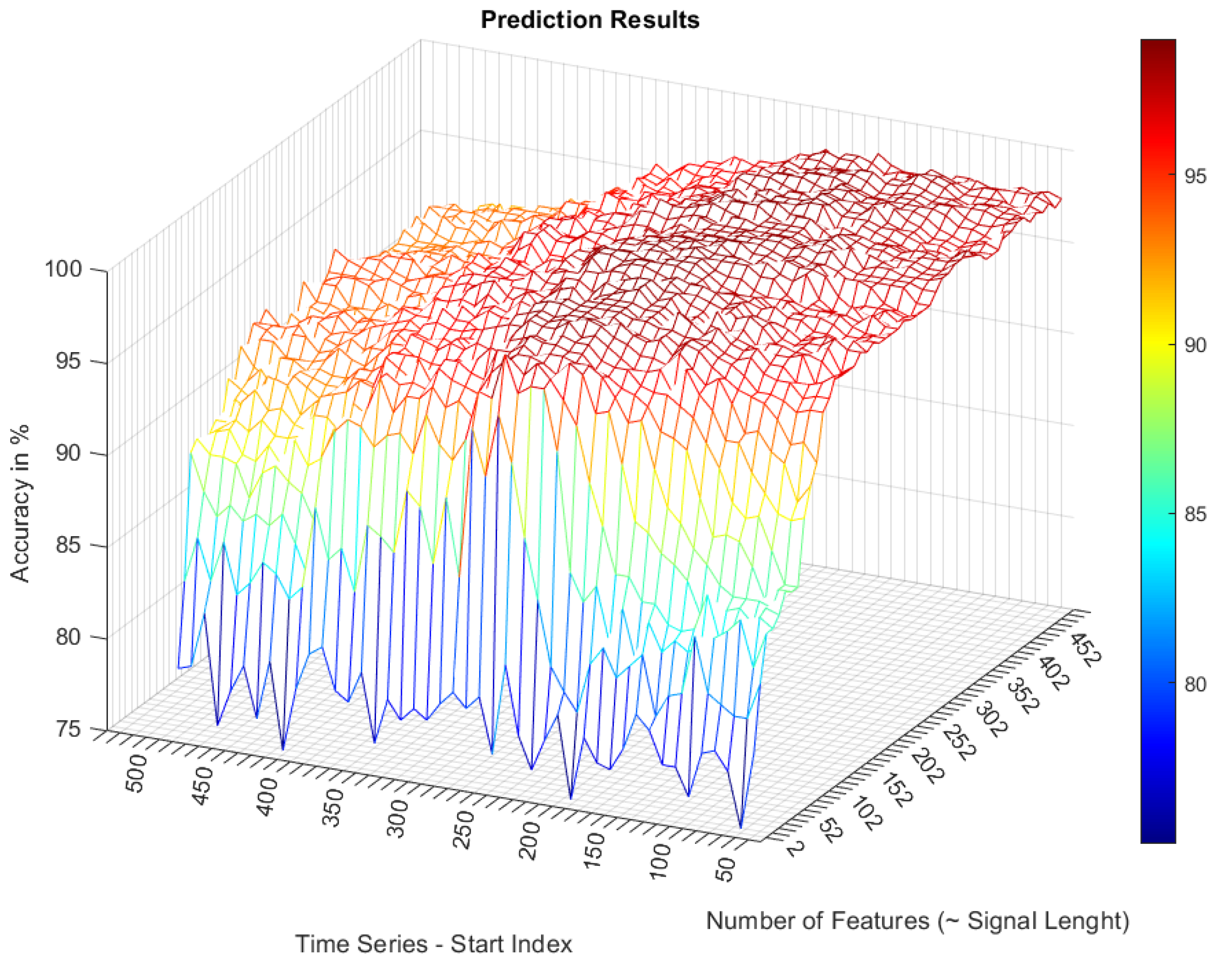
Before feature extraction, signal preprocessing is applied, which involves windowing to isolate the parts of the signal that contain information related to the damage (Figure 4). To determine the optimal windowing interval, windows with varying start and end data points were evaluated, and the configuration that achieved the highest accuracy was selected. The accuracy is calculated by comparing the predicted scores with the target variable. The length of the target variable then normalizes the number of predictions. The start values range from 10 to 500 in steps of 10 (i.e., 10, 20, …, 500), while the end points are obtained by adding values from interval 5 to 1000 (in steps of 10) to each start value. Following this, the feature extraction step, which is based on the signal similarity approach, is performed [12]. This approach involves splitting the signal time series into equal intervals, which are then compared to the corresponding intervals of a baseline time series using a similarity measure based on the normalized root mean square deviation (NRMSD) [22]. This method has been shown to provide the highest prediction accuracy and the lowest localization error [12]. In the segmentation step, the smallest segment length consisting of two data points was chosen to capture all signal changes. Further investigation into longer segment lengths will be conducted in future work. In the next step, each segment interval is compared with the corresponding interval from the baseline signal using the NRMSD similarity measure to calculate physics-informed features that enable interpretability. The approach assumes that lower similarity corresponds to a higher likelihood of damage. A value of 1 indicates the lowest similarity (i.e., the highest likelihood of damage), while a value of 0 indicates the highest similarity (i.e., no damage).

Figure 5 shows an example result of the NRMSD similarity measure, as defined in Formula (2), applied to the full signal length. Additionally, it illustrates the segmentation as divided into 100 segments, each corresponding to a distinct feature.

$${NRMSD}_i={\displaystyle \frac{\sqrt{\frac{\sum _{\mathrm{j}=(\mathrm{i}-1)\ast \mathrm{L}+1}^{\mathrm{i}\ast \mathrm{L}}{({\left(S_B\right)}_j-{\left(S_D\right)}_j)}^2}{L}}}{\mathrm{m}\mathrm{a}\mathrm{x}\left(S_D\right)-\mathrm{m}\mathrm{i}\mathrm{n}\left(S_D\right)}}$$

(2)

i: Segment index

j: Sample index within segment interval

L: The length of the segmented signal

S_B: Baseline signal

S_D: Damage-affected signal

Figure 5. Comparison between baseline in blue and signal affected by damage in red color for UGW propagating between transducer T₁ and receiver T₆. Segmentation interval of 100 that corresponds to 51 samples is shown by vertical discontinuous lines. Calculated similarity values between baseline and damage signals based on NRMSD are shown correspondingly for each segment in magenta color. Similarity measure of 1 indicates lower similarity and hence the presence of a damage.

Figure 5. Comparison between baseline in blue and signal affected by damage in red color for UGW propagating between transducer T₁ and receiver T₆. Segmentation interval of 100 that corresponds to 51 samples is shown by vertical discontinuous lines. Calculated similarity values between baseline and damage signals based on NRMSD are shown correspondingly for each segment in magenta color. Similarity measure of 1 indicates lower similarity and hence the presence of a damage.

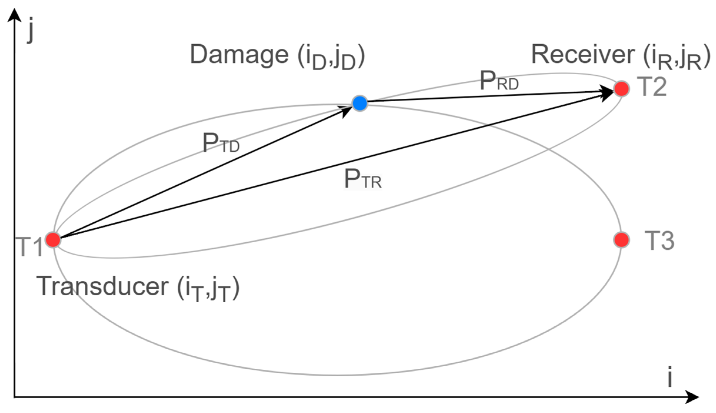
The next step involves standardizing the features because classification is later performed using Support Vector Machines (SVMs), which, like most classifiers, are sensitive to feature scaling. Finally, we apply an SVM for classification based on MATLAB’s standard implementation (version R2022b, The MathWorks, Inc., Natick, MA, USA), using the extracted features calculated according to Formula (2). This implementation employs a radial basis kernel, with the C parameter set to 1000, and an auto-selected kernel scale gamma determined using the subsampling heuristic procedure [23,24]. The classifier is trained on binary classes: class 1 refers to sensor transducer pairs that are significantly affected by damage, while class 0 represents unaffected pairs. In the first step, a diameter ratio is calculated based on the ellipsoids formed by ultrasonic wave propagation between transmitters and receivers that intersect at the damage location [25]. The diameter ratio is defined in Formula (3).

$$R_{Ø}={\displaystyle \frac{P_{TR}}{P_{TD}+P_{RD}}}={\displaystyle \frac{\sqrt{{(i_T-i_R)}^2+{(j_T-j_R)}^2}}{\sqrt{{(i_T-i_D)}^2+{(j_T-j_D)}^2}+\sqrt{{(i_R-i_D)}^2+{(j_R-j_D)}^2}}}$$

(3)

$R_{Ø}$: The diameter ratio of the ellipsoid starting at transducer T and arriving at receiver R over damage D.

$P_{TR}$: The direct path of the ultrasonic wave starting at transducer T and arriving at receiver R.

$P_{TD}$: Ultrasonic wave propagation starting at transducer T and arriving at damage D.

$P_{RD}$: Ultrasonic wave propagation reflected by damage D and arriving at receiver R.

($i_T,j_T$): Cartesian coordinates of the transducer position.

($i_R,j_R$): Cartesian coordinates of the receiver position.

($i_D,j_D$): Cartesian coordinates of the damage position.

A diameter ratio close to one indicates that the damage is along the direct path between the transducer and receiver pair. Conversely, a ratio near zero suggests the damage is far from the direct path and will have little or no impact on the signals of that transducer–receiver pair. Figure 6 illustrates the calculation of the diameter ratio using triangulation [25]. During this step, we apply a cutoff of 0.9 to the diameter ratio, as suggested in the RAPID implementation [8], creating an interest interval of [0.9, 1]. Only damage with a diameter ratio within this range is considered to affect the corresponding sensor pair. Then, a threshold within this interval is chosen to optimize model accuracy. The binarization process is shown in Formula (4).

Figure 6. Triangulation for calculating the diameter ratios of damage D between transducer–receiver pairs. The red dots represent the transducers, while the blue dots represent the damage location.

Figure 6. Triangulation for calculating the diameter ratios of damage D between transducer–receiver pairs. The red dots represent the transducers, while the blue dots represent the damage location.

$$R_B=\left\{\begin{array}{c}1, R_{Ø}\ge R_{th} \\ 0,R_{Ø}<R_{th} \end{array}\right.$$

(4)

$R_B$: The binarized diameter ratio used for classification.

$R_{Ø}$: The diameter ratio.

$R_{th}$: The diameter ratio threshold that lies within the interval of interest [0.9, 1].

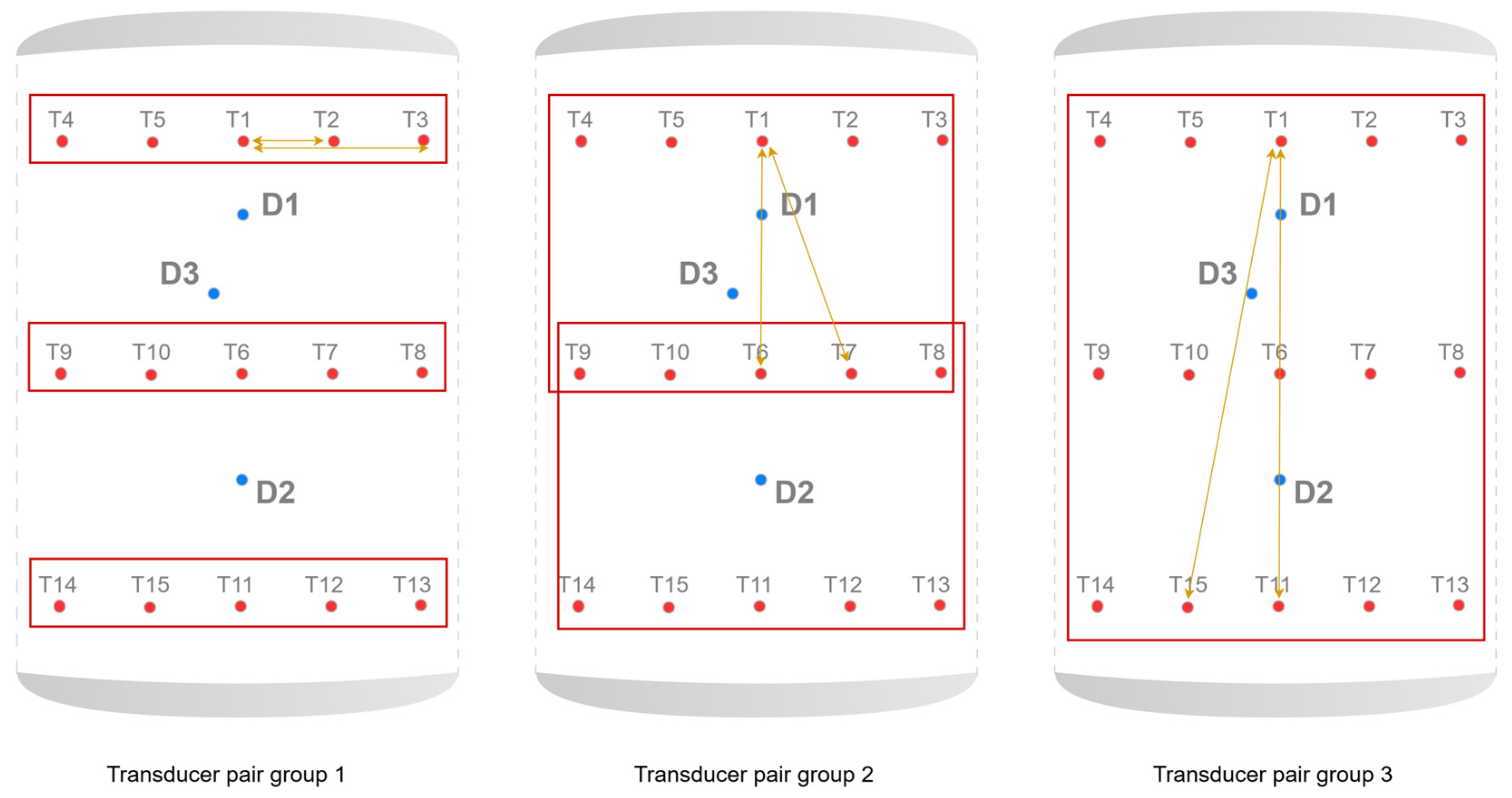
To enhance the method’s robustness, the sensor transducer pairs are divided into three groups [26]. The first group includes pairs located within the same sensor ring. The second group consists of pairs formed by transducers from neighboring rings. The third group consists of pairs where transmitters are located on the upper ring and receivers on the lower ring. In this study, only transducer pairs from the second group are used, as pairs from the first group were unaffected by the damage introduced and were consistently labeled as 0. Pairs from the third group are also excluded because damage is more effectively detected by the second group (Figure 7).

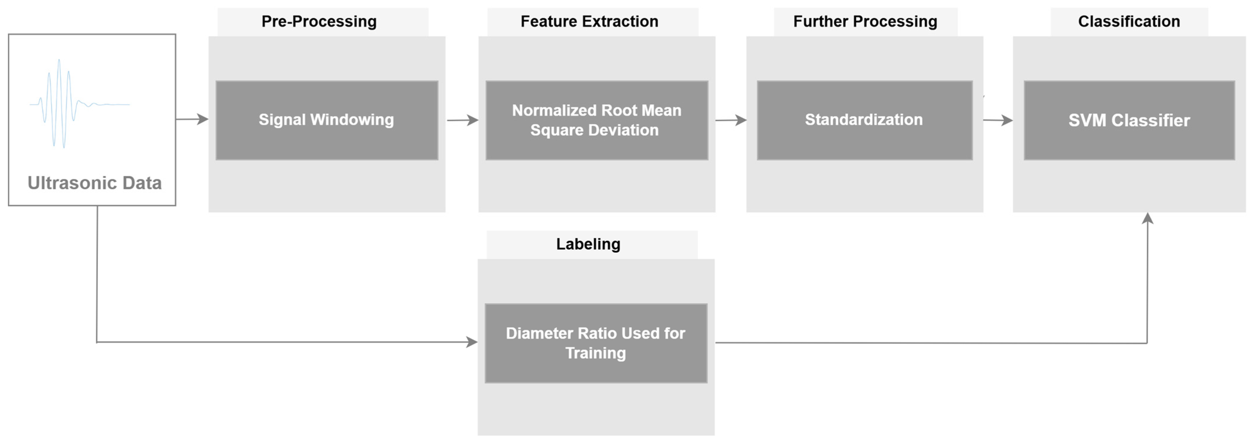
Following the described processing pipeline (Figure 8), we benchmarked 2300 algorithms by testing all windowing configurations. The results are validated using the Leave-One-Group-Out Cross-Validation (LOGO-CV). This validation method combines the benefits of standard k-fold CV with increased robustness by improving the independence between training and test data during the grouping process [13]. In LOGO-CV, groups are defined based on the damage configurations listed in Table 1, with sensor pairs grouped by each experimental setup. Since the experiment includes 8 damage configurations, this results in a total of 8 groups. In each validation cycle, one group is used as the test dataset, while the remaining sensor pairs form the training dataset.

The reconstruction of the damage location using the predicted binarized diameter ratios, as defined in Formula (4), is performed by mapping the classes representing sensor pairs affected by damage to their original diameter ratio thresholds. These thresholds are expanded by a small delta value of 0.01 to include damage that lies precisely on the perimeter of the ellipsoid, which represents the region covered by ultrasonic wave propagation between the transducer and receiver pair under investigation. The corresponding ellipsoidal regions are then plotted, and their superposition results in local maxima that indicate the reconstructed damage locations. Formula (5) describes the process of identifying the damage location by superimposing these ellipsoidal regions. Threshold $D_{th}$ is set such that the area around the local maxima is at least two-thirds higher than the lowest value in the tomogram. This ensures sufficient separation from other non-significant local maxima. Therefore, $D_{th}$ is set to 0.667 as all values are normalized to a range of 0 to 1. A more accurate threshold will be investigated in future work. Finally, centroid $C$ of the highlighted area is calculated [27], and its coordinates represent the predicted damage location.

$$\left\{\begin{array}{c}T=R_B+∆, ∆=0.01\\ A=\left({\displaystyle \sum _{s=i}^n}{T}_i\right)>D_{th}\\ \overline{x}=\underset{x_{min}}{\overset{x_{max}}{\int }}dA\ast dx/A\\ \overline{y}=\underset{y_{min}}{\overset{y_{max}}{\int }}dA\ast dy/A\\ C=(\overline{x},\overline{y})\end{array}\right.$$

(5)

$R_B$: The binarized diameter ratio as defined in Formula (4).

$T$: The tomogram representing a single ellipsoidal region associated with the investigated sensor pair.

$D_{th}$: The damage threshold set to two-thirds (0.667) of the normalized scale.

$A:$ The area of the local maximum where the predicted damage is located.

$s:$ The sensor pair under investigation.

$n:$ The total number of sensor pairs investigated.

$\overline{x}:$ The x-coordinate of the centroid of the damage location.

$\overline{y}:$ The y-coordinate of the centroid of the damage location.

$C:$ The centroid of area A, representing the location of the predicted damage.

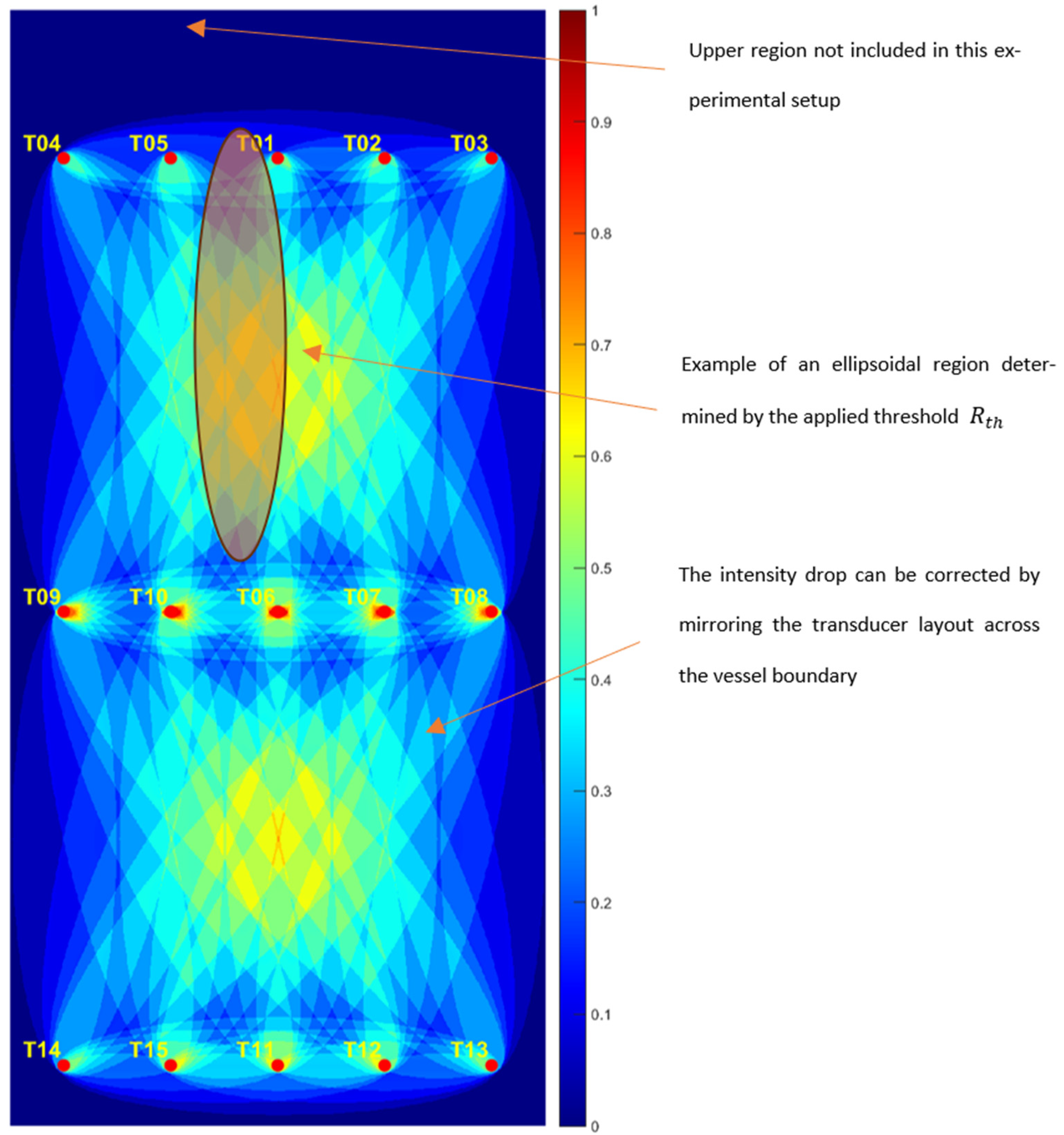
Plotting all possible ellipsoidal regions results in the tomogram shown in Figure 9. For this visualization, diameter ratio threshold $R_{th}$ is set to 0.97 to demonstrate that the localization method is capable of covering the entire area of the pressure vessel under investigation. The upper and lower regions of the vessel are not included in the scope of this experiment; therefore, no ellipsoidal regions are expected in those areas. Additionally, the left and right vertical regions show lower intensity compared to the central region. This effect is due to the simplification introduced by flattening the cylindrical geometry of the pressure vessel. This can be mitigated by mirroring the sensor transducers located on the borders to the opposite edges. However, this adjustment is not applied in this work, as the training data for the machine learning model only includes damage cases located in the central region of the vessel.

3. Results

3.1. Binary Classification Results

3.1.1. Windowing Selection

To determine the parameter configuration of the ML algorithm that delivers the best accuracy, we evaluate the algorithm described in the pipeline in Figure 8 while varying the windowing start and end data points. This results in the surface curvature shown in Figure 10. The highest accuracy is achieved by start data point 220 and end data point 564, which correspond to a time lapse of 81 μs to 246 μs after the pitch signal has been triggered.

3.1.2. Best Diameter Ratio Cutoff

A suitable binarization threshold, as introduced in Formula (4), must also be determined. To this end, the classification accuracy of the algorithm, using the windowing strategy described in the previous section, is evaluated for thresholds ranging from 0.90 to 1.00 in increments of 0.01. The results indicate that a threshold value near the center of this interval yields the highest accuracy, reaching 99.50% (

Table 2. An evaluation of the cutoff threshold applied to the diameter ratio for binarized damage classification. The classification accuracy for each of the 8 damage configurations is reported for every threshold value, along with the corresponding average accuracy.

	Accuracy in %
Damage Ratio	Damage Config 1	Damage Config 2	Damage Config 3	Damage Config 4	Damage Config 5	Damage Config 6	Damage Config 7	Damage Config 8	Average
0.90	100	100	100	100	96	100	96	100	98.75
0.91	100	98	100	100	98	100	94	100	98.25
0.92	100	98	100	100	98	100	94	100	98.25
0.93	100	98	100	100	98	100	94	100	98.25
0.94	100	100	100	100	100	100	96	100	99.50
0.95	100	100	100	100	100	100	94	100	99.25
0.96	100	100	100	100	100	100	94	100	99.25
0.97	100	100	100	100	100	100	92	100	99.00
0.98	100	100	100	98	98	100	90	100	98.00
0.99	100	100	100	100	98	100	94	100	98.75

). This corresponds to 398 sensor pairs out of a total of 400 being correctly classified. Among all damage configurations, only configuration 7 achieves less than perfect accuracy. This is due to the presence of two closely spaced damage locations, which affect the predicted diameter ratio for reversible damage $D_3$. Since $D_3$ shares many sensor paths with $D_1$, the proximity leads to overlap and interference in the signal interpretation. In this case, damage $D_1$ was more dominant as it was simulated using the heavier weight (513 g) in contrast to the lighter weight (330 g) used for $D_3$ (Table 1).

3.1.3. Visualization of Binarized Classification

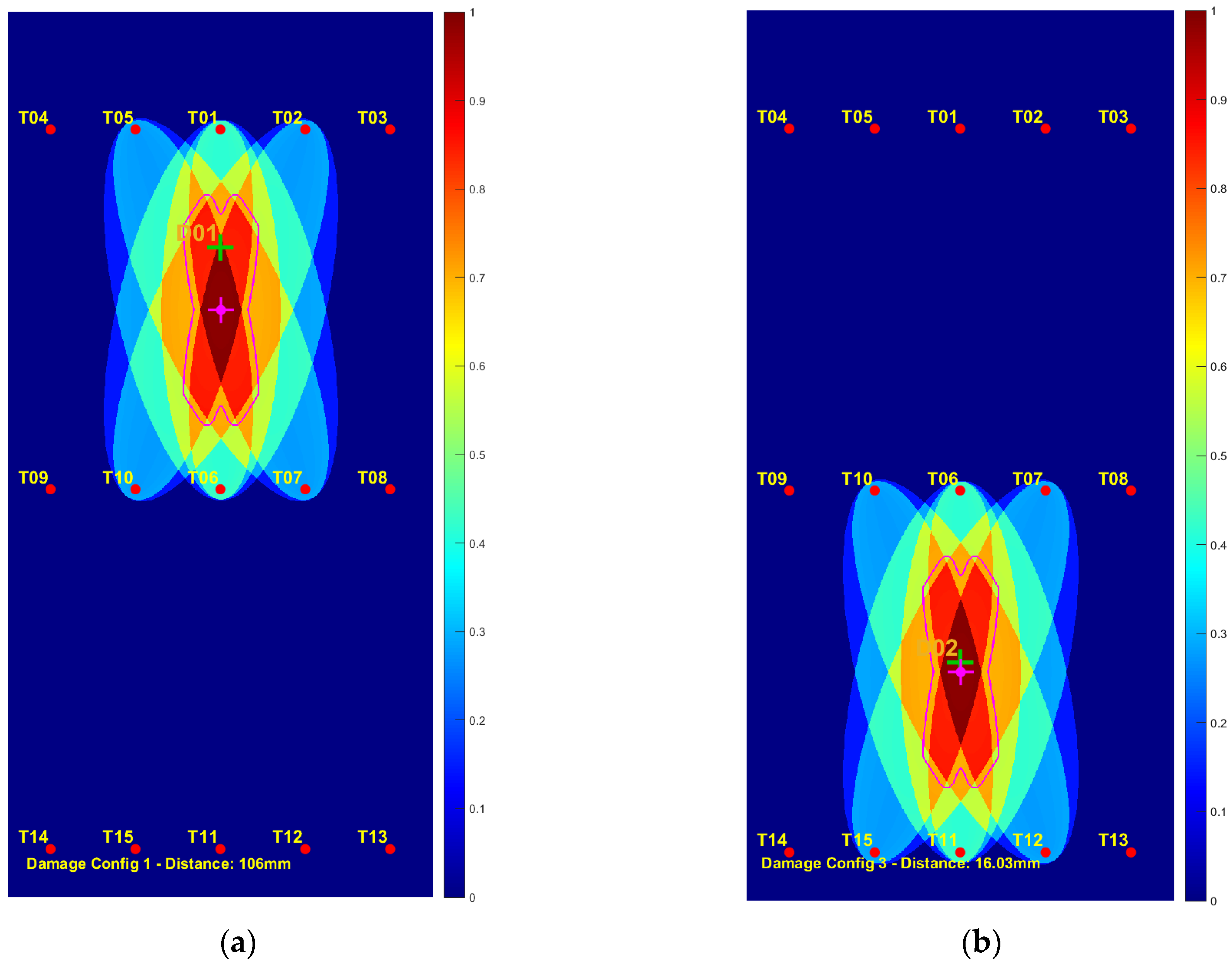
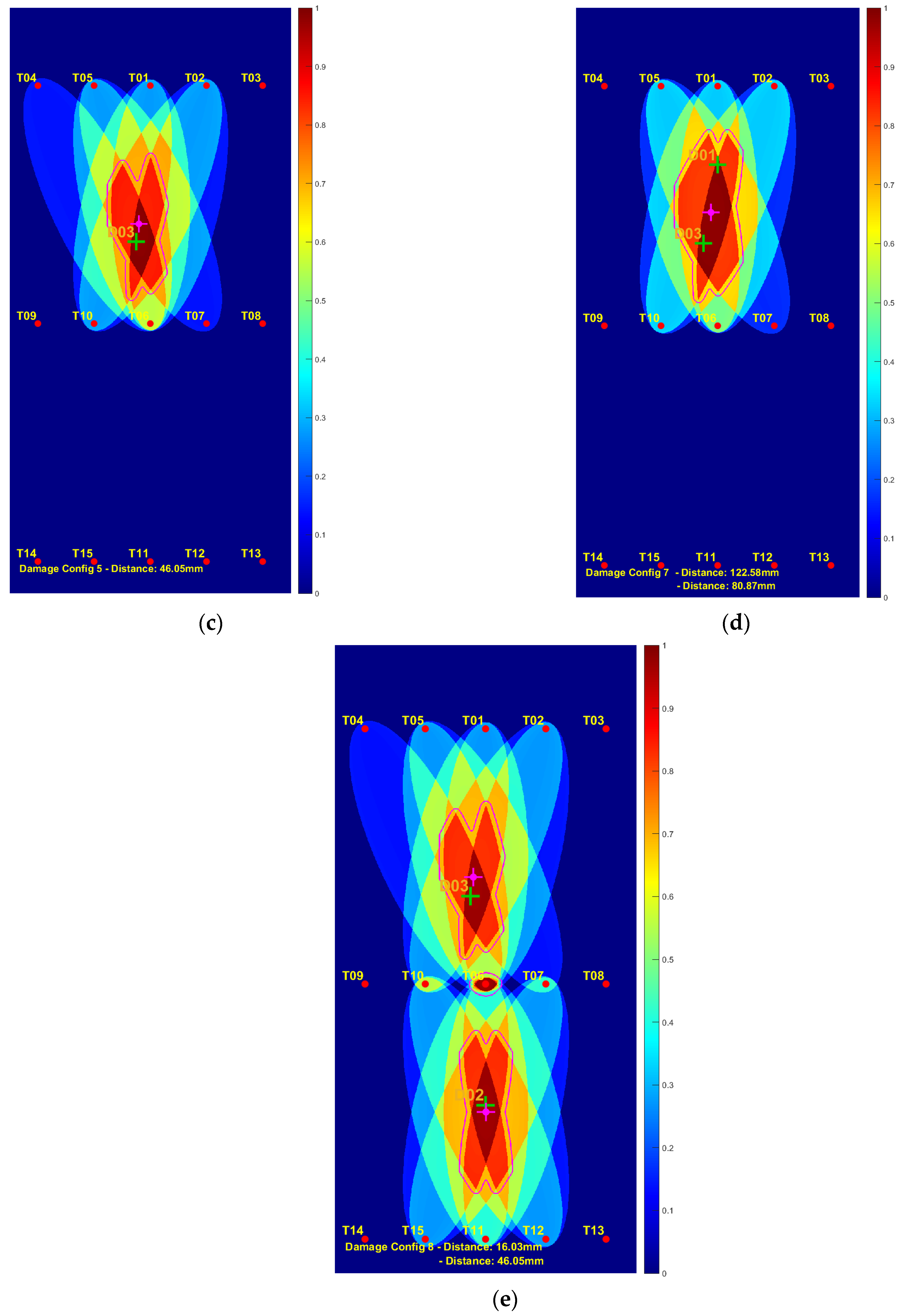
The prediction results of the machine learning model, with the parametrization that yields the highest classification accuracy, are visualized in Figure 11. The green plus symbol indicates the actual damage position, while the dot in magenta marks the predicted damage location. Damage index $i,$ as defined in Table 1, is noted by $D_i$, where $i$ varies between 1 and 3. The deviation between the predicted and actual damage positions, along with the corresponding damage configuration index, is indicated below each tomogram. This method achieves an average localization error of 60 mm.

3.2. Quantized Classification Results

3.2.1. Diameter Ratio Quantization

To achieve more accurate localization, only the edge of the ellipsoid used for triangulation is now considered when plotting the ellipsoidal region (Figure 6). Consequently, Formula (4) is modified as follows to describe the ellipsoids:

$$R_E= \left\{\begin{array}{c}{R}_{Ø},R_{th}+{∆}_{th}\ge R_{Ø}\ge R_{th} \\ 0, otherwise \end{array}\right.$$

(6)

$R_E$: The ellipsoid used to localize damage affecting the investigated sensor pair.

$R_{Ø}$: The diameter ratio, as defined in Formula (3).

$R_{th}$: Threshold for the diameter ratio that lies within the relevant interval [0.9, 1].

${∆}_{th}$: The parameter that defines the width of the ellipsoid edge set to 1 cm, ensuring coverage of the area under investigation on the studied vessel.

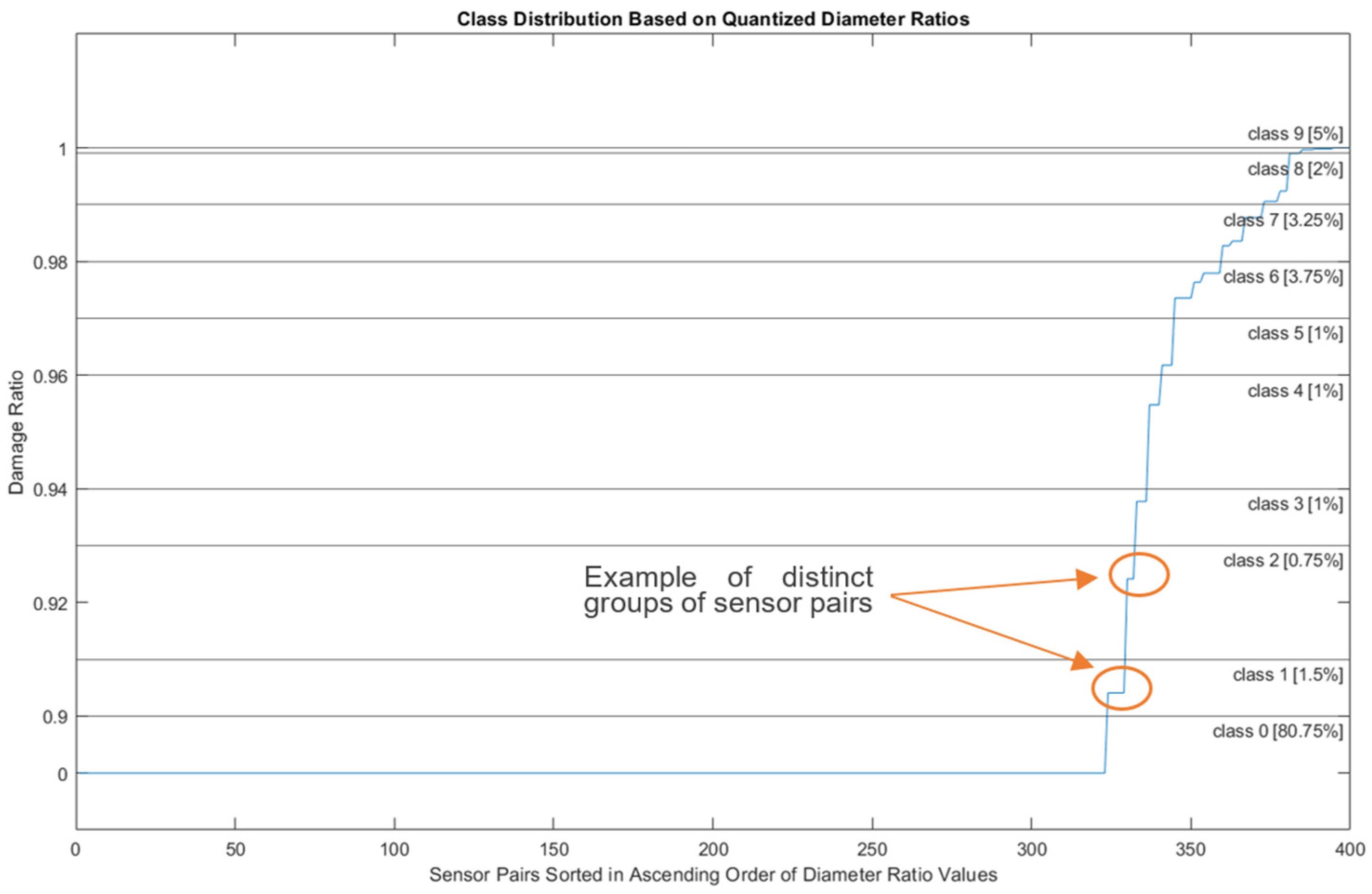
Training the proposed machine learning algorithm must be adapted to predict the diameter ratio for each sensor pair. To do this, a quantization of the diameter ratio is introduced, as shown in Figure 12. The classes are defined so that the diameter ratios of sensor pair groups fall within specific intervals, with clear separation from neighboring classes. Consequently, ten distinct classes are identified, with the number of observations per class indicated in brackets.

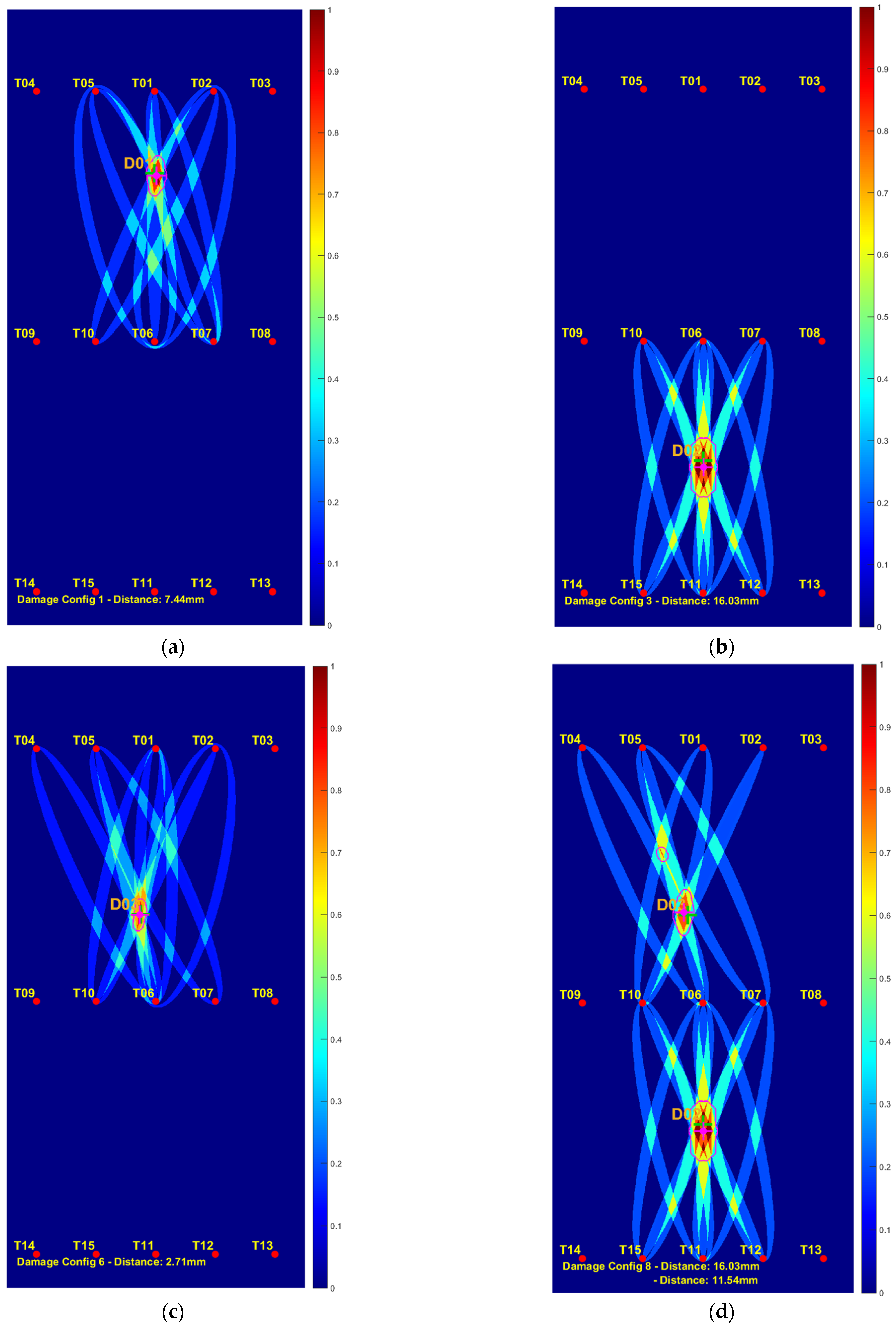
The reconstruction of the damage location using the predicted quantized diameter ratio is carried out based on

Table 3. Diameter ratio quantization mapping.

Predicted Class	0	1	2	3	4	5	6	7	8	9
Ellipsoid Diameter Ratio Recovered	0	0.90	0.925	0.945	0.95	0.96	0.975	0.98	0.985	0.999

, which reverses the quantization introduced in Figure 12. This is achieved by remapping the predicted target variable classes, that is, the prediction scores, to approximate the original diameter ratios, thereby ensuring coverage of the full range of diameter ratios within the quantized interval. The corresponding ellipsoids are then plotted, and their intersections, which result in local maxima, indicate the recovered damage locations (Formula (5)).

3.2.2. Results and Visualization of Quantized Classification

An evaluation of the machine learning model was conducted using a window that started at data point 241 and ended at data point 324, as previously determined for binarized classification (Section 3.1.1). These start and end points correspond to a time lapse of 91 μs to 131 μs after the pitch signal has been triggered. When applying a damage ratio threshold of 0.94, this parametrization results in an accuracy of 96.5%, with the lowest average localization error of 21 mm between the actual and predicted damage locations (

Table 4. An evaluation of the cutoff threshold applied to the diameter ratio for quantized damage classification. The classification accuracy for each of the eight damage configurations is reported for each threshold value, along with the corresponding average accuracy.

	Accuracy in %
Damage Ratio	Damage Config 1	Damage Config 2	Damage Config 3	Damage Config 4	Damage Config 5	Damage Config 6	Damage Config 7	Damage Config 8	Average	Localization Error in mm
0.90	96	100	98	92	92	96	84	88	93.75	30
0.91	96	100	100	98	92	98	84	94	95.00	29
0.93	94	100	100	98	92	98	84	94	95.00	26
0.94	96	100	100	98	96	100	86	96	96.50	21
0.96	94	100	98	100	96	100	86	96	96.25	23
0.97	96	100	100	98	96	100	88	98	97.00	25
0.98	96	100	100	100	98	98	88	98	97.25	20
0.99	98	100	98	100	98	98	94	98	98.00	29
0.999	100	100	100	98	98	100	94	100	98.75	66

). The predicted damage ratios are then used to reconstruct the damage positions, as shown in Figure 13. The damage ratio threshold of 0.94 yields the highest accuracy and aligns with the results obtained for binarized classification, where the same threshold also produced optimal accuracy (Table 2).

4. Discussion

The developed algorithm shows robustness against outliers. The region where ellipsoids intersect indicates the location of damage with the highest intensity. This approach ensures that, even if incorrect predictions create extra intersection points, their effect on the final damage localization is minimal because their intensities are significantly lower than those of the actual damage area. This robustness is achieved by training the model on quantized diameter ratios, which enables the estimation of approximate damage locations. In contrast, training with binarized diameter ratios only provides a binary indication of whether damage exists between a specific transducer pair. Although the localization method based on ellipsoidal regions and binarized classification results in a slightly higher average localization error (60 mm) compared to the method using quantized classification (21 mm), it has proven very effective for reliably assessing the general condition of the pressure vessel and providing a reasonable estimate of damage locations.

When grouping sensor transducer pairs, pairs that lie entirely on the sensor rings cannot be effectively trained. This is due to the lack of damage scenarios located directly on or near these sensor rings. Therefore, future experiments should consider placing damage near or on the rings to improve training coverage. On the other hand, the introduced regrouping strategy for sensor pairs helped address data imbalance. Specifically, it reduced the number of sensor pairs labeled as zero (no damage) in the selected group, from 90% down to 80%, thereby improving the learning conditions for the model. The introduced regrouping of sensors highlights the need for a further investigation of the proposed sensor arrangement. Future work should explore an equidistant placement of the transducers. Furthermore, reducing the sensor spacing may also improve the model’s accuracy. Hence, determining the optimal spacing while minimizing the number of transducers should be further investigated.

When examining Table 4, a slight effect of damage size on the model’s accuracy can be observed. This is because a larger weight causes greater changes to the surfaces of the COPV, which in turn affects how the guided waves propagate [28].

Addressing multiple incidents of damage can be considered in two cases. The first case examines the presence of damage in different areas of the vessel, as shown in Figure 11e and Figure 13d. In this scenario, the UGW signals from the upper region of the vessel are not affected by damage from the lower region due to the use of appropriate signal windowing, which filters out reflections and absorptions from other areas. The second case involves multiple cases of damage on the same vessel areas, as shown in Figure 11d. In this scenario, a superposition of the signals is assumed, since signal cancelation would result in the non-detection of damage. The complexity here mainly arises from the reflections and absorptions that occur during the propagation of UGWs between the transmitter and receiver. The applied windowing does not filter out these signal alterations because they happen within the time interval containing relevant information used to build the model’s features. This affects the model’s accuracy, as evident in Table 2 and Table 4, particularly when considering damage configuration 7.

It is worth noting that glued-on damage was used at this stage to validate the model non-destructively. This testing method is widely employed and yields results similar to those obtained with real damage [15]. However, future work will assess the model’s performance on COPVs with actual damage, such as surface cuts or drilled holes.

The validation strategy in this study has also been significantly enhanced. Instead of leaving out a single sensor pair, the evaluation is performed by leaving out one entire damage configuration out of a total of eight. Each configuration includes variations in damage severity (simulated through different weights) or different damage locations. However, future studies should investigate grouping damage positions more systematically to further improve generalization.

5. Conclusions

This paper presented an interpretable ML algorithm based on signal similarity for damage detection and localization in COPVs. The approach involves segmenting UGW signals into equal intervals, applying similarity measures, and labeling extracted features based on their proximity to damage. A cutoff is applied to sensor pairs minimally affected by damage. Unlike previous studies, this work systematically optimizes key parameters, including segmentation intervals, quantization, and cutoff values.

Experiments were conducted using a COPV equipped with 15 piezoelectric sensors, forming 105 sensor pairs. Baseline UGW signals were recorded under undamaged conditions, followed by data acquisition with reversible damage applied at different locations. The machine learning pipeline includes preprocessing in the form of windowing, feature extraction, and classification using an SVM. The algorithm with the parametrization that yields the best performance achieves 96.5% accuracy with a localization error of approximately 21 mm when using quantized classification.

Tomograms generated from the predictions indicate that the proposed method is robust against outliers and effectively reconstructs damage locations.

Despite these promising results, several limitations should be acknowledged. First, the method relies on controlled laboratory conditions and simulates reversible damage by using glued-on weights. Therefore, its performance on more complex real-world damage, such as impact-induced delaminations or drilled holes, remains to be further validated. Second, while windowing and feature extraction reduce signal complexity, guided wave propagation in composite structures is inherently sensitive to environmental and operational variations, such as temperature, load, and pressure, which may affect robustness in practical applications. Finally, the use of a single operating frequency (130 kHz) and the A0 mode provides high sensitivity to stiffness changes. However, the approach may need to be adapted when other frequencies or wave modes are considered for larger or more heterogeneous structures. Future work should therefore focus on systematically assessing the robustness of the approach while varying operational conditions and real damage scenarios. In this regard, recent studies on robust feature engineering provide valuable insights and could guide improvements in the generalizability and prediction accuracy of the proposed method [29].

References

1. Zhai, S.; Zhou, S.; Chen, S.; Yang, B.; Li, Y. Novel Defect Location Method for Pressure Vessel by Using L (0, 2) Mode Guided Wave. J. Press. Vessel Technol. 2019, 141, 010910. [Google Scholar] [CrossRef]
2. Zatar, W.A.; Nguyen, H.D.; Nghiem, H.M. Ultrasonic pitch and catch technique for non-destructive testing of reinforced concrete slabs. J. Infrastruct. Preserv. Resil. 2020, 1, 12. [Google Scholar] [CrossRef]
3. Zima, B.; Moll, J. Theoretical and experimental analysis of guided wave propagation in plate-like structures with sinusoidal thickness variations. Arch. Civ. Mech. Eng. 2023, 23, 34. [Google Scholar] [CrossRef]
4. El Moutaouakil, H.; Prager, J.; Schütze, A.; Schneider, T. Machine Learning Model Based on Signal Difference Features for Damage Localization on Hydrogen Pressure Vessel Using Ultrasonic Guided Waves. Sensoren Und Messsyst. 2024, 130–136. [Google Scholar] [CrossRef]
5. Capineri, L.; Bulletti, A. Ultrasonic Guided-Waves Sensors and Integrated Structural Health Monitoring Systems for Im-pact Detection and Localization: A Review. Sensors 2021, 21, 2929. [Google Scholar] [CrossRef] [PubMed]
6. Xiao, Q.; Li, K.; Zhang, D.; Xu, W. Security Risks in Deep Learning Implementations. In Proceedings of the 2018 IEEE Security and Privacy Workshops (SPW), San Francisco, CA, USA, 24 May 2018; pp. 123–128. [Google Scholar] [CrossRef]
7. Goodarzi, P.; Schütze, A.; Schneider, T. Comparison of different ML methods concerning prediction quality, domain adaptation and robustness. Tech. Mess. 2022, 89, 224–239. [Google Scholar] [CrossRef]
8. Tabatabaeipour, M.; Hettler, J.; Delrue, S.; Van Den Abeele, K. Reconstruction Algorithm for Probabilistic Inspection of Damage (RAPID) in Composites. In Proceedings of the 11th European Conference on Non-Destructive Testing (ECNDT 2014), Prague, Czech Republic, 6–11 October 2014; e-Journal of Nondestructive Testing. Volume 19. Available online: https://www.ndt.net/?id=16842 (accessed on 2 December 2024).
9. Hua, J.; Lin, J.; Zeng, L. High-resolution damage detection based on local signal difference coefficient model. Struct. Health Monit. 2015, 14, 20–34. [Google Scholar] [CrossRef]
10. Wang, S.; Wu, W.; Shen, Y.; Liu, Y.; Jiang, S. Influence of the PZT Sensor Array Configuration on Lamb Wave Tomography Imaging with the RAPID Algorithm for Hole and Crack Detection. Sensors 2020, 20, 860. [Google Scholar] [CrossRef]
11. Bai, L.; Velichko, A.; Drinkwater, B.W. Ultrasonic characterization of crack-like defects using scattering matrix similarity metrics. IEEE Trans. Ultrason. Ferroelectr. Freq. Control. 2015, 62, 545–559. [Google Scholar] [CrossRef]
12. El Moutaouakil, H.; Memmolo, V.; Schauer, J.; Payman, G.; Schneider, T.; Schütze, A. Feature Extraction Based On Signal Similarity for Damage Detection with Ultrasonic Guided Waves. In Proceedings of the IEEE I2MTC—International In-stru-mentation and Measurement Technology Conference, Chemnitz, Germany, 19–22 May 2025. [Google Scholar]
13. Goodarzi, P.; Schütze, A.; Schneider, T. Domain shifts in industrial condition monitoring: A comparative analysis of au-tomated machine learning models. J. Sens. Sens. Syst. 2025, 14, 119–132. [Google Scholar] [CrossRef]
14. El Moutaouakil, H.; Fuchs, C.; Savli, E.; Heimann, J.; Prager, J.; Moll, J.; Tschöke, K.; Márquez Reyes, O.; Schackmann, O.; Memmolo, V.; et al. Acquiring a Machine Learning Data Set for Structural Health Monitoring of Hydrogen Pressure Vessels at Operating Conditions using Guided Ultrasonic Waves. In Proceedings of the 10th European Workshop on Structural Health Monitoring (EWSHM 2024), Potsdam, Germany, 10–13 June 2024; Available online: https://www.ndt.net/?id=29754 (accessed on 10 December 2024).
15. Schnur, C.; Goodarzi, P.; Lugovtsova, Y.; Bulling, J.; Prager, J.; Tschöke, K.; Moll, J.; Schütze, A.; Schneider, T. Towards Interpretable Machine Learning for Automated Damage Detection Based on Ultrasonic Guided Waves. Sensors 2022, 22, 406. [Google Scholar] [CrossRef]
16. McKeon, P.; Yaacoubi, S.; Declercq, N.F.; Ramadan, S.; Yaacoubi, W.K. Baseline subtraction technique in the fre-quen-cy-wavenumber domain for high sensitivity damage detection. Ultrasonics 2014, 54, 592–603. [Google Scholar] [CrossRef]
17. Masserey, B.; Raemy, C.; Fromme, P. High-frequency guided ultrasonic waves for hidden defect detection in multi-layered aircraft structures. Ultrasonics 2014, 54, 1720–1728. [Google Scholar] [CrossRef]
18. Voß, J.; Wittkowski, R. On the shape-dependent propulsion of nano- and microparticles by traveling ultrasound waves. Nanoscale Adv. 2020, 2, 3890–3899. [Google Scholar] [CrossRef]
19. Alleyne, D.N.; Cawley, P. The interaction of Lamb waves with defects. IEEE Trans. Ultrason. Ferroelectr. Freq. Control. 1992, 39, 381–397. [Google Scholar] [CrossRef] [PubMed]
20. Saadatmorad, M.; Jafari-Talookolaei, R.-A.; Pashaei, M.-H.; Khatir, S. Damage detection on rectangular laminated com-posite plates using wavelet based convolutional neural network technique. Compos. Struct. 2021, 278, 114656. [Google Scholar] [CrossRef]
21. Dorst, T.; Schneider, T.; Eichstädt, S.; Schütze, A. Uncertainty-aware automated machine learning toolbox. Tech. Mess. 2023, 90, 141–153. [Google Scholar] [CrossRef]
22. Spuler, M.; Sarasola-Sanz, A.; Birbaumer, N.; Rosenstiel, W.; Ramos-Murguialday, A. Comparing metrics to evaluate performance of regression methods for decoding of neural signals. In Proceedings of the 37th Annual International Conference of the IEEE Engineering in Medicine and Biology Society (EMBC), Milan, Italy, 25–29 August 2015. [Google Scholar] [CrossRef] [PubMed]
23. Carrizosa, E.; Nogales-Gómez, A.; Romero Morales, D. Heuristic approaches for support vector machines with the ramp loss. Optim. Lett. 2013, 8, 1125–1135. [Google Scholar] [CrossRef]
24. MathWorks: Support Vector Machines for Binary Classification. Version R2024a. Available online: http://www.mpi-forum.org (accessed on 15 May 2024).
25. Guo, J.; Zeng, X.; Liu, Q.; Qing, X. Lamb Wave-Based Damage Localization and Quantification in Composites Using Probabilistic Imaging Algorithm and Statistical Method. Sensors 2022, 22, 4810. [Google Scholar] [CrossRef]
26. Nerlikar, V.; Mesnil, O.; Miorelli, R.; D’Almeida, O. Damage detection with ultrasonic guided waves using machine learning and aggregated baselines. Struct. Health Monit. 2023, 23, 443–462. [Google Scholar] [CrossRef]
27. Lawley, D.N. XIII. A Statistical Examination of the Centroid Method. Proc. R. Soc. Edinb. Sect. A Math. Phys. Sci. 1954, 64, 175–189. [Google Scholar] [CrossRef]
28. Bayoumi, A.B.M.; Savli, E.; Mueller, I.; Tschöke, K.; Memmolo, V.; Moll, J. Reliability Assessment of Damage Localization Techniques for Guided Wave-based Structural Health Monitoring Systems in Composite Stiffened Structures. In Proceedings of the 11th European Workshop on Structural Health Monitoring (EWSHM 2024), Potsdam, Germany, 10–13 June 2024; Volume 29. [Google Scholar] [CrossRef]
29. Zhang, X.; Ding, Y.; Zhao, H.; Yi, L.; Guo, T.; Li, A. Mixed Skewness Probability Modeling and Extreme Value Predicting for Physical System Input–Output Based on Full Bayesian Generalized Maximum-Likelihood Estimation. IEEE Trans. Instrum. Meas. 2023, 73, 2504516. [Google Scholar] [CrossRef]
Figure 1. Comparison of two types of ultrasonic damage inspection. The yellow region illustrates the propagation area of the UGWs: (a) inspection based on conventional ultrasound can only detect damage directly beneath the sensor as it lacks the waveguide structure necessary for effective wave propagation; (b) inspection based on guided wave ultrasound.
Applsci 15 09288 g001
Figure 2. UGW signals: (a) plot of the normalized pitch signal; (b) plot of the catch signal sent by transducer T1 recorded by receiver T6, where each time sample corresponds to 0.48 μs.
Applsci 15 09288 g002
Figure 3. Pictures describing the experiment setup: (a) COPV and the data acquisition system; (b) glued piezoelectric transducers and the reversible damage.
Applsci 15 09288 g003
Figure 4. The difference signal of sensor pairs T1 to T6, obtained by subtracting the baseline signal from the corresponding signal affected by damage. This results in a residual signal that indicates the presence of damage. The earliest start and latest end data points of the window are chosen to generously cover the portion of the signal influenced by the damage.
Applsci 15 09288 g004
Figure 7. Transducer pairs are divided into three groups based on their positions. The orange arrows indicate example sensor pairs belonging to each group, shown below the flattened view of the pressure vessel. Red dots represent the transducers, while blue dots indicate the locations of damage.
Applsci 15 09288 g007
Figure 8. Processing pipeline for damage classification based on signal windowing, feature extraction, standardization, and finally, SVM classification. The arrows represent the direction of the data processing.
Applsci 15 09288 g008
Figure 9. A visualization demonstrating the full coverage of the damage localization method. The red dots indicate the transducers.
Applsci 15 09288 g009
Figure 10. The surface curvature showing the change in accuracy as a function of the start and end data points.
Applsci 15 09288 g010
Figure 11. Visualization of predicted damage at different locations: (a) tomogram of damage D1; (b) tomogram of damage D2; (c) tomogram of damage D3; (d) tomogram of damage D1 and D3; (e) tomogram of damage D2 and D3.
Applsci 15 09288 g011aApplsci 15 09288 g011b
Figure 12. Distribution of training classes based on quantized diameter ratios.
Applsci 15 09288 g012
Figure 13. Visualization of the predicted damages at different locations: (a) Tomogram of damage D1; (b) Tomogram of damage D2; (c) Tomogram of damage D3; (d) Tomogram of damage D2 and D3.
Applsci 15 09288 g013