Long-Term Cotton Node Count Prediction Using Feature Selection, Data Augmentation, and Multivariate Time-Series Forecasting

Abstract

In this paper, we present an approach to performing long-term cotton node count prediction using feature selection, data augmentation, and forecasting using a multivariate long short-term memory (LSTM) model. Specifically, we used in situ measurement data that was collected from a cotton research field from Tifton, GA, USA, to perform feature selection to select the most important input measurements and enable random data generation using Gaussian distribution to increase the size of our dataset. We concatenated the generated data to create longer, usable time-series and trained a multivariate LSTM model to predict average cotton node count. Our model’s prediction results on both the training and testing data had a low RMSE of less than 3, low MAE of less than 2.5, and high $R^2$ score of at least 0.85. Our model also showed promise in accurately forecasting cotton node count in subsequent seasons via transfer learning. In particular, our transfer learned model maintained a low RMSE of less than 7.5 and MAE of less than 3.5, despite the subsequent season data having a shorter temporal scale. Moreover, we validated our results by performing hypothesis testing against a similar time-series forecasting model, namely, the gated recurrent unit (GRU) model.

1. Introduction

Recent pressures on the agriculture sector have forced farmers to increase their yield for the rapidly growing world population [1,2]. These pressures include water scarcity, a reduced labor force, increased input costs, and field challenges. However, crop monitoring efforts have been of recent interest to help predict crop growth and provide early estimations of yield [3,4]. Observing crop morphology involves examining measurable crop characteristics such as height, branches, leaves, and fruits.

Specifically, monitoring cotton crop growth in-season is imperative for early estimation of growth conditions, milestones, and yield and the prevention of disease, plant death, or plant overgrowth [5,6,7]. Cotton growth is measured by its node development, which appear along the main stem of cotton plants and produce vegetative and fruiting branches as the cotton plant grows [8,9]. Node counts are measured manually and determine crop developmental stages such as first pinhead square, flowering, and maturation [10,11]. Ideally, cotton plants develop up to 20 to 23 nodes by harvest [5]. However, aggressive environmental conditions and changes in soil health may result in significant variation in node count than the ideal range by harvest. Thus, monitoring cotton development and growth provides insight into maturation stages to estimate harvesting and yield.

Several methodologies have been explored for monitoring cotton growth, including growing degree day (GDD), data assimilation (DA), and machine learning techniques. GDD is a traditional heuristic approach of measuring crop milestones based on ambient temperature, but disregards the effects of environmental conditions and soil health on crop development [5,12]. Additionally, DA techniques typically involve combining plant observations and predictive models for forecasting, but struggle forecasting high-dimensional and nonlinear data [13,14,15]. Examples of data assimilation techniques include sequential methods, such as Kalman filtering, and variational methods, such as 3DVar and 4DVar. These methods typically use a system of equations that define system dynamics. However, cotton plants lack a system of equations that model their phenotypic development.

As a result, machine/deep learning methods have aimed to address learning the dynamics of high dimensional data for applications in crop yield forecasting and prediction. For example, AutoRegressive Integral Moving Average (ARIMA) models and recurrent neural networks (RNNs) have both been used for time-series forecasting in agriculture applications [16,17,18]. However, variants of RNNs, such as long short-term memory (LSTM) models, have been shown to have significantly lower error rates than ARIMA models, with a reduction in error rates of at least 80% [19].

Despite recent efforts in forecasting crop yield using machine learning methods, limited research has been conducted to forecast cotton node count beyond traditional heuristic methods using GDD and images. Furthermore, forecasting crop growth remains a significant challenge as crop development is heavily influenced by environmental parameters, such as precipitation and soil health. Typically, agricultural data is only collected few times per week during a few months of the growing season. While recording these characteristics periodically provides farmers and researchers with a contextualized perspective on in situ crop health, there is limited temporal length in the data, which, in turn, makes developing a short-term model insufficient for long-term and large-scale forecasting.

The contribution of our research is in the development of a long-term forecasting model to accurately predict average node count. Our developed method uses feature selection, data augmentation, and multivariate time-series forecasting of in situ field measurements. Specifically, we used long short-term memory (LSTM) networks to train a multivariate model to predict average node count. The model was trained using plant-specific measurement data collected from a cotton research field in the University of Georgia Tifton Campus in Tifton, GA, USA. The measurement data was fed into Recursive Feature Elimination (RFE), a feature selection algorithm, to select the most important measurements for predicting node count. The most important features from RFE were used to randomly generate time-series data using Gaussian distribution for long-term forecasting. Additionally, we examined our trained model’s performance on subsequent season data for generalizability via transfer learning.

The remaining sections of this paper are organized as follows: Section 2 details our methodology on collecting in situ plant measurement data, performing feature selection, generating random time-series data, and training our multivariate LSTM model for cotton node count prediction. Section 3 presents our training results for long-term cotton node count prediction, its applicability to subsequent seasonal data via transfer learning, and its validation using statistical testing against another time-series forecasting model. Section 4 discusses potential avenues of future work to improve our results. Finally, Section 5 concludes our efforts presented in this paper.

2. Methodology

2.1. Cotton Farm Details

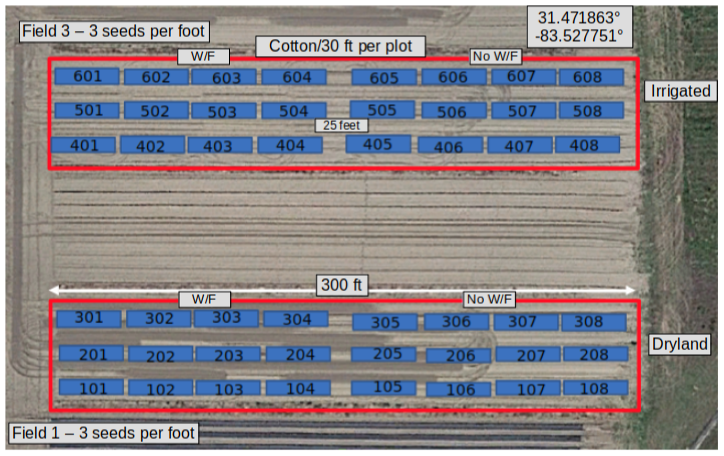
The research farm we used for data collection is located at the University of Georgia Tifton Campus in Tifton, GA, USA. The cotton plants were planted (at a rate of 3 seeds/foot) and grown during the 2023 growing season from May to October. The research field consisted of 48 plots of cotton plants, partitioned into ‘Field 1’ and ‘Field 3’. Both fields consisted of 24 plots, organized into 3 rows of 8-numbered plots each. The length of the rows was 300 feet, and each plot was 30 feet long. Field 1 contained the 100 s, 200 s, and 300 s plots and were not irrigated. Field 3 contained the 400 s, 500 s, and 600 s plots and were irrigated. Also, the first four plots of each row were naturally infested with whitefly pests. An aerial view of the farm and the plot layout is shown in Figure 1.

2.2. Cotton Data Collection

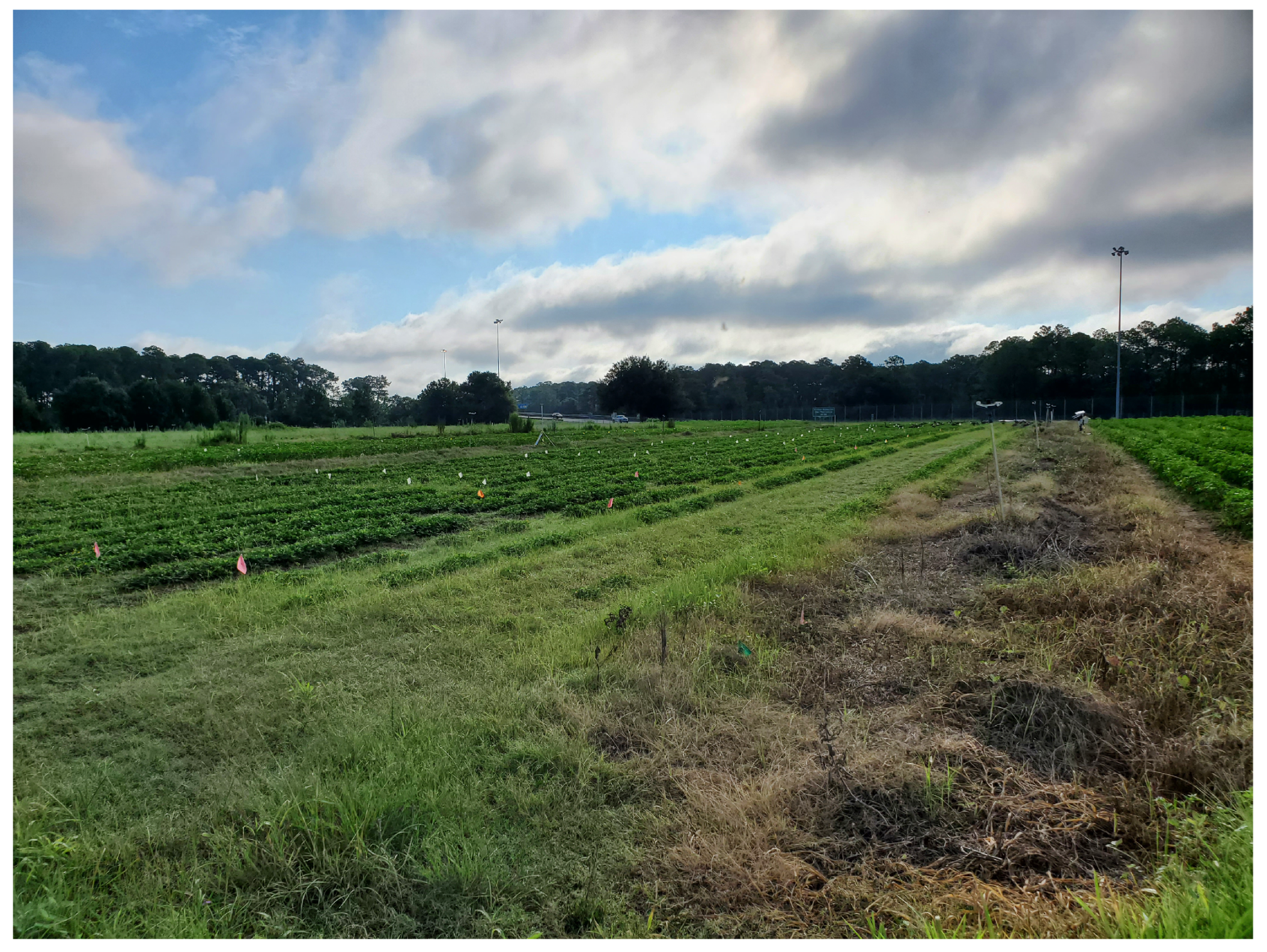
Given the size of the research field, only the 200 s and 500 s plots were selected for data collection. Within each of the 200 s and 500 s plots, 8 plants were flagged 3 feet apart from each other and on both sides of the plots. A total of 128 cotton plants were marked and served as the samples for data collection throughout the growing season. Figure 2 shows Field 3 and the marked plants with white flags.

The manual data that was collected included height, chlorophyll content (SPAD), soil moisture content, node count, boll count, flower count, nodes above the white flower, electrical conductivity, and soil temperature. The height, node count, boll count, flower count, and nodes above the white flower were measured manually. The collected data was stored in an excel file in chronological order per plot. The data was collected twice a week beginning from 14 June to 28 September prior to harvest. There were a total of 29 data collection days.

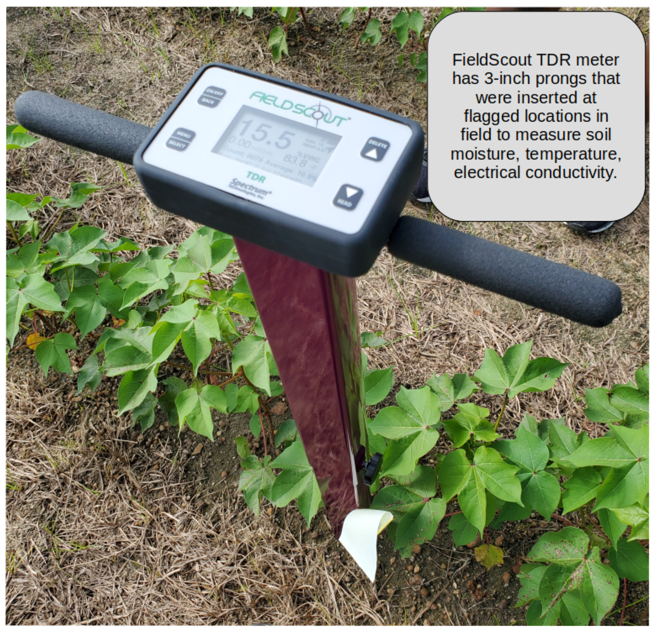
The SPAD measurement was collected using the hand-held SPAD502-Plus Chlorophyll Meter from Konica Minolta. The SPAD meter measured the chlorophyll content of the cotton plant leaves. High chlorophyll content is directly correlated to high nitrogen content with a plant, which is an indication of good plant health and development potential. Additionally, the soil moisture, soil temperature, and electrical conductivity was measured using the FieldScout TDR 350 Soil Moisture Meter from Spectrum Technologies, Inc. (Aurora, IL, USA) An example of the soil measurement using the FieldScout meter at a marked plant is seen in Figure 3.

2.3. Feature Selection

For this work, we initially selected height, SPAD, soil moisture, soil temperature, and node count measurements for our node count prediction model as these measurements directly affect node count. The other measurements, such as flower count, boll count, and node above the white flower, were not measured until later in the season. Furthermore, electrical conductivity was measured as near 0 for the entire season, so this value was not included in our training and testing datasets. Lastly, the 500 s plots succumbed to high weed pressure, which resulted in poor quality of cotton growth and yield. Thus, we focused on using the manual and sensor data collected from the 200 s plots for our model’s training set.

Given that there are many variables that are known to affect node count that were collected in the data collection process, using all of them may have been redundant and increased the complexity of the forecasting model. Thus, we aimed to reduce the number of input variables of our model using feature selection. Feature selection allowed us to identify key variables of interest that were the most important in predicting the target variable, in this case, the cotton node count, in the dataset. These identified features were then used as inputs in our model.

To achieve this, we implemented Recursive Feature Elimination (RFE) to select the important features for predicting the target variable [20]. RFE looks for a subset of features by fitting features to a selected algorithm, ranking their importance and removing the least important features recursively until the desired amount remains. We chose Random Forest Regressor (RFR) as our algorithm to choose the top three features. RFR aggregates decisions from multiple decision trees for a more accurate result.

However, while each plot had the same measurements, it is possible that each plot could have different feature importance rankings. Thus, we implemented RFE on each of the 200 s plots and compared the final important selected features and what is most common. We implemented RFE by wrapping it around the Random Forest Regressor and ran it for 500 iterations to select the top 3 features for each plot from 2023 data. The output of RFE was the feature rankings for each of the plots, either being 1 for the most important or 2 for the least important. The results for RFE are shown in

Table 1. RFE results for top 3 features for 2023 data. Height, SPAD, and soil moisture were the most important features for most plots in predicting node count using RFE in comparison to other feature combinations.

Height, SPAD, Soil Moisture	Height, Soil Moisture, Soil Temperature	Height, SPAD, Soil Temperature
201	202	204
203	206
205
207
208

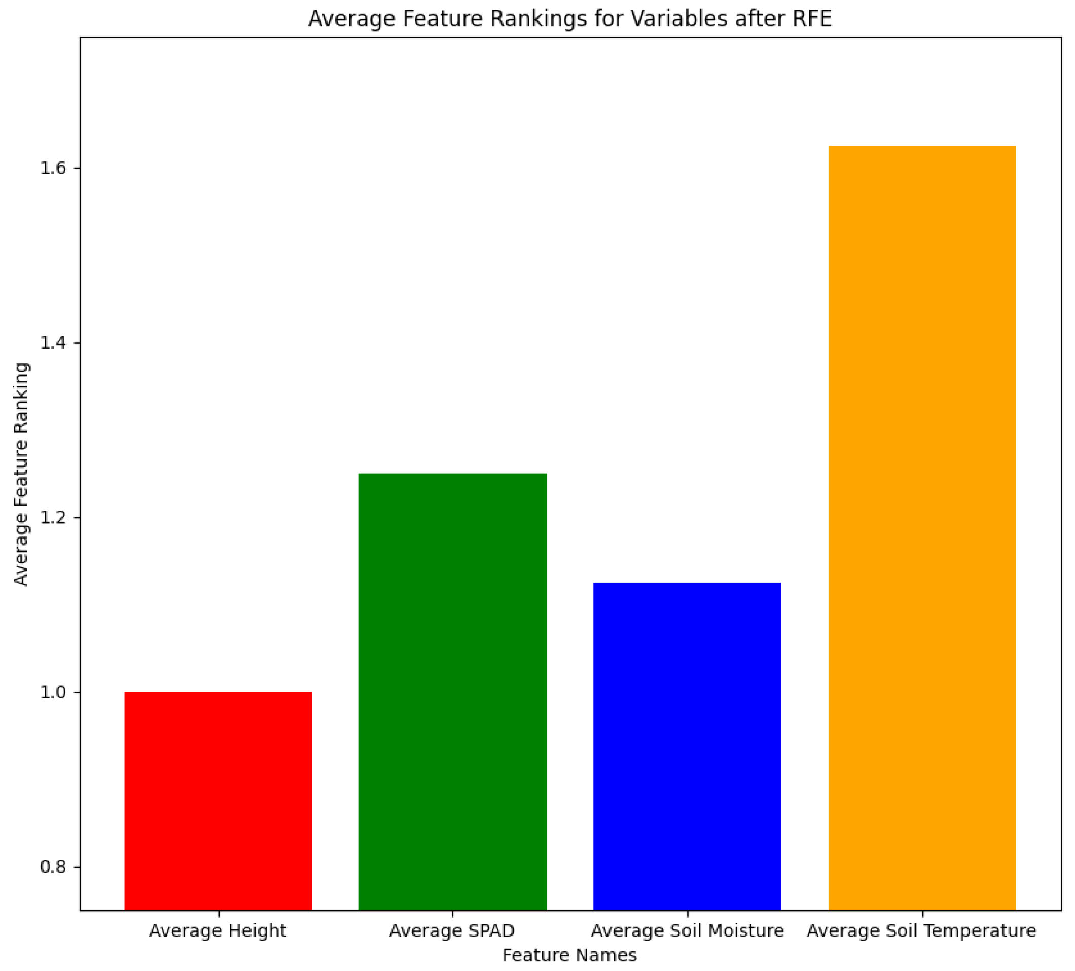
and Figure 4. As seen in Table 1, most of the 200 s plots had height, SPAD, and soil moisture as the most important features. Furthermore, we took all of the feature rankings for the 200 s plots and averaged them to visually compare the feature rankings to determine the most important variables. As seen in Figure 4, the average feature rankings for average height, SPAD, soil moisture, and soil temperature were 1, 1.25, 1.125, and 1.625, respectively. We selected the features that had the lower feature rankings, which were also average height, SPAD, and soil moisture. Thus, we used these features as input for our cotton node count prediction model.

2.4. Model Selection and Training

For cotton node count prediction, we decided to use multivariate long short-term memory (LSTM) models given that our dataset was time-series data with several measured data [21]. LSTM models are an extension of recurrent neural networks (RNNs) to address the vanishing gradient problem and storing longer sequences of data. Moreover, LSTM models have been shown to reduce the high error rates in ARIMA models and used for a variety of long-term time-series forecasting applications [19,22,23].

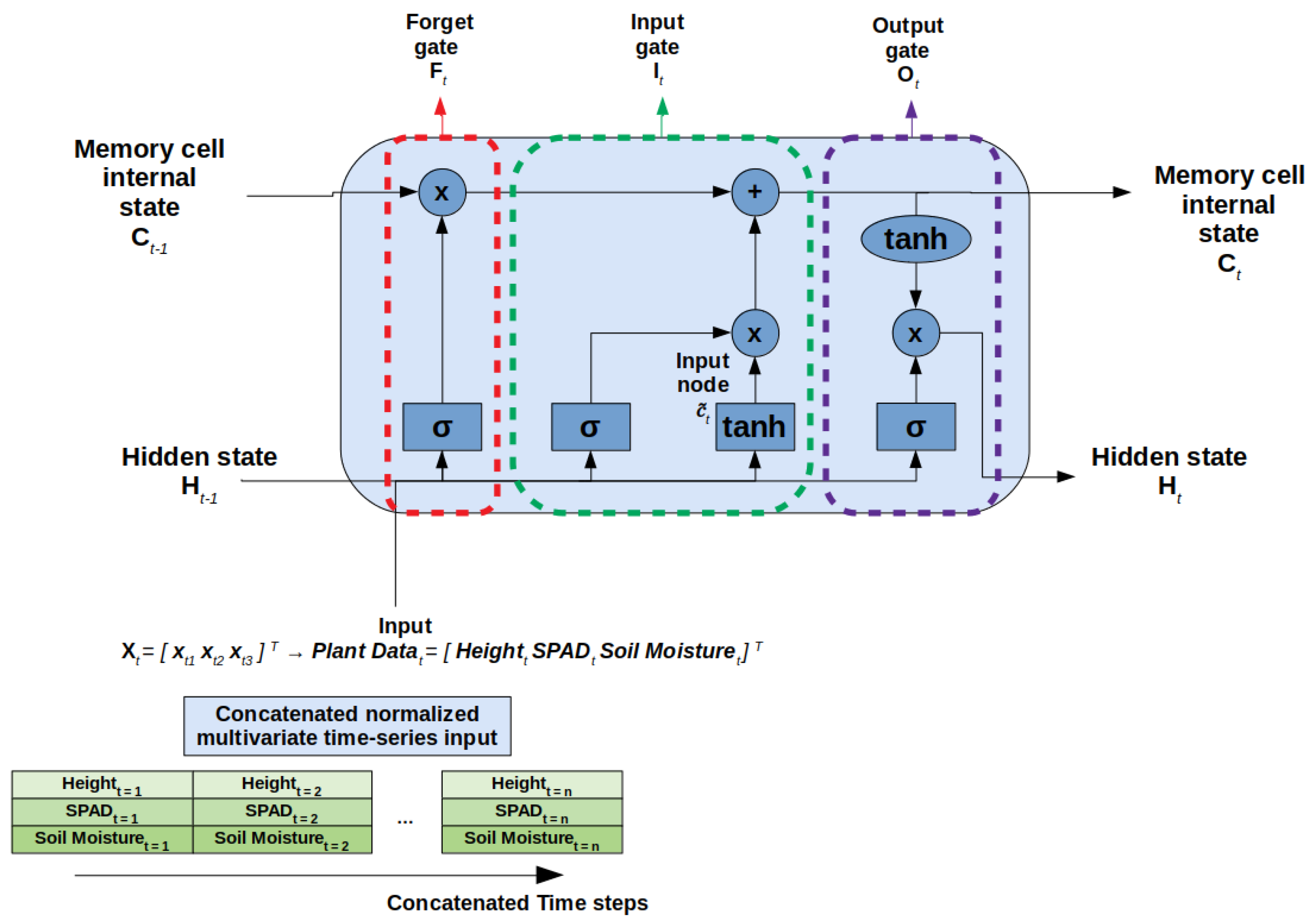
The LSTM architecture consisted of a hidden layer and was considered a gated cell. The three main gates of LSTM cells are the forget gate, input gate, and output gate. The forget gate removes information that is no longer useful. The input gate adds new useful information from the data sequence. Lastly, the output gate extracts the useful information from the current cell and is sent as final output [24].

Our multivariate LSTM model consisted of an LSTM layer and a Dense Fully Connected Layer using Keras. The final Dense layer’s activation function was modified to a sigmoid function to prevent instances of negative predictions. We modified the code from a GitHub repository from Packt (Birmingham, UK, Accessed 1 May 2024) (https://github.com/PacktPublishing/Apache-Spark-Deep-Learning-Recipes.git). Our LSTM architecture is shown in Figure 5, where the multivariate input to the LSTM cell is the cotton plant measurement data.

2.5. Data Augmentation

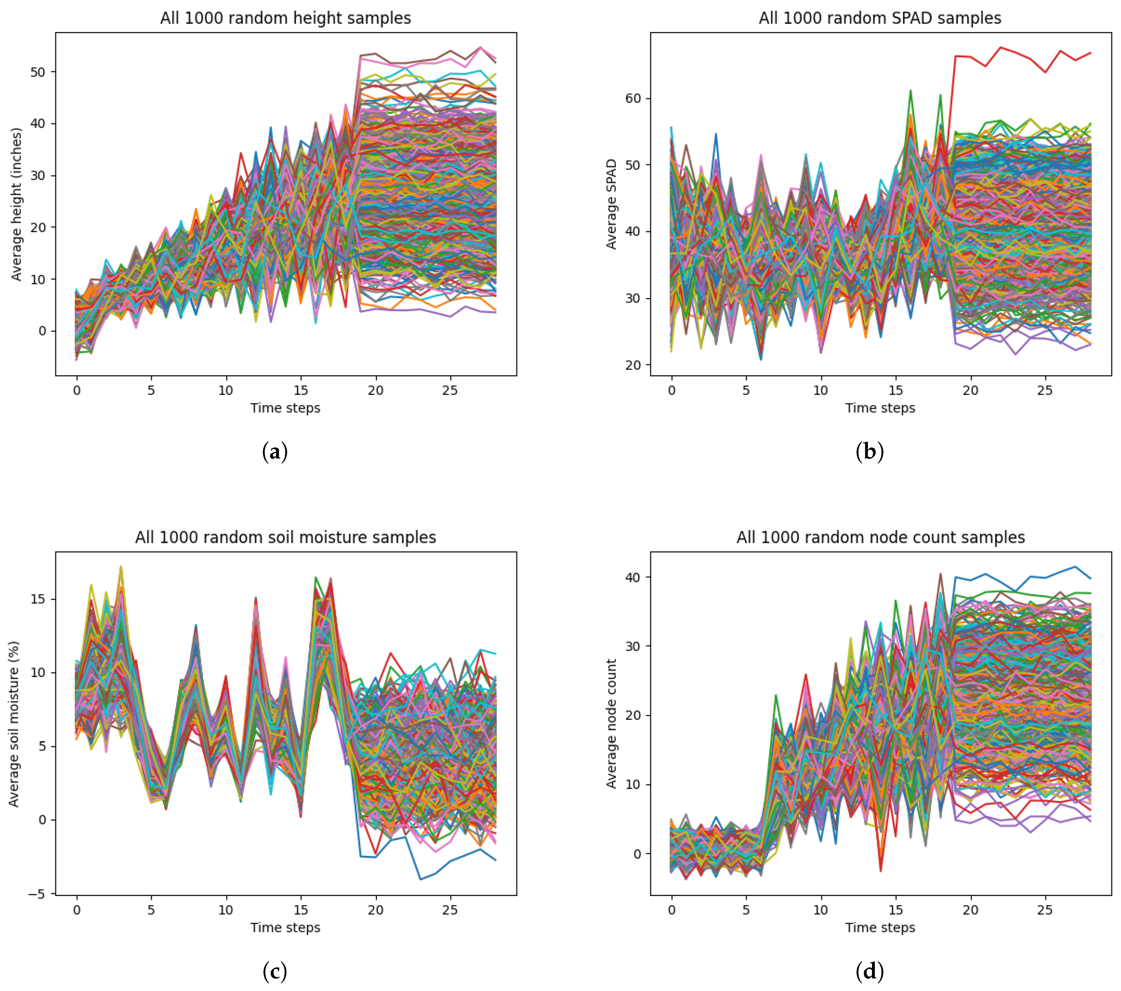
LSTM models typically perform well with longer temporal scales. Given that the temporal scale of our dataset was only 29 days, the performance of our LSTM model may have been reduce in accuracy or become overfitted. As such, we implemented data augmentation by generating random time-series data for each of the most important selected input variables from RFE and the output variable. We generated 1000 random time-series data for each variable (height, SPAD, soil moisture, cotton node count) from a Gaussian distribution for the 2023 dataset. Specifically, the average and standard deviations were calculated from all the samples from each time step. For each time step, we generated samples for height, SPAD, soil moisture, and node count based on the mean and standard deviations of that time step from the measurement data. Also, we added more variation to the final 10 time steps of each variable by adding Gaussian noise of mean 0 and standard deviation 1. This was to adjust for measurement errors during the data collection that had affected the true average and standard deviation.

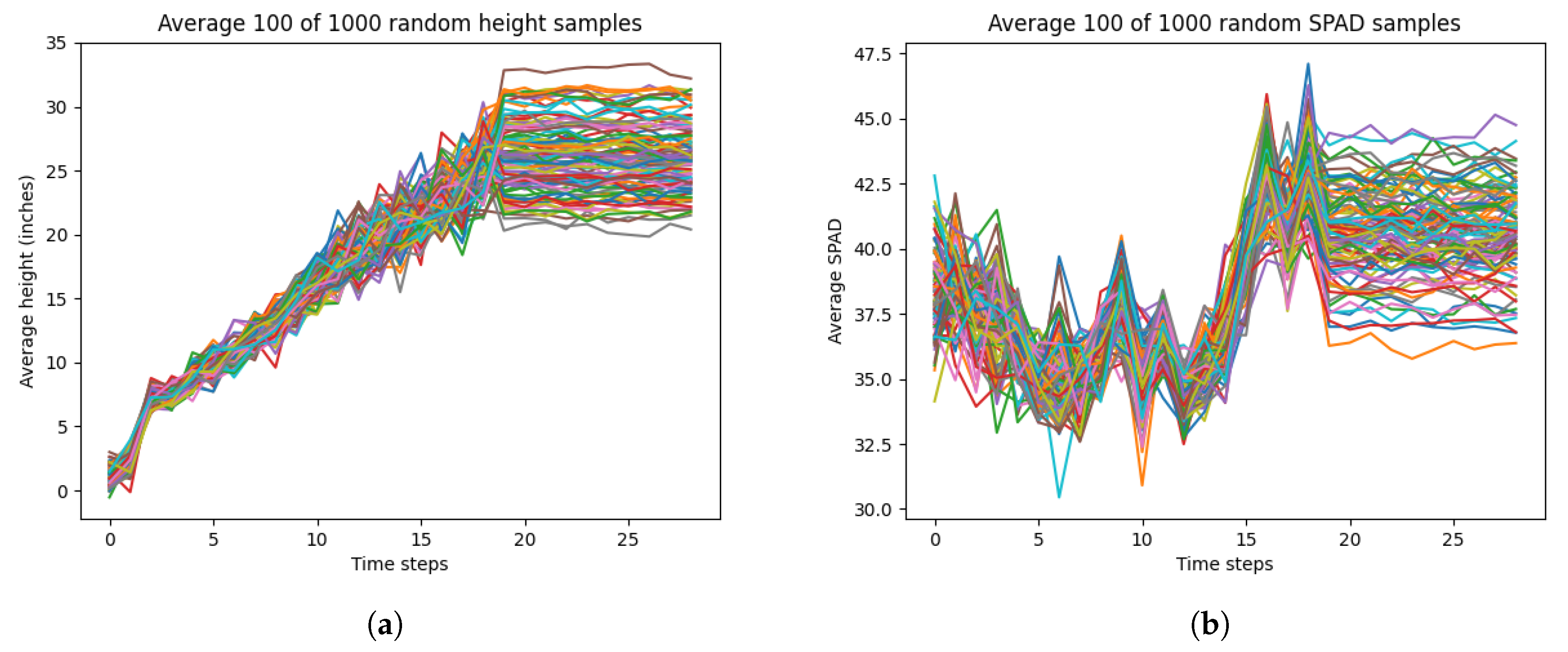
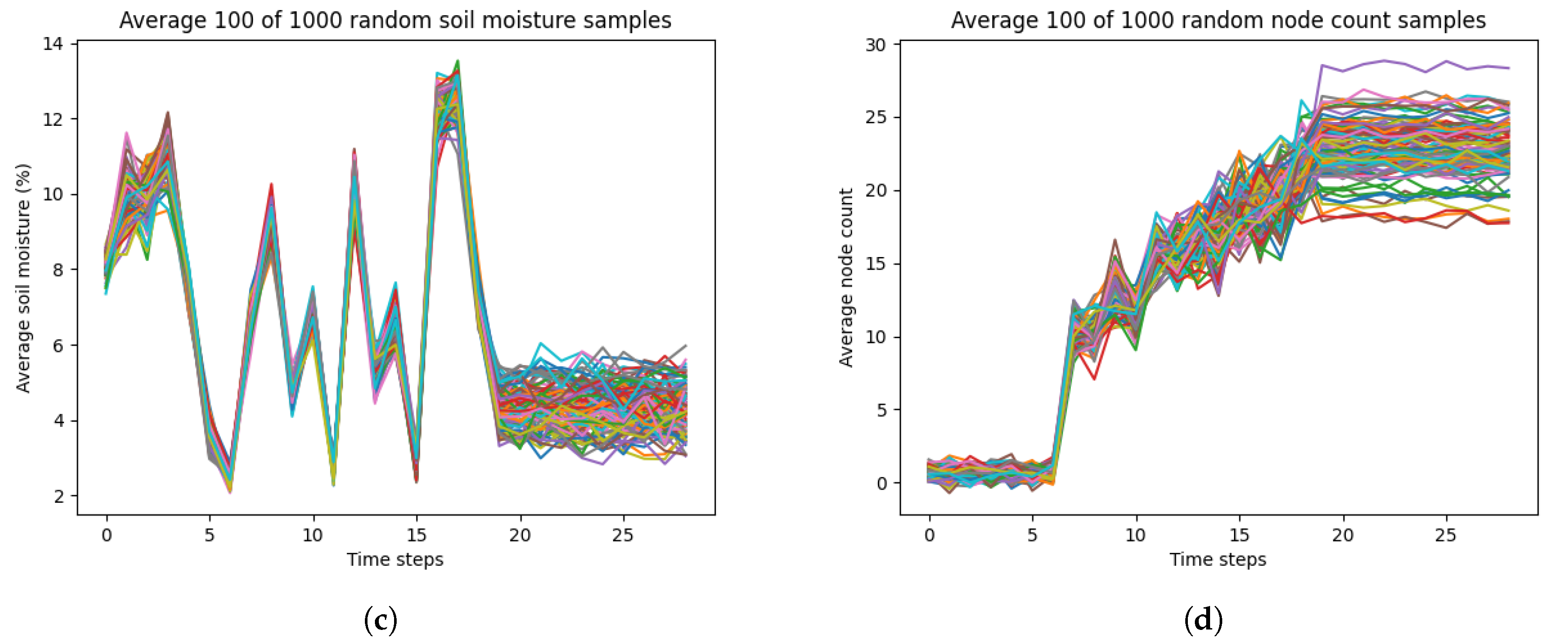
Figure 6 shows our randomly generated data. However, there was significant noise present in the randomly generated data. This was due to the variation in the standard deviation for each time step for each variable in the true measurement data. Moreover, this noise may not have been representative of true variation or growth patterns for each variable. For example, cotton node count usually reaches a maximum value of less than 30 by maturation, but the randomly generated data for node count has values that reach 40. To mitigate this noise and variability, we averaged every 10 time-series for each variable, resulting in 100 averaged time-series data. Figure 7 shows our averaged randomly generated data, which had a significant reduction of noise and mimicked realistic growth patterns.

2.6. Data Preparation for Training and Testing

To prepare our training data and further improve the performance of our LSTM model, we concatenated the 100 averaged randomly generated time-series data together to create longer, usable time-series for long-term cotton node count forecasting. Also, we combined our true measurement data with the concatenated, randomly generated data. Specifically, our training set also contained 75% randomly selected data from the original measurements from the 200 s plots. Moreover, we randomly ordered the selected true measurements with the generated data using a Python (version 3.6.9) script and the random package. The true measurement data that we randomly selected to be combined with the randomly generated time-series data included plots 201, 204, 205, 206, 207, and 208. Thus, our training set consisted of both the entire randomly generated time-series data and 75% of the true measurement data as well.

Our testing data only used the true measurement data to validate our trained model. Specifically, we used the remaining 25% plots from the true measurement data and randomly selected 50% of the true measurements in the training data. The true measurement data included in the testing set were plots 201, 202, 203, 206, and 207 only, and the time-series data was randomly ordered.

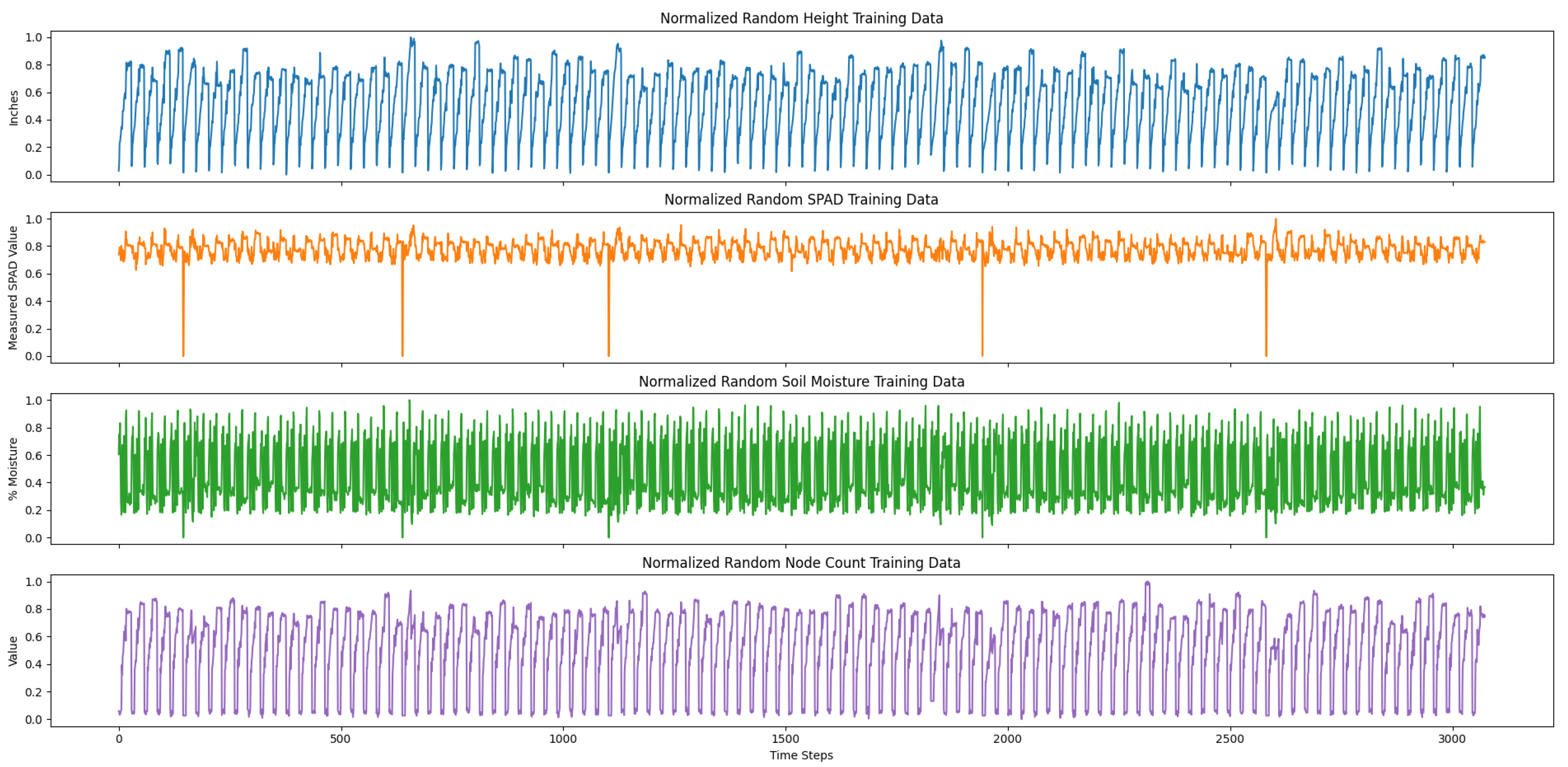
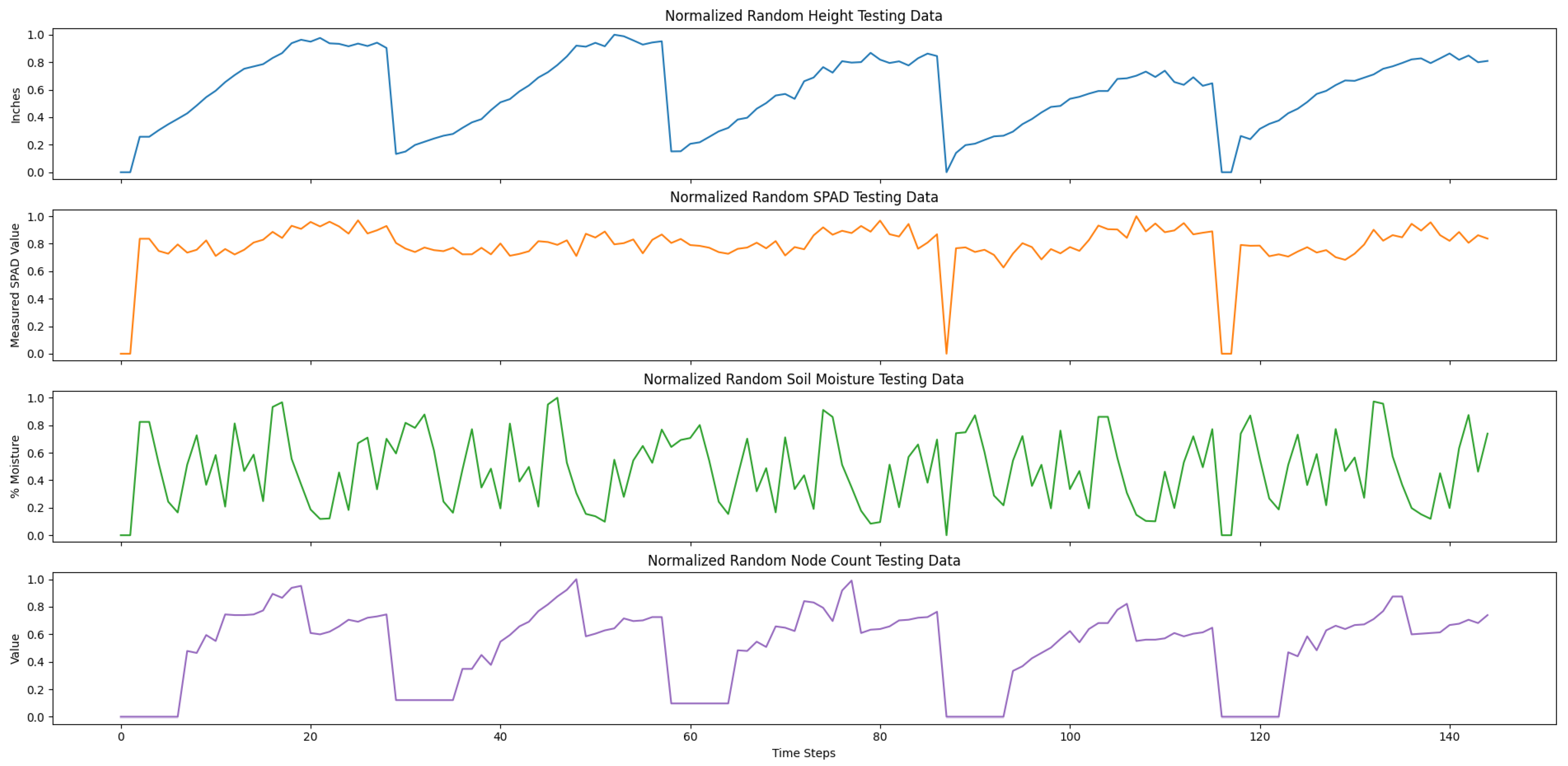
Both of our training and testing datasets were stored in comma-separated value (CSV) files. In particular, each of the columns of the CSV files were organized by time step number, date, and the averaged time-series variables. The training set consisted of 100 averaged randomly generated time-series data and a random selection of 75% of the true measurements from the 200 s plots. The training data was concatenated, resulting in 3074 time steps. The testing data consisted of select 200 s plots that were also concatenated, resulting in 145 time steps.

Lastly, to prepare our data for training, we normalized the training and testing data between a scale from 0 to 1.0 for each variable, as each variable was an inherently different unit of measure. Figure 8 and Figure 9 show our normalized, concatenated training and testing data for predicting average cotton node count using a multivariate LSTM, respectively.

2.7. Model Training

We trained a baseline LSTM model using Keras for 500 epochs using a batch size of 10, the mean squared error (MSE) as the loss function, and an Adam optimizer. The training and testing data were read into data frames for our model. The LSTM model inputs were the normalized averaged height, SPAD, and soil moisture variables. Similarly, model output was the normalized averaged node count variable. Thus, the model had 3 units as input and 1 unit for output.

2.8. Model Evaluation

The model’s original prediction results were also normalized. We rescaled the normalized results to the original scale to evaluate the model’s accuracy with the same training data and testing data. Specifically, we evaluated the results using four common time-series forecasting error measures, namely, MSE, root mean squared error (RMSE), mean absolute error (MAE), and $R^2$ score, which was the coefficient of determination [25].

We defined MSE as

$$MSE={\displaystyle \frac{1}{n}}\sum _{i=1}^n{(y_i-\widehat{y_i})}^2,$$

(1)

where $y_i$ is the true observed value and $\widehat{y_i}$ is the predicted observation from our trained model. Ideally, MSE should be low and near 0 for a well-trained, accurate model. Also, we defined RMSE as

$$RMSE=\sqrt{MSE}.$$

(2)

Evaluating RMSE is beneficial as it determines the error rate in the same units as the target variable, in this case, the cotton node count. Ideally, RMSE should also be low and near 0 for a well-trained, accurate model. Furthermore, we defined MAE as

$$MAE={\displaystyle \frac{{\sum }_{i=1}^n|y_i-\widehat{y_i}|}{n}}.$$

(3)

MAE is a common forecast error measure in time-series analysis and is also in the same scale and units as the target variable, in this case, the cotton node count. Ideally, MAE should also be low and near 0 for a well-trained, accurate model.

Lastly, we defined $R^2$ score, also known as the coefficient of determination, as

$$R^2(y_i,\widehat{y_i})=1-{\displaystyle \frac{{\sum }_{i=1}^n{(y_i-\widehat{y_i})}^2}{{\sum }_{i=1}^n{(y_i-\overline{y_i})}^2}},$$

(4)

where $\overline{y_i}={\displaystyle \frac{1}{n}}{\sum }_{i=1}^n{y}_i$. This metric is also commonly used as a forecast error measure in time-series analysis. The $R^2$ score represents the proportion of variance in an output variable that is explained by the input variables of a trained model. Moreover, this metric provides an indication of how well a model is able to predict new samples of data based on this proportion of variance. Ideally, the $R^2$ score should be positive and near 1.0 for a well-trained, accurate model.

We used sklearn’s metrics package to determine the aforementioned metrics between our prediction results and true values.

2.9. Transfer Learning

We also examined the performance and generalizability of our trained model on subsequent seasonal data via transfer learning. Subsequent growing seasons may have a variety of environmental factors that affect cotton growth, such as new fields, or changes in soil health, pests, weeding, diseases, and precipitation. As such, the data collected was similar yet different to the original dataset of the current season. Testing our trained model on subsequent seasonal data may have resulted in inaccurate predictions in cotton node count due to the inherent differences between the source data from 2023 and the target data from 2024. Moreover, training a new model from scratch for each season of data is computationally expensive. As such, transfer learning offers a time-effective method for a trained model to learn new data for a target task that is similar to the source task.

In this case, the source task was predicting cotton node count from the 2023 growing season; the target task was predicting cotton node count from the 2024 season. In the 2024 growing season, the cotton plants were grown in a research field in Tifton, GA. There were two rows of plants selected for data collection, namely, the 400 s and 500 s plots, for a total of 16 plots. Within each of the 16 plots, 8 plants were marked and flagged for data collection. There were a total of 10 data collection days and the same measurements were selected and used for data collection.

We also repeated the same feature selection technique for identifying the most important input variables for the 2024 growing season. The results of the feature selection an be seen below in

Table 2. RFE results for top 3 features for 2024 data. Height, SPAD, and soil moisture were also the most important features for most plots in predicting node count using RFE in comparison to the other feature combinations during the 2024 growing season.

Height, SPAD, Soil Moisture	Height, Soil Moisture, Soil Temperature	Height, SPAD, Soil Temperature	SPAD, Soil Moisture, Soil Temperature
401	402	407	408
501	403	502
503	404	507
504	405	508
505	406
506

, where the most important measurements for predicting cotton node count were also height, SPAD, and soil moisture. As such, we also used these variables for generating time-series data as well.

We implemented data augmentation to increase the size of the 2024 dataset for long-term cotton node count prediction. We used the same methodology to generate the time-series data by determining the mean and standard deviation for each time step of the true measurement data and then generated time-series data using Gaussian distribution for each time step, based on its mean and standard deviation. We also took the average of every 10 time-series datum to reduce noise, stored the data in a CSV file to be read as a dataframe, and normalized the data for training. A total of 100 time-series data were generated from the 2024 measurement data.

Additionally, the training set contained the 100 randomly generated time-series data along with 10 plots selected from the original 2024 data from both the 400 s and 500 s plots. The testing set contained the remaining 6 plots not selected for the training set. We also used a script to randomly order the selected true measurement data with the randomly generated data using Python’s random package. Specifically, the true measurement data included in the training set were plots 401, 402, 403, 404, 405, 406, 407, 408, 507, and 508. The true measurement data included in the testing set were plots 501, 502, 503, 504, 505, and 506. 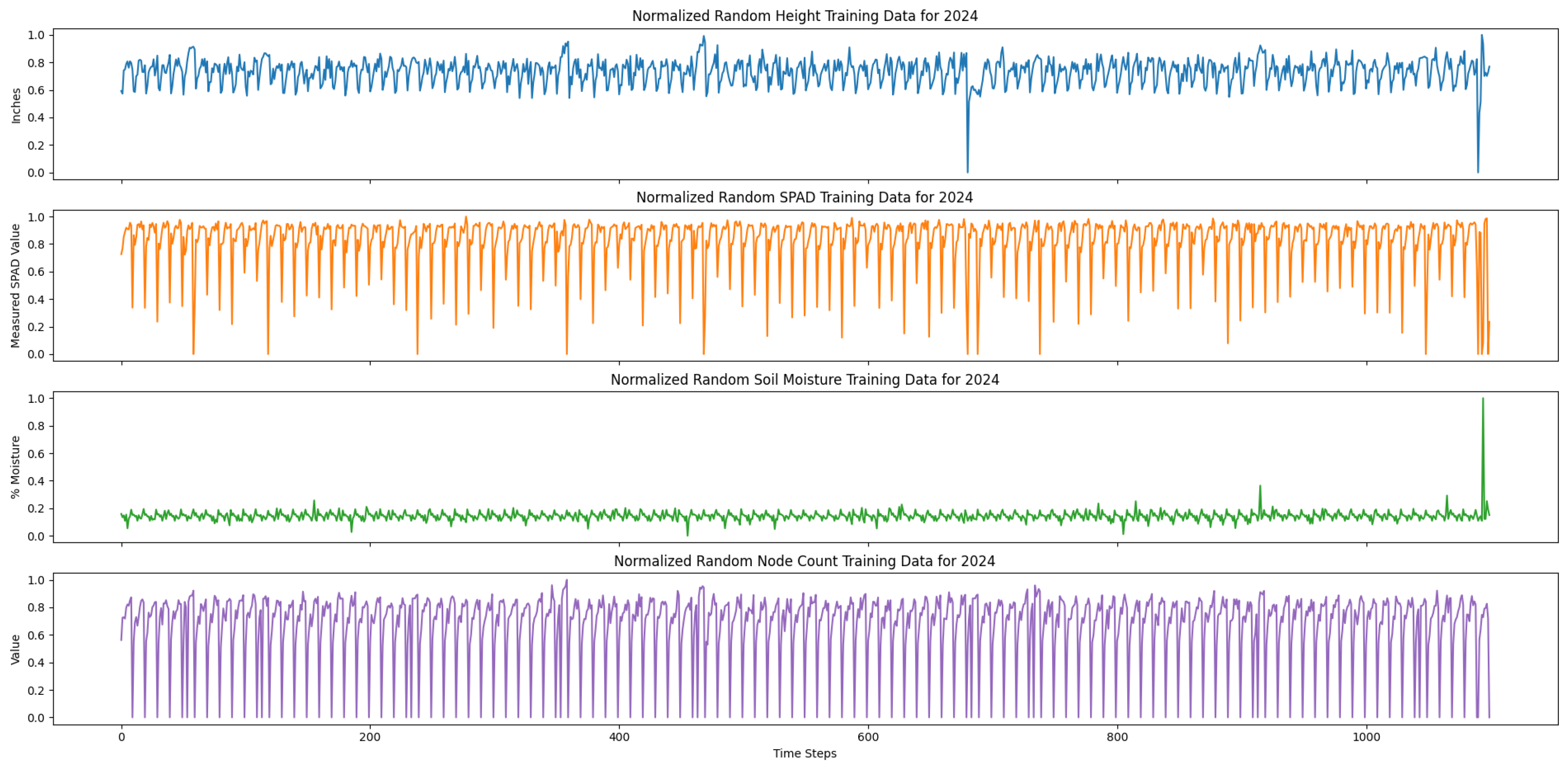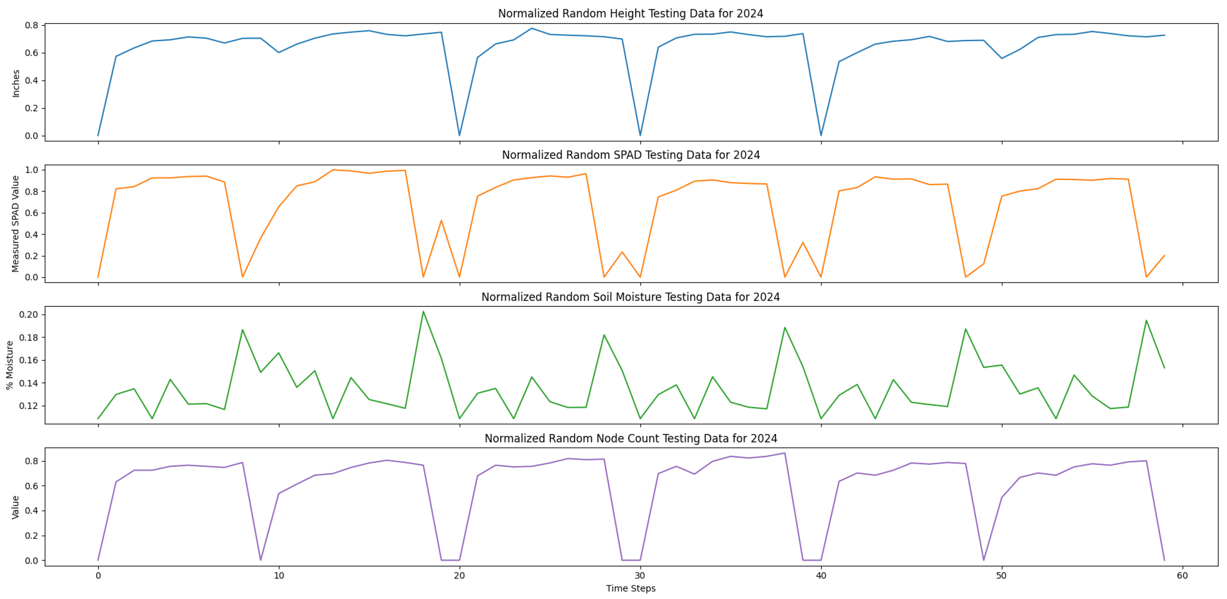Figure 10 and Figure 11 show the normalized, concatenated training and testing sets for transfer learning.

We evaluated the model performance before and after transfer learning using the same metrics presented in Section 2.8. A summary of our methods is shown in Figure 12.

3. Results

3.1. Evaluation and Prediction Results of the Trained Model

We examined our trained LSTM model’s performance on the same training data as well as the testing data.

Table 3. Evaluation of our trained LSTM model on the same training data.

Metric	Value
MSE	6.267
RMSE	2.503
MAE	1.973
$R^2$ Score	0.918

and

Table 4. Evaluation of our trained LSTM model on the testing data.

Metric	Value
MSE	8.028
RMSE	2.833
MAE	2.293
$R^2$ Score	0.8572

show the model’s performance on both the same training and testing sets, respectively. As shown in Table 3, the error rates were low and near 0. Additionally, the $R^2$ score was also high and near 1. Similarly, Table 4 also shows low error rates near 0 and a high $R^2$ score of over 0.85, indicating that the variance in the observations was similar to the true values.

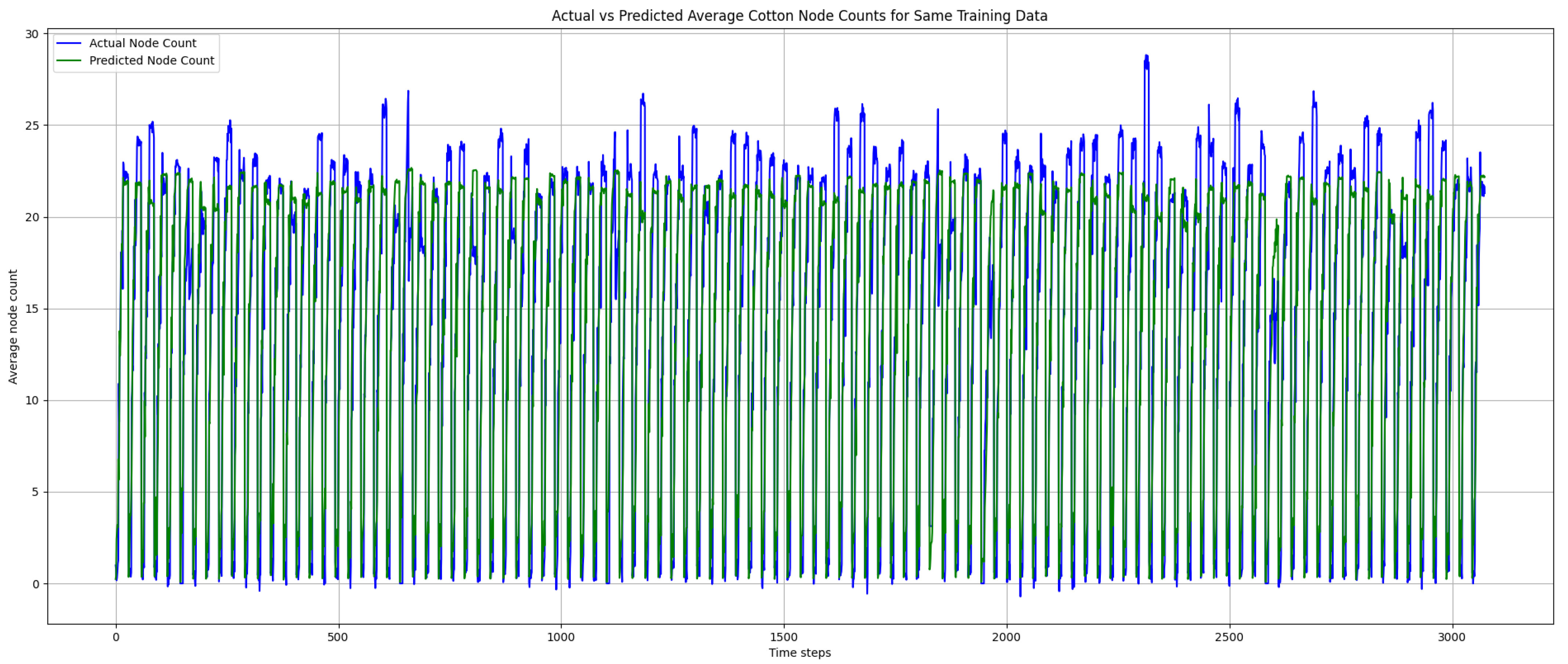
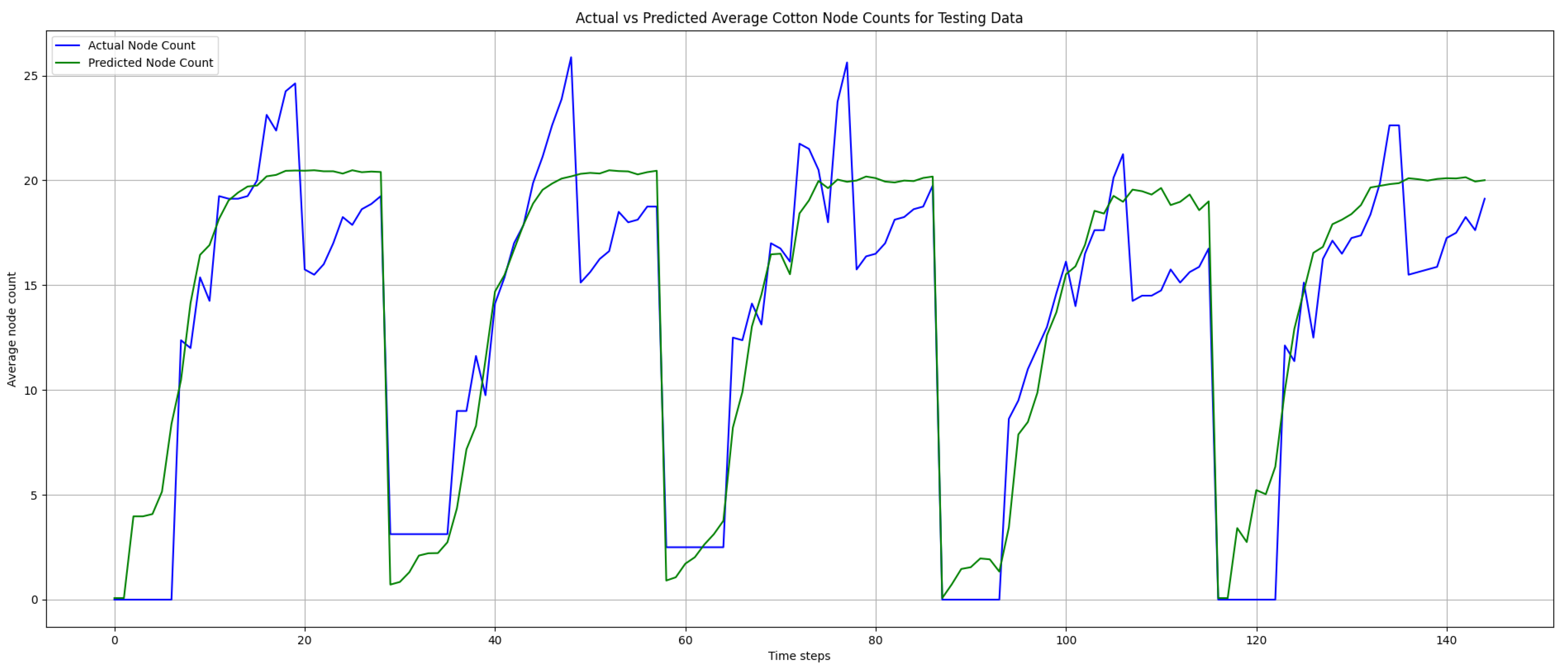
Figure 13 and Figure 14 below show the prediction results on the training and testing data, respectively. In Figure 13, the prediction results follow the true values closely, indicating that the trained model was not overfit. However, there were some instances where the prediction result did not reach the peak true node count values, which contributed to the elevated error rates. As shown in Figure 14, the prediction results also followed the true node count values closely. Additionally, there were some instances where the predicted node count over- or under-estimated the node count as well, which contributed to the elevated error rates. As shown in Figure 13 and Figure 14, there were no negative predictions, which was attributed to the use of sigmoid as the activation function in our trained model.

3.2. Transfer Learning Results for 2024 Data

We first examined our trained model’s performance on the 2024 testing dataset before the transfer learning. The source task was to predict cotton node count for the 2023 data. The target task was to predict cotton count for the 2024 data. Given that the fields and growing seasons were different, this shows that there may have been inherent differences between the growing seasons and source and target tasks. To test this difference, we examined the pretrained model performance on the target task. Ideally, the performance metrics of the model on the target task before transfer learning needed to be significantly worse than the source task. This would have justified implementing transfer learning.

Table 5. Evaluation of our trained LSTM model on the 2024 testing data before transfer learning.

Metric	Value
MSE	51.94
RMSE	7.207
MAE	4.381
$R^2$ Score	0.176

presents the performance of our pretrained LSTM model on the 2024 testing set.

Given that the performance metrics on the target task were significantly worse than those shown in Table 4, we implemented transfer learning. We loaded the pretrained model, fed it our 2024 training data, and trained the model for 500 epochs with a batch size of 2, given that the temporal scale per plot was only 10 days, and granted the model more training time to learn the target data.

Table 6. Evaluation of our trained LSTM model on the 2024 testing data after transfer learning.

Metric	Value
MSE	53.319
RMSE	7.302
MAE	3.387
$R^2$ Score	0.401

presents the model performance on the target task after transfer learning.

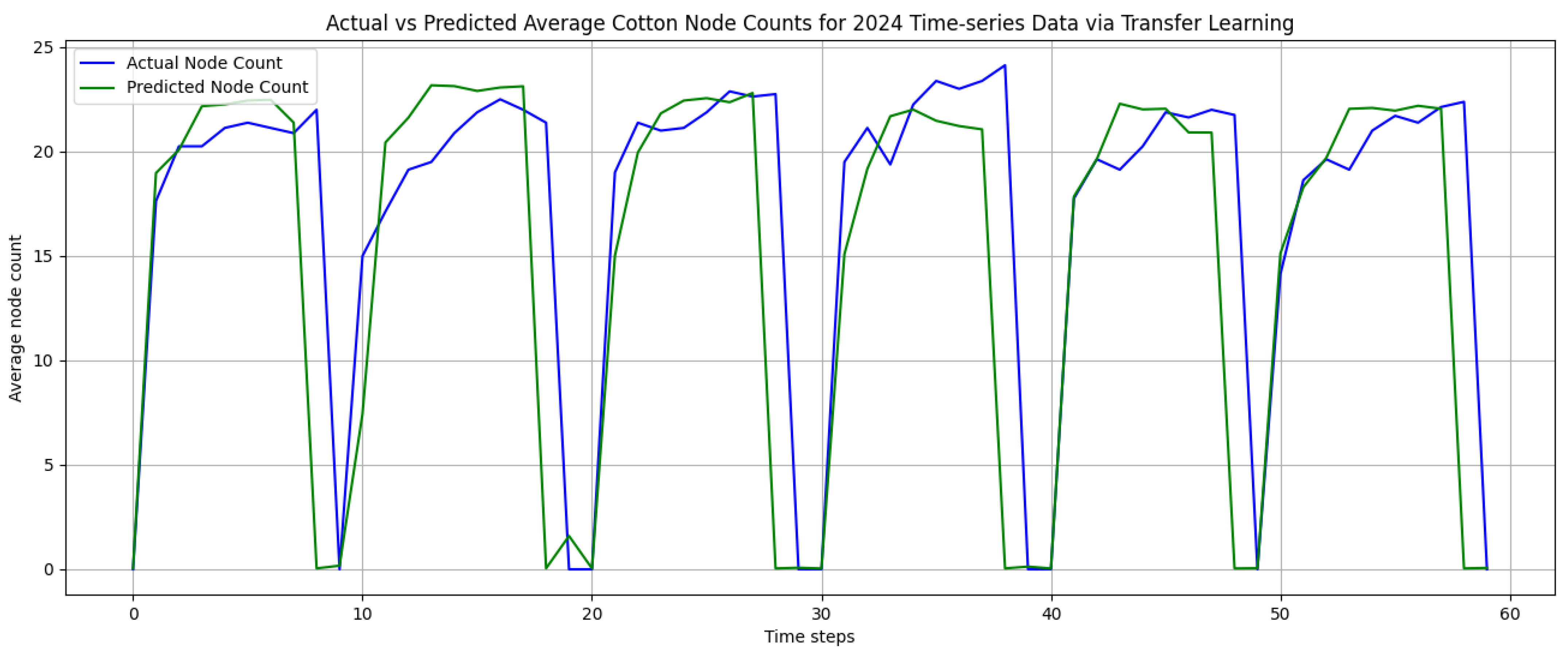
As seen from Table 6, the MAE decreased and the $R^2$ score improved and increased to 0.40, indicating that after transfer learning, model showed improved prediction in new instances of the target task. Moreover, there appeared to be a slight lag in the prediction results, attributed to the elevated MSE. This was due to the 2024 dataset having a significantly shorter temporal scale than the 2023 dataset. Figure 15 below shows the prediction results of the transfer learning model on the target task testing set. The prediction results closely followed the true randomly generated 2024 time-series testing data. Also, there were minimal over-estimations of cotton node count predictions.

3.3. Statistical Testing of Our LSTM Model with GRU

To validate our LSTM results, we tested whether they were statistically different from those of another time-series forecasting model, namely, the gated recurrent unit (GRU) model. GRUs share similarities with LSTMs in using gated cells but differ in that they lack an output gate, have fewer parameters, and generally enable more efficient training. Despite these architectural differences, our goal was to determine whether the LSTM model produced statistically different results compared to GRUs. Specifically, we compared the RMSE and $R^2$ scores on the same dataset to assess whether any observed differences stemmed from GRU’s architectural features or were simply due to random variation.

In this experiment, we trained and tested both the LSTM and GRU models five times each using Keras, with 500 epochs, a batch size of 2, mean squared error (MSE) as the loss function, and the Adam optimizer. Each model consisted of a single LSTM or GRU layer followed by a Dense layer with a sigmoid activation function to prevent negative predictions. Both models were trained and tested on the same dataset in each run and, because of the stochastic nature of training, each produced slightly different results. For each run, we recorded the error metrics (RMSE, MSE, and MAE) as well as the $R^2$ score.

We focused on assessing whether the mean RMSE and mean $R^2$ scores differed significantly between the two models.

Table 7. RMSE of both LSTM and GRU models after training both five times each.

Training and Testing Iteration	RMSE of LSTM	RMSE of GRU
1	2.49975	2.802455
2	2.488673	2.915961
3	2.819261	2.471719
4	2.77587	2.780504
5	2.816925	2.469876

and

Table 8. $R^2$ score of both LSTM and GRU models after training both five times each.

Training and Testing Iteration	${\mathit{R}}^2$ Score of LSTM	${\mathit{R}}^2$ Score of GRU
1	0.888886	0.860347
2	0.889869	0.848805
3	0.858667	0.891364
4	0.862983	0.862526
5	0.858901	0.891528

present the RMSE and $R^2$ values obtained from five independent training and testing runs for both LSTM and GRU. Although the values appeared close, we sought to determine whether these differences were statistically significant. To this end, we performed a two-tailed, paired t-test, as the two models were evaluated on the same dataset across matched runs.

We formulated our two-tailed, paired t-test for RMSE as follows. Let ${\mu }_1$ be the population mean of ${\text{RMSE}}_{LSTM}$ and ${\mu }_2$ be the population mean of ${\text{RMSE}}_{GRU}$. We defined the difference in population means as ${\delta }_{RMSE}={\mu }_1-{\mu }_2$. For our first hypothesis test, we defined our null and alternative hypotheses for testing the difference between the RMSE population means to be

$$H_0:{\delta }_{RMSE}=0,$$

$$H_A:{\delta }_{RMSE}\ne 0.$$

Similarly, we formulated our two-tailed, paired t-test for $R^2$ as follows. Let ${\mu }_1$ be the population mean of $R_{LSTM}^2$ and ${\mu }_2$ be the population mean of $R_{GRU}^2$. We defined the difference in population means as ${\delta }_{R^2}={\mu }_1-{\mu }_2$. For our second hypothesis test, we defined our null and alternative hypotheses for testing the difference between the $R^2$ score population means to be

$$H_0:{\delta }_{R^2}=0,$$

$$H_A:{\delta }_{R^2}\ne 0.$$

We used SciPy’s stats package to perform both t-tests and recorded the t-statistic and p-value for both tests. We used a significance level of $\alpha =0.05$ to compare our p-value and formed a conclusion for our hypothesis tests. For our first paired t-test to compare RMSE population means, our p-value was 0.9626, which was greater than our significance level, and, as such, we failed to reject the null hypothesis, indicating that there was insufficient evidence to conclude that there was a statistical difference between the RMSE mean for LSTM and the RMSE mean for GRU. Moreover, the p-value for our second paired t-test was 0.9533, which was also greater than our significance level. As such, we also failed to reject the null hypothesis, indicating that there was insufficient evidence to conclude that there was a statistical difference between the $R^2$ mean for LSTM and $R^2$ mean for GRU.

In summary, the results of both paired t-tests indicated that the differences in the population means of the RMSE and $R^2$ scores between LSTM and GRU were not statistically significant. Therefore, we found insufficient evidence to conclude that one model outperformed the other.

4. Discussion and Future Directions

In this work, we implemented a multivariate time-series forecasting model to predict cotton node count. While our work contributes to research by being the first long-term, data-driven cotton node count forecasting model, several lines of future work exist to improve the work presented in our study.

Firstly, our work only considered LSTM as our model of choice for cotton node count prediction. Also, we considered GRUs as part of our LSTM’s model validation using statistical hypothesis testing. However, we may make a comparison of our model with other time-series forecasting methods, such as hybrid models and transformer-based architectures. Hybrid models combine single forecasting models together and have been shown to improve forecasting results [26]. Furthermore, transformer models have been shown to perform well for long-term dependencies [27]. Comparing the performance of these architectures with our trained LSTM model can give further insight into which models perform well for long-term forecasting in precision agriculture.

Secondly, our model may be tested on various scenarios for decision-making purposes. For example, our model may be tested with time-series data that contains severely low soil moisture, SPAD, height, or node count values, indicating that plant health is compromised and remediation measures are warranted. However, the datasets used in this study contained plants that were grown with minimal interference from pests, weeding, and disease and that had adequate water and fertilizer applied. Introducing scenarios or treatments with plants with worse growth developments may enable researchers to further examine how our trained model will perform, and our model may be subject to additional training for poorly developing plants.

Third, increasing the frequency of data collection will expand the temporal resolution for improved forecasting results. LSTM models perform well on longer time-series data, but the data collected from 2023 had a temporal resolution of 29 days and the data collected from 2024 had a temporal resolution of 10 days. While we addressed the issue of long-term forecasting using randomly generated data, increasing the temporal resolution in the true dataset would result in improved model performance by reducing over- and under-estimations in the predictions.

5. Conclusions

In this paper, we presented an approach for long-term cotton node count forecasting. In particular, our method employed recursive feature elimination to select the most important input variables, data augmentation using Gaussian distribution to increase the size of our dataset along with data concatenation for increasing the temporal scale, and multivariate LSTM models for multi-step, long-term cotton node count forecasting. Moreover, our model demonstrated high accuracy for multi-step, long-term prediction and showed prospects in being generalizable to subsequent seasonal data via transfer learning.