Article

A Fourth-Order Moment Method Based on Back Propagation Neural Network for High-Dimensional Nonlinear Reliability Analysis

by
Kai Yang
1,
Weiye Li
2,
Jiaqi Xun
2,
Xiaotao Yang
2,
Yanzhong Wang
3 and
Shiyuan E
2,*
1
Beijing Spacecraft, Beijing 100080, China
2
College of Power and Energy Engineering, Harbin Engineering University, Harbin 150001, China
3
School of Mechanical Engineering and Automation, Beihang University, Beijing 102206, China
*
Author to whom correspondence should be addressed.
Appl. Sci. 2025, 15(16), 9046; https://doi.org/10.3390/app15169046
Submission received: 28 June 2025 / Revised: 2 August 2025 / Accepted: 8 August 2025 / Published: 16 August 2025

Abstract

Reliability analysis of complex engineering products often involves high-dimensional nonlinear state functions, with random variable distributions hard to determine due to limited samples, restricting the fourth-order moment method that fails to link moments of variables and state functions. This study proposes a method combining a back propagation (BP) neural network and a fourth-order moment method: a BP neural network surrogates the mapping between the model approximation variables and the state function, generating samples for estimating the first-fourth-order moments of the state function, and thus performing reliability analyses based on the fourth-order moment method. Validation shows the BP model outperforms Kriging in predicting high-dimensional nonlinear functions; it aligns with Monte Carlo simulation (MCS) results in rolling bearing reliability analysis with higher efficiency and applies to time-varying fatigue analysis. This method overcomes limitations of the fourth-order moment method, offers higher accuracy than existing surrogate-based methods, and retains the efficiency of moment methods, suitable for limited-sample and time-varying scenarios.

1. Introduction

The study of reliability issues has a long history, with commonly used methods including Monte Carlo simulation (MCS) [1,2], response surface methodology [3,4], stochastic finite element method [5,6], and others, which have been widely applied in practical engineering. Nevertheless, in practical applications, analyses for structural reliability are frequently carried out with a restricted amount of data. In these circumstances, the challenge of maximizing the use of the scarce available samples while executing precise reliability assessments has drawn the attention of researchers. The mainstream approach involves fitting precise probability models through the rational use of limited samples. For example, the bootstrap method [7,8], which estimates values or tests in statistical distributions by resampling data or models estimated from the data, has been widely applied and continuously improved. An alternative perspective arises from the theory of imprecise probabilities, which considers the probability of failure as an interval. Notably, the probability box (p-box) method for analyzing reliability has garnered considerable attention [9].
Among the many mainstream methods, the higher-order moment method has attracted widespread attention due to its simplicity and practicality. Unlike traditional first-order reliability methods (FORMs) and second-order reliability methods (SORMs), the higher-order moment method uses moments beyond the second order for precise reliability analysis [10]. It offers two advantages: first, it requires only statistical moments rather than specific distributions, and second, it avoids the computationally expensive most probable point (MPP) search required by classical FORM and SORM [11]. A method utilizing the third-order moment was introduced, relying on the premise that random parameters adhere to a three-parameter logarithmic distribution. From the standardization of these random parameters, a reliability index was established using the initial four moments. Furthermore, an enhanced fourth-order moment approach took into account previously overlooked parameters, yielding more precise reliability outcomes for scenarios with explicit state equations across different types of input parameter distributions [10].
However, through previous research [12], a research group found that in practical applications, the state functions of complex engineering problems often exhibit high-dimensional nonlinear characteristics [13], making it difficult to express them as explicit functions. As a result, the fourth-order moment method cannot be directly applied because it is challenging to establish the connection between the first four moments of input random variables and those of high-dimensional nonlinear state functions.
Methods involving surrogate models have been extensively implemented to improve the computational efficiency of reliability assessments by estimating the connection between parameters and their corresponding responses. Commonly used surrogate models include Kriging [14], neural networks (NN) [15], support vector machines (SVM) [16], and polynomial chaos expansion (PCE) [17]. Among these surrogate modeling techniques, the backpropagation (BP) neural network, one type of artificial neural network (ANN), exhibits stronger nonlinear modeling capabilities and better adaptability to high-dimensional data compared to methods like Kriging. Notably, it avoids the distribution type dependency of PCE and the kernel function sensitivity of SVM [18], making it particularly suitable for constructing surrogate models of high-dimensional nonlinear state functions in complex engineering problems, especially when the input variables lack explicit distribution patterns.
Beyond BP neural networks, other neural network architectures have been extensively studied, including deep neural networks (DNNs), radial basis function (RBF) networks, and convolutional neural networks (CNNs). DNNs can capture complex nonlinear relationships through deep network structures but require large amounts of labeled samples for training, which easily leads to overfitting in the limited-sample scenario of this study; additionally, their large-scale network parameters result in low training efficiency [19]. RBF networks achieve fitting based on local radial basis functions, offering strong local approximation capabilities but insufficient global fitting stability, with significant fluctuations in prediction errors especially in sparsely sampled regions [20]. CNNs, with their convolutional and pooling layer designs, perform excellently in processing grid-structured data, yet their feature extraction capabilities are underutilized for non-grid-structured random variable inputs commonly encountered in reliability analysis, coupled with high network structure redundancy [21].
In contrast, the BP neural network features flexibly adjustable architectures. Under limited sample conditions, through rational structural design and optimization algorithms [22], it can balance fitting accuracy and generalization ability, overcoming the heavy reliance of DNNs on large sample sizes and the insufficient global stability of RBF networks [23].
In this paper, we propose a fourth-order moment reliability method based on the BP neural network (BP-FM). This method establishes a mapping relationship between random variables and high-dimensional nonlinear state functions through BP neural networks and conducts reliability analysis using the fourth-order method of moments. Notably, it does not require a sufficient sample size to obtain the distribution type of input variables. Compared to existing methods, our approach offers two significant advantages: (1) it addresses the challenge of computing fourth-order moments of the state function under high-dimensional nonlinear conditions, which can be complex or costly; and (2) it retains the efficiency advantages of the moments method over simulation methods when compared to the existing MCS method. A numerical example of reliability analysis for high-dimensional nonlinear state functions of ball bearing fatigue shows that the BP-FM method proposed is capable of efficiently and accurately conducting reliability analysis and computation even when utilizing a limited number of samples.
The remaining sections of this paper are structured as detailed below. In Section 2, we provide a concise overview of the principles underlying the fourth moment method, along with the specific construction of BP neural networks utilized in this research. Section 3 showcases three numerical examples. Lastly, Section 4 concludes the discussion.

2. Methods

2.1. Improved Fourth-Order Moment Method for Reliability Index

In general, the fundamental task of structural reliability analysis is to determine the failure probability P f associated with the state function g corresponding to structural characteristics [24], which is typically expressed as follows:
P f = P g < 0 ,
By normalizing g as g s = g μ g σ g , it can be derived that E g s = 0 and E g s 2 = 1 , where μ g and σ g denote the mean and standard deviation of g , respectively.
Assuming y follows a normal distribution, it can be expressed in terms of g s as follows:
y = g s + c g s 2 ,
where c is a constant. According to the properties of the normal distribution, it can be derived as follows:
μ y = E y = c ,
σ y 2 = E y μ y 2 ,
α 3 y = E y μ y 3 σ y 3 = 0 ,
That is,
E y μ y 3 = c 3 α 6 g 3 α 4 g + 2 + 3 c 2 α 5 g 2 α 3 g + 3 c α 4 g 1 + α 3 g = 0 ,
where α 6 g = E g s 6 , α 5 g = E g s 5 , α 4 g = E g s 4 , and α 3 g = E g s 3 , denoting the sixth, fifth, fourth, and third-order dimensionless central moments of g , respectively.
After neglecting higher-order infinitesimals, c can be approximated as follows:
c = α 3 g 3 α 4 g 1 ,
Normalize y as follows:
v = y μ y σ y ,
Thus, Equation (1) can be expressed as follows:
P f = P g < 0 = P g s < μ g σ g = Φ μ g σ g ,
According to the definition of the reliability index β S M in the first-order second-moment (FOSM) method, it can be expressed in the following equation:
β S M = μ g σ g ,
Substituting Equations (2) to (7) into Equation (8), we obtain the following:
v = g s 3 1 α 4 g α 3 g g s 2 1 5 α 3 g 2 1 α 4 g + 9 1 α 4 g 2 ,
According to the definitions in the equations, the reliability index β F M defined by the fourth-order moment method [11] can be derived as follows:
β F M = 3 α 4 g 1 β S M + α 3 g β S M 2 1 5 α 3 g 2 1 α 4 g + 9 1 α 4 g 2 ,
Based on this, by taking into account the higher-order infinitesimal quantities ignored in Equation (7), the expression for c is further developed [10] as follows:
c = 5 α 3 g 3 3 α 4 g + 1 ,
As a consequence, the following equation is derived:
v = 3 3 α 4 g + 1 g s 5 α 3 g g s 2 1 9 1 + 3 α 4 g 2 5 α 3 g 2 13 α 4 g + 11 ,
Further derivation leads to the reliability index β F M defined by the improved fourth-order moment method, which is given as follows:
β F M = 3 3 α 4 g + 1 β S M + 5 α 3 g β S M 2 1 9 1 + 3 α 4 g 2 5 α 3 g 2 13 α 4 g + 11 ,
This reliability index has been proven to exhibit higher accuracy than the traditional FOSM method in multiple application cases with finite samples [10,25]. Therefore, this paper employs it for reliability analysis.

2.2. State Function Surrogate Model Based on BP Neural Network

Calculating fourth-order moment reliability using the improved method requires the use of fourth-order moments associated with the state function. Zhang et al. [10] derived a method for deriving the fourth-order moments of the state function through the input parameters under explicit state function conditions. However, for mechanical products, the state function often has high-dimensional nonlinear characteristics, and simplifying it into an explicit function will significantly increase the calculation error [26]. Therefore, this study constructs a surrogate model between the input parameters and the state function through a BP neural network and approximates the moments by generating state function samples through the surrogate model.
Let x = ( x 1 , x 2 , , x n ) T denote the set of input parameters of the mechanical structure, while g = [ g 1 x , , g m x ] denotes the set of corresponding responses of the output derived by the finite element method (FEM) or other computational methods.
In Figure 1, x 0 = 1 , z 0 = 1 , The input vector X = ( X 1 , X 2 , , X r , , X p ) T , for any given training sample denoted as X r = ( x 1 , x 2 , , x r , , x p ) T , and the resulting vector from the hidden layer is Z r = ( z 1 , z 2 , , z j , , z m ) T , while the output vector generated by the output layer is G r = ( g 1 , g 2 , , g k , , g l ) T . The anticipated output vector is referred to as d r = ( d 1 , d 2 , , d k , , d l ) T . The connection between the input layer and the hidden layer is defined by the weight matrix V = ( V 1 , V 2 , , V j , , V m ) , where V j represents the weight vector associated with the j-th neuron in the hidden layer. Similarly, the matrix W = ( W 1 , W 2 , , W k , , W l ) denotes the weights connecting the hidden layer to the output layer, with W k indicating the weight vector linked to the k-th neuron in the output layer.
(1) Forward propagation process
The input signal travels from the input layer through the neurons in the hidden layer to reach the output layer, resulting in an output signal at the output endpoint. If this output signal satisfies the specified output criteria, the computation concludes; however, if it fails to meet these criteria, the process will transition to signal backpropagation.
For the output layer, there are the following:
g k = f n e t k ,   ( k = 1 , 2 , , l )
n e t k = j = 0 m w j k z j , ( k = 1 , 2 , , l )
For the hidden layer, there are the following:
z j = f ( n e t j ) ,   ( j = 1 , 2 , , m )
n e t j = i = 0 m v i j x i ,   ( j = 1 , 2 , , m )
In Equations (16) and (18), the activation functions are both Hyperbolic Tangent functions.
f ( x ) = e x e x e x + e x
f ( x ) has the characteristics of continuity and differentiability, and has the following characteristics:
f ( x ) = 1 f ( x ) 2
If the output from the network does not match the anticipated result, an output error E is present, which can be defined in the following manner:
E = 1 2 ( d G ) 2 = 1 2 k = 1 l ( d k g k ) 2
Further expanding Equation (22) to the input layer, we derive the following:
E = 1 2 k = 1 l d k f j = 0 m w j k f ( n e t j ) 2 = 1 2 k = 1 l d k f j = 0 m w j k f ( i = 0 n v i j x i ) 2
Based on Equation (23), it is evident that the network error depends on the weights w j k and v i j associated with each layer, indicating that modifying these weights can alter the magnitude of the error E . The calculation concludes when E is less than or equal to e or when the specified number of learning iterations has been completed. If neither condition is satisfied, backpropagation will be utilized for further calculations.
(2) The calculation process of backpropagation
The key idea behind modifying weights is to consistently minimize the error. Therefore, adjustments need to occur in the direction of the negative gradient of the weights. This means that the amount by which the weights are adjusted should be proportional to the gradient descent of the error.
Δ w j k = η E w j k ,   j = 0 , 1 , , m ; k = 1 , 2 , , l
Δ v i j = η E v i j ,   i = 0 , 1 , , n ; j = 1 , 2 , , m
In the equation, learning rate η is a given constant, usually taken as 0 < η < 1.
Equations (24) and (25) are only mathematical expressions of the weight adjustment idea, instead of detailed formulas for calculating weight adjustments. Assuming that throughout the entire derivation process, there are j = 0 ,   1 ,   2 ,   ,   m ; k = 1 ,   2 ,   ,   l for the output layer. For all hidden layers, i = 0 ,   1 ,   2 ,   ,   n j = 1 ,   2 ,   ,   m .
After deduction (see Appendix A), there is the following:
Δ w j k = η δ k g z j = η d k g k 1 g k 2 z j
Δ v i j = η δ j y x i = η k = 1 l δ k g w j k 1 z j 2 x i
We continuously adjust the weights and thresholds of neuron connections for the upcoming cycle of network training and learning, using the acquired connection weights and the increments in closure values for each layer. The formula for updating the network weights and idle values is then as follows:
W j k ( n + 1 ) = W j k ( n ) + Δ W j k
V i j ( n + 1 ) = V i j ( n ) + Δ V i j
After obtaining the new weights and threshold values for each layer, the process shifts toward forward propagation.
(3) The weight adjustment process
After inputting all samples, calculate the total error E of the network.
E = 1 2 p = 1 P k = 1 l d k p g k p 2
where P represents the number of training samples.
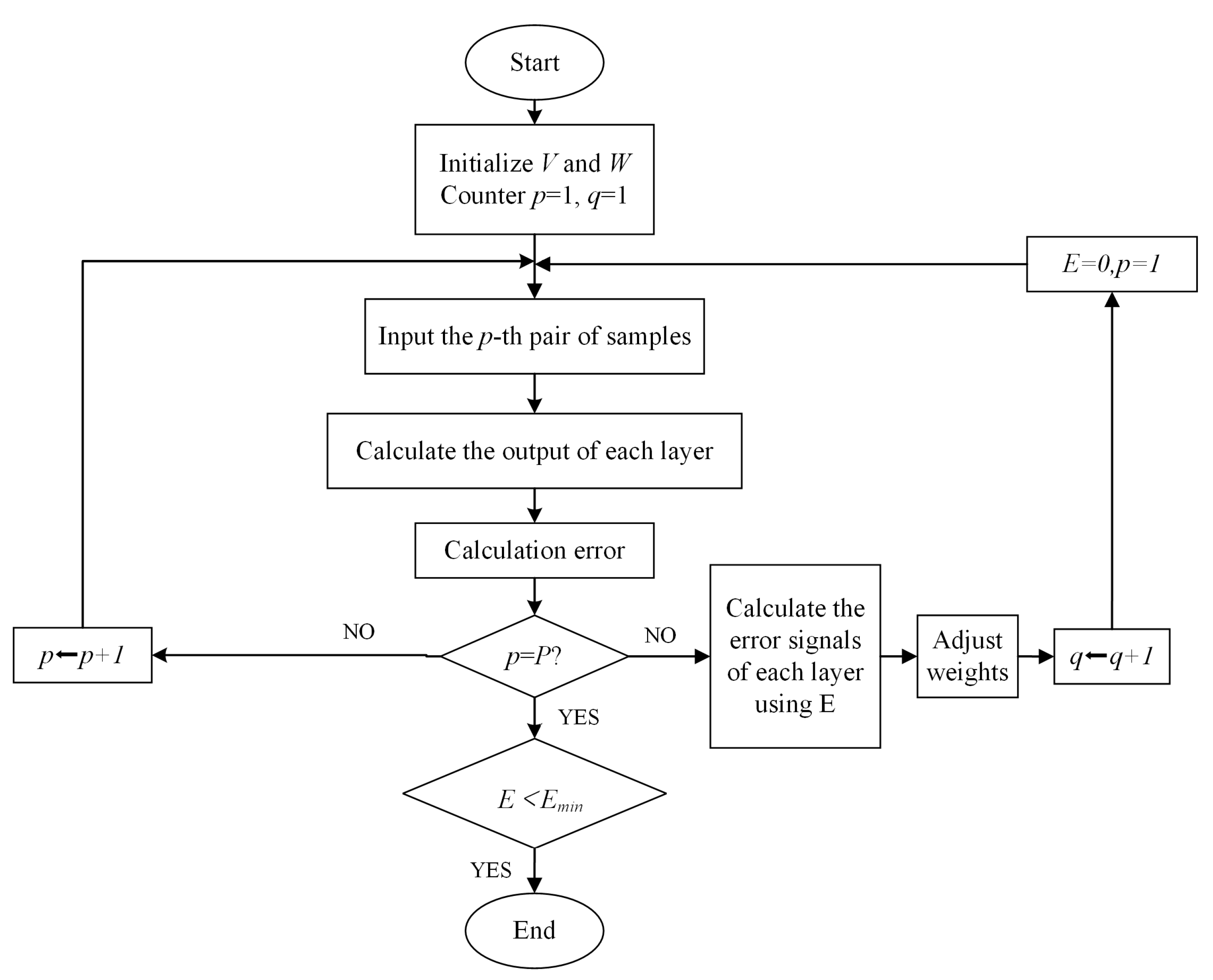
Then, based on the total error E , the error signals of each layer are calculated and the weights are adjusted. This batch processing method for accumulating errors is called batch training, also known as periodic training or batch processing. When the total error E is less than the preset error value E m i n after multiple iterations, the algorithm process is determined to be over, as shown in Figure 2.
(4) Reason for selection
Based on the general approximation theorem, a single hidden layer architecture is adopted to balance the modeling ability and computational efficiency of high-dimensional nonlinear state functions, while reducing the risk of overfitting and training complexity. By adjusting the hyperparameters of the system to determine the optimal number of hidden neurons, the best bias variance trade-off is achieved on the validation set to capture complex nonlinear mappings. The hyperbolic tangent activation function (tanh) is adopted due to its zero center output characteristic, which can promote a uniform gradient distribution and accelerate convergence [27]. Compared with Sigmoid, its enhanced gradient amplitude in key areas effectively alleviates the problem of gradient vanishing. Gradient descent optimization is achieved through carefully selected initial learning rates and triggering adaptive decay after verifying loss stability. This configuration ensures the stability of parameter updates while suppressing optimization oscillations. The dataset is randomly divided into three mutually exclusive subsets: the training set is used for weight updates; the validation set is used for hyperparameter adjustment and early stopping; and the test set is used for final performance evaluation. Training termination follows strict early stopping criteria: when the validation loss stops significantly improving over a continuous period of time, optimization stops and the model weights return to the optimal validation checkpoint to maintain generalization ability.

3. Results

To verify the effectiveness and accuracy of the proposed method, firstly, a high-dimensional nonlinear mathematical model is selected in this study to compare the prediction performance of the Kriging model and the BP neural network as a surrogate model under high-dimensional nonlinear state functions. Secondly, considering that the strength equation of state of rolling bearings as a multi-component transmission part often exhibits high-dimensional nonlinear characteristics in practical engineering problems [26], ball bearing 6016 is chosen as the research object for the strength reliability analysis and time-varying fatigue reliability analysis in this study.

3.1. Comparison of Prediction Performance of Surrogate Models

The target high-dimensional nonlinear mathematical model selected for this study is as follows:
g ( x ) = i = 1 n x i 2 + 1 i < j < k n x i x j x k + e i = 1 n x i
Among them, x = x 1 , x 2 , , x n as an n -dimensional input vector, and it can be clearly seen that the function has the following characteristics:
(a) High dimensional: dependent on n variables;
(b) Nonlinear: including quadratic terms, cubic cross terms, and exponential terms.
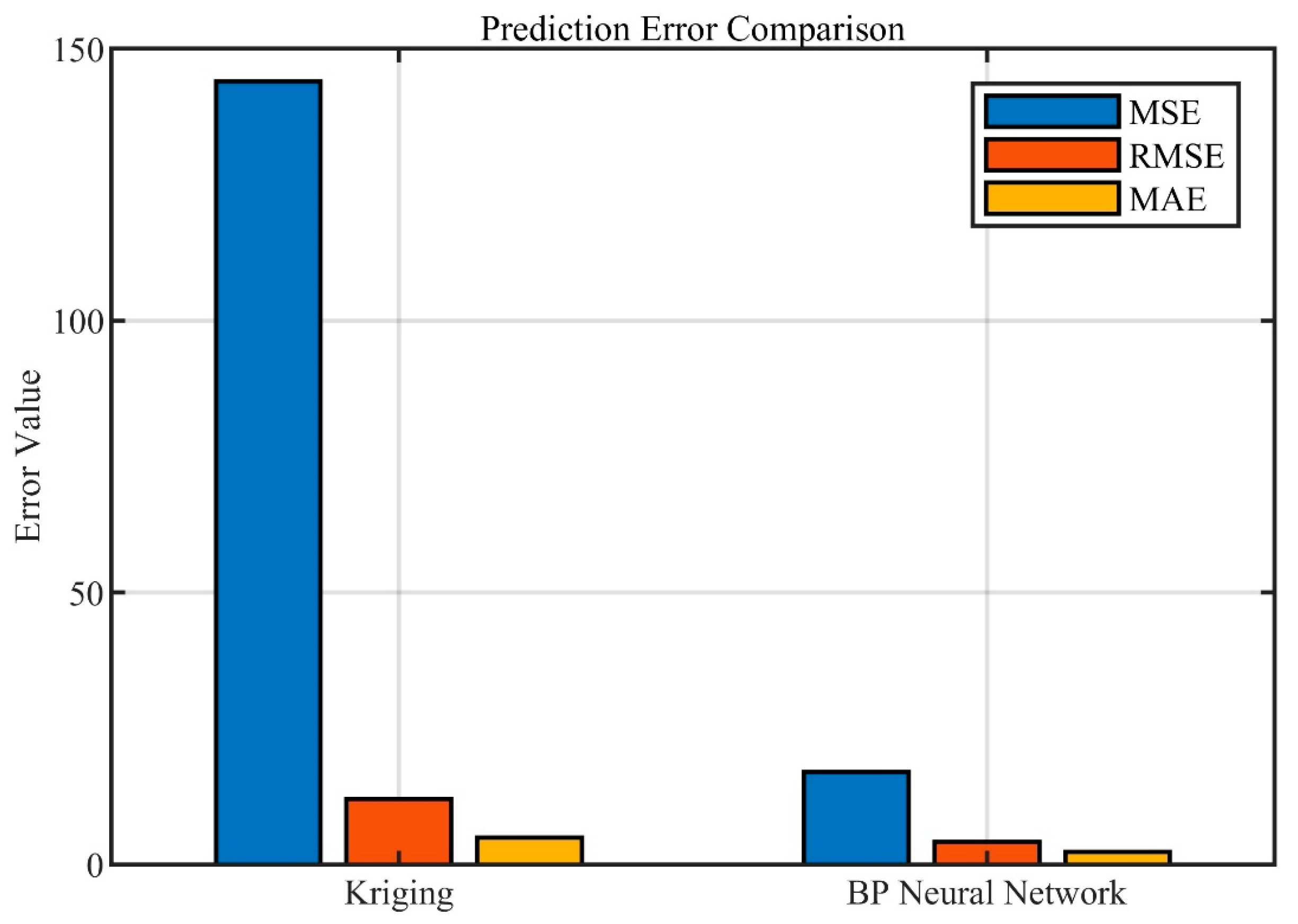
In this study, the input parameter dimension n = 10 is selected and 200 training samples and 100 test samples are randomly generated in a 10-dimensional space of [−1, 1]. In this study, the Kriging model [28] and BP neural network surrogate model were constructed based on MATLAB R2024b software using DACE toolbox and neural network toolbox, respectively. The test sample set was predicted after the model training was completed, and the mean square error (MSE), root mean square error (RMSE) and mean absolute error (MAE) were calculated based on the prediction results. The comparison results are shown in Figure 3.
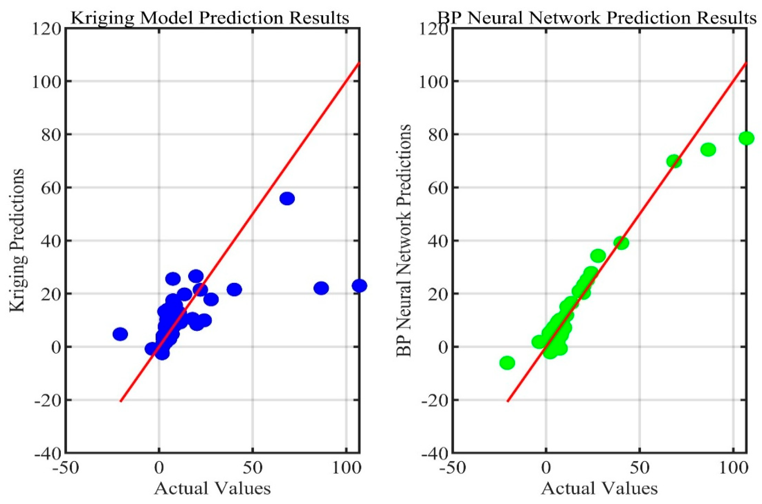
It can be seen that the surrogate model constructed by the BP neural network method has smaller prediction errors MSE, RMSE, and MAE on the test set compared to the Kriging model. Comparing the predicted values and true values of the two models on the test set as shown in Figure 4, it can be more intuitively seen that the proposed BP neural network has better prediction performance for the currently set target high-dimensional nonlinear state function.
A t-test was conducted to analyze the prediction errors between the two models, yielding a p-value of 0.0039, a t-statistic of −2.9557, and a degree of freedom of 99, with the 95% confidence interval being [−3.0963, −0.6089]. This suggests that there is a statistically significant difference in prediction performance between the two models at the 0.05 significance level, further verifying the advantage of the BP neural network in terms of prediction accuracy under the current high-dimensional nonlinear scenario.

3.2. Reliability Analysis of 6016 Bearing Strength

The size parameters, material parameters, and operating conditions of rolling ball bearings directly affect the contact stress between balls and raceways, thereby affecting the strength and reliability of bearings [12]. By studying the size, material, and operating parameters of the research object, a finite element model is established to calculate the contact stress between the balls and the raceways [29]. The failure of the rolling ball bearing is judged based on whether the contact stress exceeds the strength threshold. This process can be described by a typical high-dimensional nonlinear state equation problem. The basic parameters of the standard deep groove ball bearing 6016 used in this article are as follows: outer diameter D = 125 mm, inner diameter d = 80 mm, and ball count Z = 14. The working conditions were selected as mild: rotational speed n = 1000 r/min, radial force F r = 500 N, to prevent the failure mode of the bearing from changing due to overly extreme working conditions [29]. The material selected is the common bearing steel GCr15, with its corresponding elastic modulus E = 208 GPa, Poisson’s ratio v = 0.3, and hardness HB = 200.
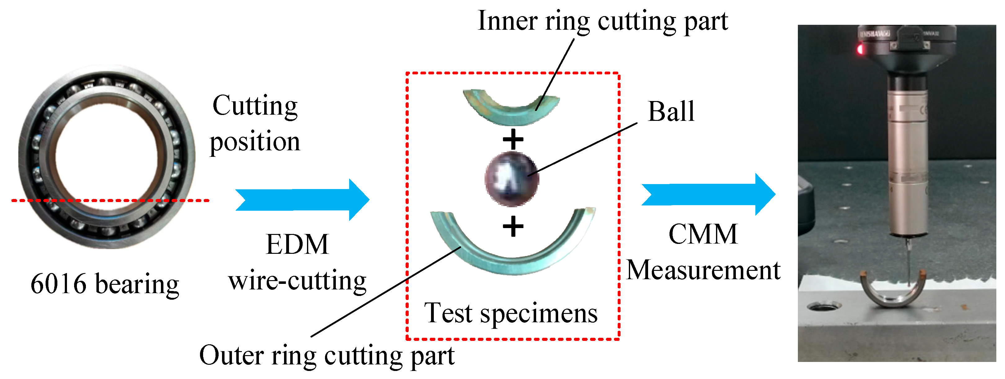
In order to illustrate the proposed method, the input vector X = D m ,   D w ,   R i ,   R o ,   n ,   F r ,   E ,   v ,   H B T of the reliability analysis algorithm of rolling bearing 6016 was constructed. Further, in order to obtain the dimensional parameters D m , D w , R i and R o in the input parameter vector X , Fifteen 6016 bearings with the same precision are chosen and processed into the measurement specimens as shown in Figure 5 by electrical discharge machining (EDM) wire-cutting and the measured values of the dimensions of the specimens were obtained by the coordinate measuring machine (CMM), respectively. Based on these 15 sets of measurements, the statistical moments of the dimensional parameters D m , D w , R i and R o in X were calculated and shown in Table 1.
Randomly generate 20 sets of input vector samples based on the data in Table 1 and solve the stress simulation by establishing a finite element model. The finite element model establishes the interactions between the inner ring and the ball, as well as between the ball and the outer ring, and assumes that all contact surfaces are smooth. All parts are constructed from GCr15 material. The outer ring is affixed with rigid constraints, connecting the inner surface of the inner ring to the central point while exerting radial concentrated force on it. Finally, the maximum contact stress under the current working condition, σ m a x X , is obtained. A BP neural network surrogate model is established between the training sample set and σ m a x X , and the proposed method is used for updating and optimization.
Assuming that the maximum allowable contact stress threshold σ ^ between the ball and the raceways is 859 MPa, the contact state function g 6016 can be defined as follows:
g 6016 = σ ^ σ m a x X ,
Clearly, when g 6016 0 , it indicates a safe state; conversely, when g 6016 < 0 , it signifies a failed state. MCS is widely recognized as the most accurate reliability calculation method under the condition of sufficient sample size (>10 × 106) [30]. The previous examples in this paper have already demonstrated the superiority of the adopted BP neural network method over the Kriging model in high-dimensional nonlinear problems. Therefore, under the same condition of constructing a surrogate model between input parameters and state functions using BP neural networks, the comparison between the MCS method and the fourth-order moment method adopted in this paper can prove the accuracy and efficiency of the proposed method in actual high-dimensional nonlinear problems. The reliability outcomes derived from the proposed BP-FM method are juxtaposed with the results from the Monte Carlo simulation utilizing the BP neural network (BP-MCS) method, as illustrated in Table 2.
10 6 The table illustrates that both methods utilize the identical BP neural network surrogate model when dealing with limited samples, resulting in minimal differences in the calculated reliability outcomes. Nevertheless, the proposed BP-FM method demonstrates a significantly reduced number of predictions for the state function compared to the BP-MCS, providing greater benefits in terms of efficiency.

3.3. Reliability Analysis of Stable Time-Varying Fatigue of 6016 Bearings

The method proposed in this article has a more significant efficiency advantage compared to the BP-MSC method when applied to time-varying reliability problems, taking into account the costs associated with cumulative reliability calculations at sequential individual time points.
On the basis of the calculation example of contact reliability of rolling bearings, considering the cumulative fatigue damage of rolling bearings under steady time-varying conditions [31,32], the 6016 bearing steady time-varying fatigue cumulative state equation g f 6016 can be constructed as follows:
g f 6016 = 1 D r b X T × t ,
where D r b X is the fatigue rate factor corresponding to one stress cycle under the current input parameter X. The specific calculation method can be based on the previous work of our research group [31], where T represents the time corresponding to one stress cycle. By using the method proposed in this article to calculate reliability and setting a time interval t = 10 h, the curve of reliability varying with time is shown in Figure 6.
Choose the interval from 2600 to 3100 h in which the reliability curve exhibits significant changes, and analyze the reliability curve derived from the approach suggested alongside the reliability curve obtained through the BP-MCS method, as illustrated in Figure 7.
It can be seen that the calculation results of the two methods are basically consistent within the interval of 2600–3100 h. Further selecting time points t = 2800 h, t = 2850 h, t = 2900 h, t = 2950 h and t = 2992 h, the proposed method for predicting the state function 1000 times was compared with the reliability calculation results of BP-MCS 106 times, as shown in Table 3.
Based on the findings presented in Table 3, it is evident that, firstly, the estimation errors between the approach introduced in this study and the BP-MCS method are relatively minor across various time points, with the highest error noted at t = 2992 h. At this instance, the reliability estimation error values computed by both methods stand at 0.4121%. Furthermore, the prediction frequency of the state function generated by the approach outlined in this research is considerably lower than that of the BP-MCS technique. This indicates that the method discussed in this paper enhances computational efficiency for reliability analyses within stationary time-varying state equations.

4. Conclusions

Based on previous research on the adaptive Kriging fourth-order moment method (AK-FM) [12], our research group discovered its weakness when dealing with high-dimensional nonlinear problems, which is consistent with the conclusions reached by other scholars in recent years in the practical application research of the adaptive Kriging Monte Carlo simulation method (AK-MCS) [33]. To address high-dimensional nonlinear problems under limited sample conditions, this paper proposes a reliability analysis method that combines a BP neural network with an improved fourth-order moment method. Quantitative validation confirms the superiority of the BP model: in predicting a 10-dimensional nonlinear function, the BP model exhibits a significantly lower RMSE than the Kriging model (t-test, p = 0.0039), demonstrating stronger fitting capability for high-dimensional nonlinearity. For the stress-strength reliability analysis of 6016 bearings, its reliability prediction result differs from that of BP-MCS by only 0.12%, while the computational efficiency is improved by 3.19 times. In the time-varying fatigue analysis of 6016 bearings, the maximum error between the proposed method and BP-MCS at critical time points is merely 0.4121%, with the proposed method requiring only 1000 predictions, which is far fewer than the 106 predictions needed for BP-MCS.
The originality lies in three aspects: (1) bridging the fourth-order moment method’s limitation in linking moments of variables and state functions via a BP surrogate model; (2) achieving higher accuracy than Kriging-based methods in high-dimensional scenarios; (3) retaining the efficiency of moment methods while adapting to limited-sample contexts.
Notably, the method has limitations: its accuracy may degrade for ultra-high-dimensional problems (n > 50) or extreme nonlinearity; and it relies on BP network training quality, risking underfitting with extremely scarce samples. It is most suitable for high-dimensional nonlinear systems (n ≤ 30) with limited data and time-varying characteristics. Of course, the method proposed in this paper is an attempt to combine the BP neural network method with the fourth-order moment method. Other advanced neural network methods also have great potential to be combined with the fourth-order moment method. In the future, how to enhance the accuracy of uncertainty quantification while maintaining the computational efficiency advantage of the fourth-order moment method will be a hot direction for the application of neural network methods in the fourth-order moment method.

Author Contributions

Conceptualization, K.Y. and S.E.; methodology, K.Y.; software, S.E.; validation, K.Y., W.L. and J.X.; formal analysis, W.L.; investigation, S.E.; resources, Y.W.; data curation, X.Y.; writing—original draft preparation, W.L.; writing—review and editing, S.E.; visualization, X.Y.; supervision, Y.W.; project administration, X.Y.; funding acquisition, K.Y. All authors have read and agreed to the published version of the manuscript.

Funding

This research was supported by the Key Research and Development Program of Heilongjiang Province (Grant No. 2022ZX07D01), the Heilongjiang Provincial Natural Science Foundation (Grant No. LH2022E038), the Fundamental Research funds for the Central Universities (Grant No. 3072025CFJ0309) and Open Project of Key Laboratory of the Ministry of Education (Grant No. B202303).

Institutional Review Board Statement

Not applicable.

Informed Consent Statement

Not applicable.

Data Availability Statement

The original contributions presented in the study are included in the article; further inquiries can be directed to the corresponding author.

Conflicts of Interest

The authors declare no conflicts of interest.

Abbreviations

The following abbreviations are used in this manuscript:
BPBack-Propagation
MCSMonte Carlo Simulation
SORMSecond-Order Reliability Method
MPPMost Probable Point
NNNeural Networks
SVMSupport Vector Machines
PCEPolynomial Chaos Expansion
ANNArtificial Neural Network
DNNsDeep Neural Networks
RBFRadial Basis Function
CNNsConvolutional Neural Networks
BP-FMBack Propagation—Fourth-order Moment
FOSMFirst-Order Second-Moment
FEMFinite Element Method
MSEMean Square Error
RMSERoot Mean Square Error
MAEMean Absolute Error
EDMElectrical Discharge Machining
CMMCoordinate Measuring Machine

Appendix A

The differential calculations related to Equations (24) and (25) are as follows.
For the output layer:
Δ w j k = E w j k = E g k g k n e t k n e t k z j z j w j k
δ k g = E n e t k = E g k g k n e t k = E g k f n e t k = d k g k g k 1 g k
For the input layer:
Δ v i j = E v i j = E g k g k n e t k n e t k z j z j n e t j n e t j v i j
δ j z = E n e t j = E g k g k n e t k n e t k z j z j n e t j
E g k = d k g k
E z i = k = 1 1 d k g k f n e t k w j k
δ j z = k = 1 l δ k g w j k z j 1 z j

References

  1. Al-Mosawe, D.; Neves, L.; Owen, J. Accelerating reliability analysis of deteriorated simply supported concrete beam with a newly developed approach: MCS, FORM and ANN. Structures 2024, 60, 105962. [Google Scholar] [CrossRef]
  2. Liu, J.; Liu, Y.; Wang, G.; Lu, N.; Cui, J.; Wang, H. Fatigue Reliability Assessment for Orthotropic Steel Decks: Considering Multicrack Coupling Effects. Metals 2024, 14, 272. [Google Scholar] [CrossRef]
  3. Song, L.; Yu, X.; Xu, B.; Pang, R.; Zhang, Z. 3D slope reliability analysis based on the intelligent response surface methodology. Bull. Eng. Geol. Environ. 2021, 80, 735–749. [Google Scholar] [CrossRef]
  4. Kumar, A.; Pandit, B.; Tiwari, G. Reliability-based stability analysis of large rock slopes with different failure mechanisms using response surface methodology. Environ. Earth Sci. 2022, 81, 51121. [Google Scholar] [CrossRef]
  5. Shao, Z.; Li, X.; Xiang, P. A new computational scheme for structural static stochastic analysis based on Karhunen-Loeve expansion and modified perturbation stochastic finite element method. Comput. Mech. 2023, 71, 917–933. [Google Scholar] [CrossRef]
  6. Huang, J.; Yang, Q.; Cao, H.; Ma, J. Structural Reliability Analysis Using Stochastic Finite Element Method Based on Krylov Subspace. Algorithms 2024, 17, 424. [Google Scholar] [CrossRef]
  7. Amalnerkar, E.; Lee, T.H.; Lim, W. Reliability analysis using bootstrap information criterion for small sample size response functions. Struct. Multidiscip. Optim. 2020, 62, 2901–2913. [Google Scholar] [CrossRef]
  8. de la Cruz, R.; Salinas, H.S.; Meza, C. Reliability Estimation for Stress-Strength Model Based on Unit-Half-Normal Distribution. Symmetry 2022, 14, 837. [Google Scholar] [CrossRef]
  9. Xie, H.; Li, J.; Liao, D. A new structural reliability analysis method under non-parameterized probability box variables. Struct. Multidiscip. Optim. 2022, 65, 32211. [Google Scholar] [CrossRef]
  10. Zhang, T. An improved high-moment method for reliability analysis. Struct. Multidiscip. Optim. 2017, 56, 1225–1232. [Google Scholar] [CrossRef]
  11. Zhao, Y.G.; Ono, T. Moment methods for structural reliability. Struct. Saf. 2001, 23, 47–75. [Google Scholar] [CrossRef]
  12. E, S.; Wang, Y.; Xie, B.; Lu, F. An Adaptive Kriging-Based Fourth-Moment Reliability Analysis Method for Engineering Structures. Appl. Sci. 2024, 14, 3247. [Google Scholar] [CrossRef]
  13. Chen, W.; Gong, C.; Wang, Z.; Frangopol, D.M. Application of first-order reliability method with orthogonal plane sampling for high-dimensional series system reliability analysis. Eng. Struct. 2023, 282, 115778. [Google Scholar] [CrossRef]
  14. Dong, M.; Cheng, Y.; Wan, L. A Novel Adaptive Bayesian Model Averaging-Based Multiple Kriging Method for Structural Reliability Analysis. Ieee Trans. Reliab. 2025, 74, 2185–2199. [Google Scholar] [CrossRef]
  15. Liu, T.; Meidani, H. Graph Neural Network Surrogate for Seismic Reliability Analysis of Highway Bridge Systems. J. Infrastruct. Syst. 2024, 30, 050240044. [Google Scholar] [CrossRef]
  16. Li, C.; Wen, J.-R.; Wan, J.; Taylan, O.; Fei, C.-W. Adaptive directed support vector machine method for the reliability evaluation of aeroengine structure. Reliab. Eng. Syst. Saf. 2024, 246, 110064. [Google Scholar] [CrossRef]
  17. Zakian, P. Stochastic finite cell method for structural mechanics. Comput. Mech. 2021, 68, 185–210. [Google Scholar] [CrossRef]
  18. Kudela, J.; Matousek, R. Recent advances and applications of surrogate models for finite element method computations: A review. Soft Comput. 2022, 26, 13709–13733. [Google Scholar] [CrossRef]
  19. Jospin, L.V.; Laga, H.; Boussaid, F.; Buntine, W.; Bennamoun, M. Hands-On Bayesian Neural Networks—A Tutorial for Deep Learning Users. IEEE Comput. Intell. Mag. 2022, 17, 29–48. [Google Scholar] [CrossRef]
  20. Fu, Z.; Xu, W.; Liu, S. Physics-informed kernel function neural networks for solving partial differential equations. Neural Netw. 2024, 172, 106098. [Google Scholar] [CrossRef]
  21. Zafar, A.; Aamir, M.; Nawi, N.M.; Arshad, A.; Riaz, S.; Alruban, A.; Dutta, A.K.; Almotairi, S. A Comparison of Pooling Methods for Convolutional Neural Networks. Appl. Sci. 2022, 12, 8643. [Google Scholar] [CrossRef]
  22. Wang, J.; Li, Y.-H.; Wang, D.; Chai, M. A reliability calculation method based on ISSA-BP neural network. Int. J. Struct. Integr. 2024, 15, 1249–1267. [Google Scholar] [CrossRef]
  23. Dong, Z.; Sheng, Z.; Zhao, Y.; Zhi, P. Robust optimization design method for structural reliability based on active-learning MPA-BP neural network. Int. J. Struct. Integr. 2023, 14, 248–266. [Google Scholar] [CrossRef]
  24. Xie, B.; Wang, Y.; Zhu, Y.; Lu, F. A novel reliability analysis method combining adaptive relevance vector machine and subset simulation for small failure probability. Struct. Multidiscip. Optim. 2023, 66, 473. [Google Scholar] [CrossRef]
  25. Zhang, T.; He, D. A Reliability-Based Robust Design Method for the Sealing of Slipper-Swash Plate Friction Pair in Hydraulic Piston Pump. IEEE Trans. Reliab. 2018, 67, 459–469. [Google Scholar] [CrossRef]
  26. Zhang, T. Matrix description of differential relations of moment functions in structural reliability sensitivity analysis. Appl. Math. Mech.-Engl. Ed. 2017, 38, 57–72. [Google Scholar] [CrossRef]
  27. Ma, L.; Tian, F. Pneumonia Incidence Rate Predictive Model of Nonlinear Time Series Based on Dynamic Learning Rate BP Neural Network. Fuzzy Inf. Eng. 2010, 1, 739–749. [Google Scholar]
  28. Xie, B.; Peng, C.; Wang, Y. Combined relevance vector machine technique and subset simulation importance sampling for structural reliability. Appl. Math. Model. 2023, 113, 129–143. [Google Scholar] [CrossRef]
  29. Xie, B.; Wang, Y.; Zhu, Y.; E, S.; Wu, Y. Vibration response-based time-variant reliability and sensitivity analysis of rolling bearings using the first-passage method. Reliab. Eng. Syst. Saf. 2025, 256, 110706. [Google Scholar] [CrossRef]
  30. Li, P.; Wang, Y. An active learning reliability analysis method using adaptive Bayesian compressive sensing and Monte Carlo simulation (ABCS-MCS). Reliab. Eng. Syst. Saf. 2022, 221, 108377. [Google Scholar] [CrossRef]
  31. E, S.; Wang, Y.; Xie, B.; Lu, F. A Reliability-Based Robust Design Optimization Method for Rolling Bearing Fatigue under Cyclic Load Spectrum. Mathematics 2023, 11, 2843. [Google Scholar] [CrossRef]
  32. Xie, B.; Wang, Y.; Zhu, Y.; Liu, P.; Wu, Y.; Lu, F. Time-variant reliability analysis of angular contact ball bearing considering the coupled effect of rolling contact fatigue damage and wear. Reliab. Eng. Syst. Saf. 2024, 241, 109667. [Google Scholar] [CrossRef]
  33. Wang, T.; Chen, Z.; Li, G.; He, J.; Shi, R.; Liu, C. Adaptive Kriging-based probabilistic subset simulation method for structural reliability problems with small failure probabilities. Structures 2024, 70, 107726. [Google Scholar] [CrossRef]
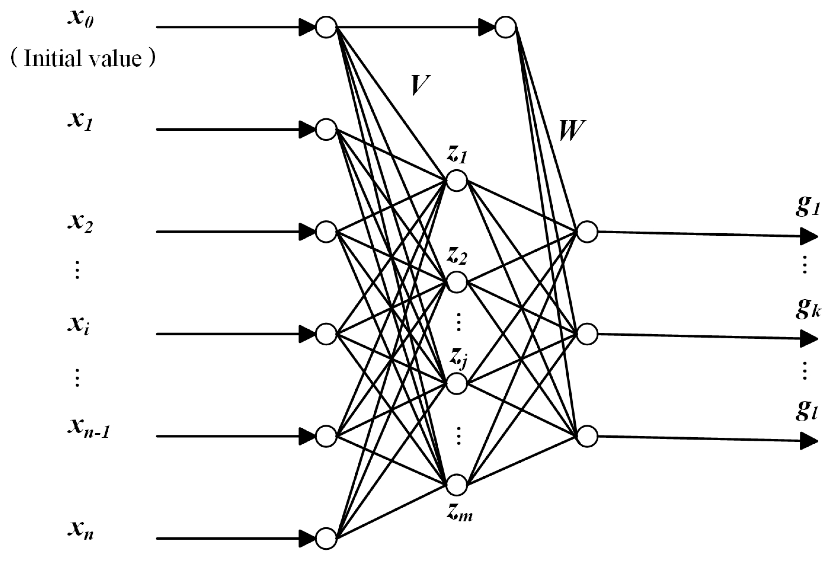
Figure 1. Schematic diagram of the constructed three-layer BP network structure.
Applsci 15 09046 g001
Figure 2. Flowchart of BP neural network algorithm for constructing state function surrogate model.
Applsci 15 09046 g002
Figure 3. Comparison of prediction errors of the Kriging model and BP neural networks for target high-dimensional nonlinear state functions.
Applsci 15 09046 g003
Figure 4. Comparison of the prediction performance of the Kriging model and BP neural networks for target high-dimensional nonlinear state functions.
Applsci 15 09046 g004
Figure 5. Processing of bearing measurement specimens (6016) and the measurement process of their dimensional parameters.
Applsci 15 09046 g005
Figure 6. Fatigue reliability curve for 6016 bearings with current parameter settings for stabilization time variation.
Applsci 15 09046 g006
Figure 7. Comparison of fatigue reliability curves of 6016 bearing at 2600–3100 h of stabilization time variation under current operating conditions.
Applsci 15 09046 g007
Table 1. Statistical parameters for the calculation of dimensional measurements of 6016 bearing test specimens.
Size ParametersMeanVariance
Center circle diameter D m (mm)102.48742.6 × 10−5
Ball diameter D w (mm)13.49403.9 × 10−6
Inner ring groove radius R i (mm)7.10101.2 × 10−6
Outer ring groove radius R o (mm)6.99601.3 × 10−6
Table 2. Comparison of contact reliability results of 6016 bearings.
MethodInitial Training Sample SizeNumber of Predictions Running Time sReliability
/%
Relative
Error/%
BP-FM2010002.6683.530.1438
BP-MCS20 10 6 8.4983.41/
Table 3. Comparison of reliability calculation results at specific time t .
Point of TimeMethodInitial Training Sample SizeNumber of Predictions for the State FunctionReliability/%Error Value
t = 2800 hBP-FM20100094.84270.1836
BP-MSC20 10 6 94.6591
t = 2850 hBP-FM20100076.0754−0.1592
BP-MSC20 10 6 76.2346
t   = 2900 hBP-FM20100043.8098−0.2703
BP-MSC20 10 6 44.0801
t = 2950 hBP-FM20100016.65480.2491
BP-MSC20 10 6 16.4057
t = 2992 hBP-FM2010005.34470.4121
BP-MSC20 10 6 4.9326
Disclaimer/Publisher’s Note: The statements, opinions and data contained in all publications are solely those of the individual author(s) and contributor(s) and not of MDPI and/or the editor(s). MDPI and/or the editor(s) disclaim responsibility for any injury to people or property resulting from any ideas, methods, instructions or products referred to in the content.