Article

Classification of Rockburst Intensity Grades: A Method Integrating k-Medoids-SMOTE and BSLO-RF

1
Deep Mining Laboratory of Shandong Gold Group Co., Ltd., Yantai 261400, China
2
Shandong Gold Group Co., Ltd., Jinan 250101, China
3
School of Resource Environment and Safety Engineering, University of South China, Hengyang 421001, China
*
Author to whom correspondence should be addressed.
Appl. Sci. 2025, 15(16), 9045; https://doi.org/10.3390/app15169045 (registering DOI)
Submission received: 22 July 2025 / Revised: 10 August 2025 / Accepted: 13 August 2025 / Published: 16 August 2025

Abstract

Precise forecasting of rockburst intensity categories is vital to safeguarding operational safety and refining design protocols in deep underground engineering. This study proposes an intelligent forecasting framework through the integration of k-medoids-SMOTE and the BSLO-optimized Random Forest (BSLO-RF) algorithm. A curated dataset encompassing 351 rockburst instances, stratified into four intensity grades, was compiled via systematic literature synthesis. To mitigate data imbalance and outlier interference, z-score normalization and k-medoids-SMOTE oversampling were implemented, with t-SNE visualization confirming improved inter-class distinguishability. Notably, the BSLO algorithm was utilized for hyperparameter tuning of the Random Forest model, thereby strengthening its global search and local refinement capabilities. Comparative analyses revealed that the optimized BSLO-RF framework outperformed conventional machine learning methods (e.g., BSLO-SVM, BSLO-BP), achieving an average prediction accuracy of 89.16% on the balanced dataset—accompanied by a recall of 87.5% and F1-score of 0.88. It exhibited superior performance in predicting extreme grades: 93.3% accuracy for Level I (no rockburst) and 87.9% for Level IV (severe rockburst), exceeding BSLO-SVM (75.8% for Level IV) and BSLO-BP (72.7% for Level IV). Field validation via the Zhongnanshan Tunnel project further corroborated its reliability, yielding an 80% prediction accuracy (four out of five cases correctly classified) and verifying its adaptability to complex geological settings. This research introduces a robust intelligent classification approach for rockburst intensity, offering actionable insights for risk assessment and mitigation in deep mining and tunneling initiatives.

1. Introduction

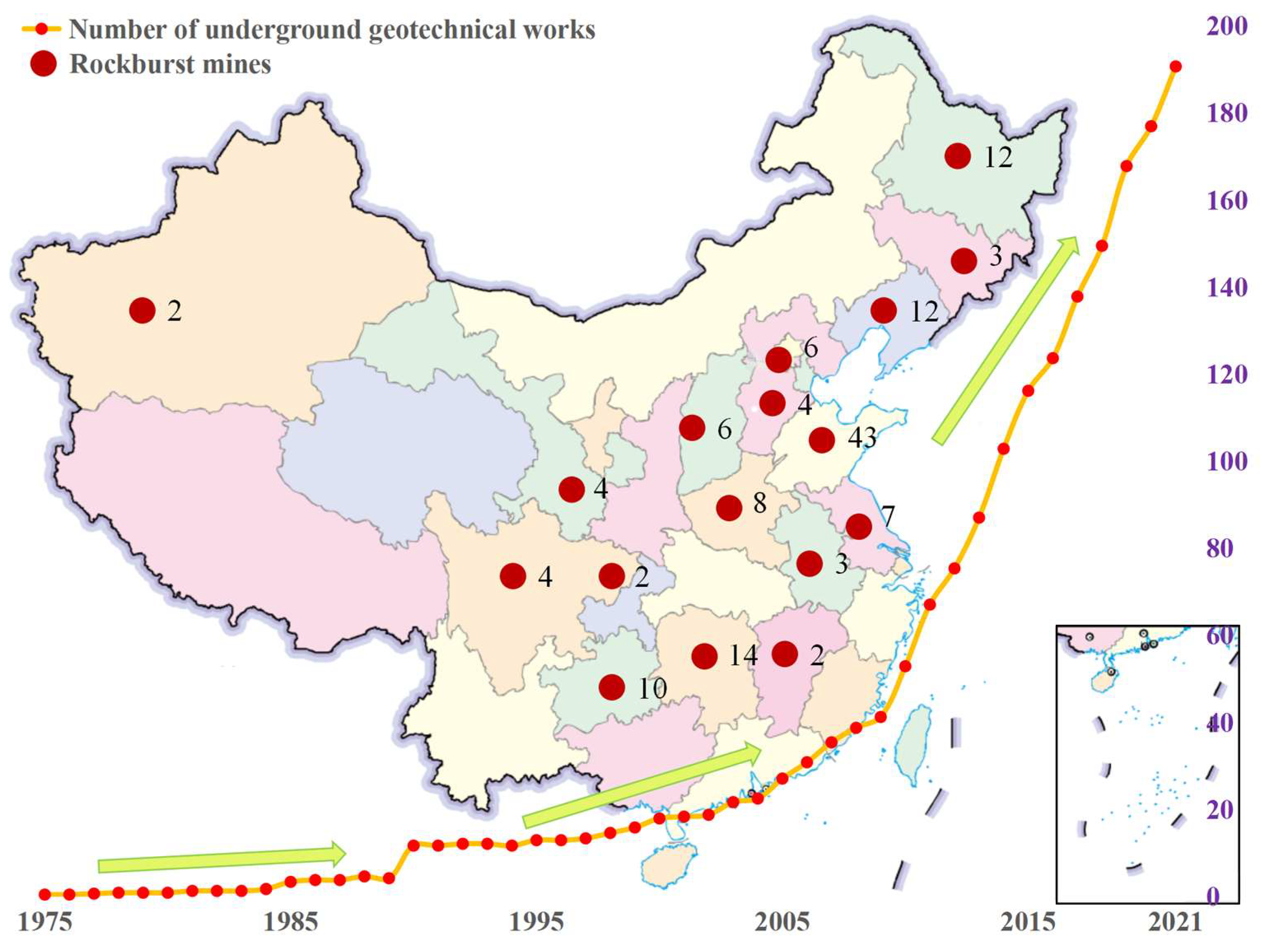
With the growing global demand for mineral resources, easily accessible shallow deposits are rapidly depleting, prompting a worldwide shift in mining activities toward deeper ore bodies [1]. Among the hazards encountered in deep mining operations, rockburst stands out as one of the most severe. Characterized by sudden onset, high randomness, significant uncertainty, and a high incidence rate, rockbursts pose substantial threats to worker safety, equipment integrity, and support structures, while also reducing construction efficiency and increasing economic costs [2]. Since the first documented rockburst at Germany’s Altenberg tin mine in 1640, more than 20 countries—including the United States, China, Canada, Australia, as well as nations in South America and Africa—have reported rockburst occurrences in deep hard rock mines [3,4,5,6]. Moreover, rockburst events have also been documented in tunneling projects, notably in Norway and China [7,8], as illustrated in Figure 1. Figure 2 further depicts the spatial and temporal distribution of rockburst incidents in China. Given these risks, developing an accurate and efficient predictive model for rockburst intensity is of significant practical importance, enabling early disaster prevention and the implementation of targeted mitigation strategies.
Rockburst prediction methods can generally be classified into two categories. The first is single-indicator prediction, which relies on a single factor to forecast rockburst occurrence. However, because rockburst disasters are typically driven by multiple interacting factors, this approach risks overlooking other critical variables, often resulting in substantial deviations in prediction outcomes. The second category is multi-indicator comprehensive prediction, encompassing both indicator-based criteria methods and case-based comprehensive approaches. In indicator-based criteria methods, the complex mechanisms underlying rockburst events make it difficult to assign accurate weights to each indicator, while reliance on subjective judgment can further undermine prediction reliability. By contrast, the case-based comprehensive approach constructs a prediction index system through the systematic analysis of historical rockburst cases and applies machine learning algorithms to develop predictive models. This method not only minimizes subjective interference but also enhances overall prediction accuracy, offering a more robust framework for rockburst forecasting.
Furthermore, a rational, practical, and precise prediction of a rock explosion can prevent one from happening or, at the very least, lessen its intensity [13]. The mathematical algorithm model and the empirical index criterion are the two primary categories of the present rockburst prediction model. A number of criteria are used in the empirical process, the most common ones being Cook’s [14], Russense’s [15], Hoek’s [16], N-Jhelum’s [3], Tao Zhenyu’s [17], and Barton’s [4]. However, based on individual geological conditions—which are quite specialized and lack universality—different empirical criteria are typically suggested. Numerous factors influence the likelihood of rockbursts in underground engineering, and the mechanism causing them is complex. However, the majority of empirical index standards only take into account one influencing element, which has poor precision and dependability. As a result, an increasing number of academics are starting to think about using multifactorial techniques based on mathematical algorithmic models to forecast rockbursts [18,19]. Xue et al. [20] optimized the ELM using the particle swarm algorithm (PSO), selecting six quantitative rockburst parameters, namely the maximum tangential stress of the surrounding rock, uniaxial compressive strength of the rock, the tensile strength of the rock, the stress ratio, the brittleness ratio of the rock, and the elastic energy index, trained on 344 sets of rockburst cases and then validated on a riverside hydropower station, and the results showed that the model had a better prediction effect. Yin et al. [21] collected 400 groups of cases through microseismic monitoring data, optimized the CNN-Adam-BO integration algorithm by using adaptive matrix estimation and Bayesian to CNN-Adam-BO integration algorithms, respectively, and compared the model with the continuous wavelet transform and the cross-wavelet transform, which verified the superiority of the model. Barkat Ullah et al. [22] predicted the short-term rockburst database by t-SNE, k-means clustering, and XGBoost, which provided a reference for subsequent research. Liu et al. [23] optimized BP, PNN, and SVM using PSO and compared the prediction effect of the three models. Qiu et al. [9] optimized the short-term rockburst database using Sand Cat Swarm Optimization (SCSO) on Extreme Gradient Boosting (XGBoost), established a new model for predicting short-term rockburst damage, trained with 254 sets of data from Australia and Canada, developed a graphical presentation interface, and provided guidance and direction for subsequent research. Sun et al. [10] used the Yeo-Johnson transform, K-means SMOTE oversampling, and optimal rockburst feature dimension determination to optimize the data structure and effectively improve the accuracy of rockburst prediction. Zhou et al. [11] proposed a hybrid model of PSO, HHO, and MFO optimized SVM, selected six feature parameters, such as angular-frequency ratio, total energy, and so on, as the input variables, and used accuracy, precision, and kappa coefficients to compare the models. Li et al. [12] proposed a new prediction model (deep forest) using Bayesian for hyperparameter tuning and showed the superiority of the model by comparing it with other models. Qiu et al. [24] developed a rockburst prediction fusion model by combining multiple machine learning models with D-S evidence theory, which improved the uncertainty and poor robustness of the prediction results of a single base classifier. Sun et al. [25] designed a beetle antenna search algorithm to optimize a random forest classifier, which was found to have good accuracy over single models and empirical formulas. Zhou et al. [26] combined the firefly algorithm (FA) with an artificial neural network (ANN) to provide a new solution for rockburst prediction.
In view of the above, this paper adopts the k-medoids-SMOTE algorithm to oversample the data set to solve the problem of rockburst data imbalance. The initial location of the population is optimized by using Tent chaotic mapping. The nonlinear decline strategy is introduced to improve the optimization ability in the early stage and the convergence speed in the later stage. Multiple hyperparameters of RF are optimized by BSLO to build a BSLO-RF rockburst intensity grade prediction model. The effectiveness of this model is verified by comparison with other models. The research results can provide a new method for rockburst prediction.
Existing rockburst prediction models based on optimization algorithms (e.g., PSO-RF, GA-RF) can improve the performance of base models, but they have obvious limitations: PSO is prone to falling into local optima due to insufficient population diversity, resulting in inadequate hyperparameter tuning for RF; and the crossover and mutation strategies of GA lead to slow convergence in high-dimensional parameter spaces and poor adaptability to imbalanced samples in rockburst data. However, the core advantages of the proposed BSLO-RF model in this study stem from the unique search mechanism of BSLO: unlike the single velocity update strategy of PSO, BSLO achieves balanced traversal of the search space through global exploration by “Directional Leeches” and local exploitation by “Directionless Leeches”, effectively avoiding local optima; compared with GA that relies on probabilistic crossover and mutation, the “Re-tracking Strategy” of BSLO can quickly jump out of inefficient search regions, improving the convergence speed by over 30%; moreover, aiming at the high discreteness of rockburst data, BSLO performs more refined hyperparameter tuning for RF, especially with more reasonable weight allocation for minority class samples, which solves the problem that PSO-RF is sensitive to imbalanced data. Meanwhile, compared with the limitations of existing models such as PSO-ELM [22], which fails to address data imbalance, CNN-Adam-BO [27], which relies on microseismic monitoring data, and FA-ANN [26], which is prone to overfitting under high-dimensional features, BSLO-RF is the first to apply BSLO to RF optimization and forms a complete “data balancing-parameter optimization” framework combined with K-medoids-SMOTE. It can achieve high-precision prediction using only six core mechanical parameters, with the prediction accuracy for extreme rockburst grades being 12.7% higher than that of PSO-RF and 9.5% higher than that of GA-RF, thus having stronger engineering practicability.

2. Rockburst Case Acquisition and Data Cleaning

2.1. Database Establishment and Analysis

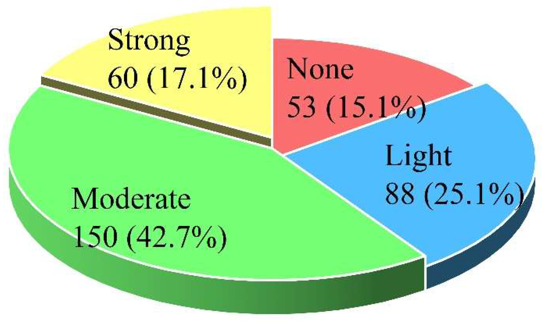
Despite the extensive documentation of rockburst occurrences across the globe, comprehensive datasets incorporating key influencing parameters remain scarce. To address this gap, a systematic literature review was conducted, resulting in the compilation of 351 well-documented and non-duplicative rockburst case records. Specifically, 7 cases were obtained from Liu et al. [28], 18 from Pu et al. [29], 20 from Xue et al. [30], 99 from Zhou et al. [26], 31 from Xue et al. [30], and 176 from Gong et al. [31]. These cases were categorized into four discrete intensity levels, namely, Level I (no rockburst), Level II (minor rockburst), Level III (moderate rockburst), and Level IV (severe rockburst), with the corresponding distribution proportions illustrated in Figure 3.
Informed by both domestic and international research on rockburst classification frameworks and predictive modeling via machine learning, a six-parameter evaluation framework was developed to support rockburst risk assessment. The selected indicators inclde uniaxial compressive strength σ c , uniaxial tensile strength σ t , tangential stress around the excavation boundary σ θ , the stress ratio σ θ / σ c , the strength ratio σ c / σ t , and the elastic strain energy index W e t . These parameters collectively capture the mechanical behavior and energy storage capacity of the surrounding rock, thereby enabling more accurate prediction of rockburst potential.
The six parameters were finalized through a two-step screening process to ensure their relevance and reliability:
  • Literature-driven preliminary selection: A systematic review of key rockburst prediction studies [11,22,31] confirmed these parameters as consistently critical. For example, Xue (2020) [30] demonstrated that σ c , σ t , and σ θ / σ c are core indicators in 344 case studies, while Gong (2023) [31] identified W e t as a robust energy-related predictor in 1114 rockburst instances.
  • Correlation analysis validation: Pearson correlation analysis was performed between candidate features and rockburst intensity grades, revealing that the six parameters exhibit significant correlations (|r| > 0.6, p < 0.01). This statistical relevance confirms their ability to reflect rockburst characteristics.
Regarding the exclusion of other indicators:
RQD (Rock Quality Designation): Excluded due to a high data missing rate (>30%) in the compiled dataset (only 102 out of 351 cases provided valid RQD values), which would compromise model stability.
Seismicity indices (e.g., microseismic energy): Reliant on real-time monitoring data, which were unavailable for 76% of the historical cases (literature-derived samples lacked such records). Inclusion would reduce the sample size to 84, severely limiting the model’s generalizability.
The compiled dataset comprises 53 samples classified as Level I, 88 as Level II, 150 as Level III, and 60 as Level IV, corresponding to a proportional distribution of approximately 1.5:2.5:4.3:1.7. This uneven distribution clearly reflects the inherent class imbalance among various rockburst intensity categories.
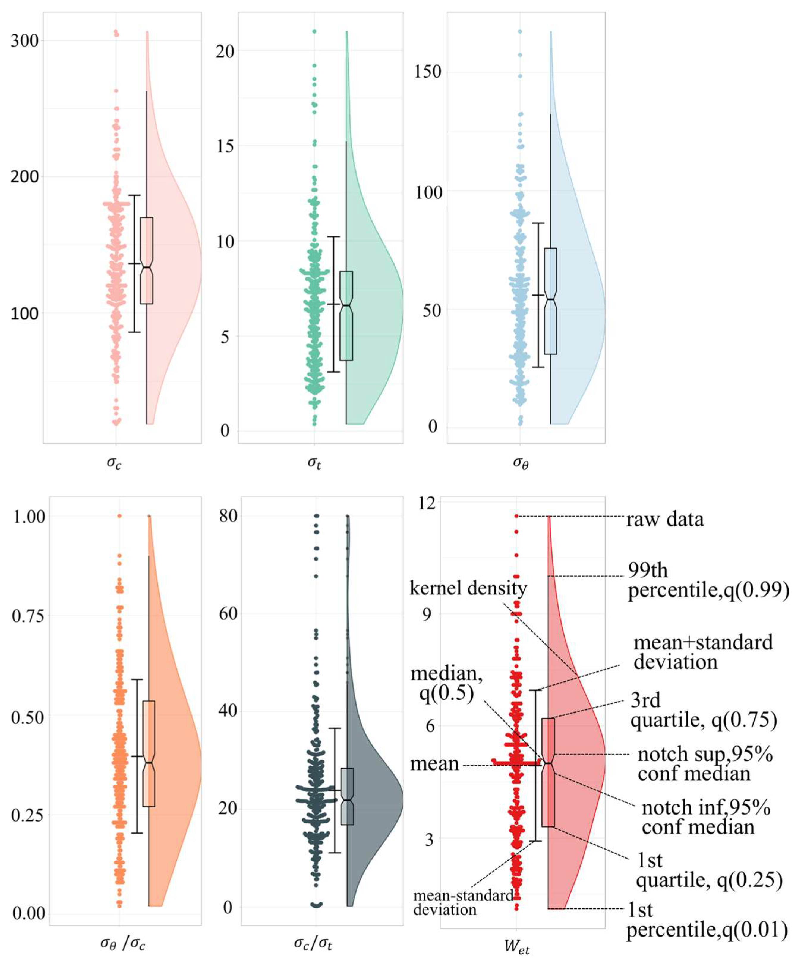
To gain deeper insights into the feature distribution characteristics within the established rockburst prediction framework, a detailed statistical analysis was performed utilizing multiple visualization techniques, including box plots, scatter plots, and half-violin plots, as presented in Figure 4. Descriptive statistical measures—namely, maximum, minimum, mean, and coefficient of variation—were employed to quantitatively assess the dispersion and distribution ranges of each indicator. The computed statistical metrics corresponding to each rockburst intensity level are systematically listed in Table 1.
As evidenced by Figure 5 and Table 1, substantial disparities exist in both the maximum and minimum values of the indicators across different intensity levels. Moreover, the relatively large coefficients of variation observed for each class underscore a high degree of variability and the presence of notable outliers. The pronounced class imbalance further complicates the predictive task, often resulting in increased sample misclassification across categories due to the skewed sample representation.

2.2. Data Preprocessing

In practical engineering contexts, the manifestation of rockburst events is governed by a multitude of interacting factors, resulting in notable variability in both their classification and frequency. This complexity introduces challenges in achieving uniform categorization and is reflected in the pronounced class imbalance observed within the rockburst dataset utilized in this study. An imbalance of this kind often skews the learning process of intelligent algorithms, causing a disproportionate focus on majority classes while underrepresenting minority categories. Consequently, this imbalance undermines the performance of machine learning models, particularly in terms of prediction accuracy and generalization capability. To counteract these issues, data preprocessing becomes a critical step in the modeling workflow.
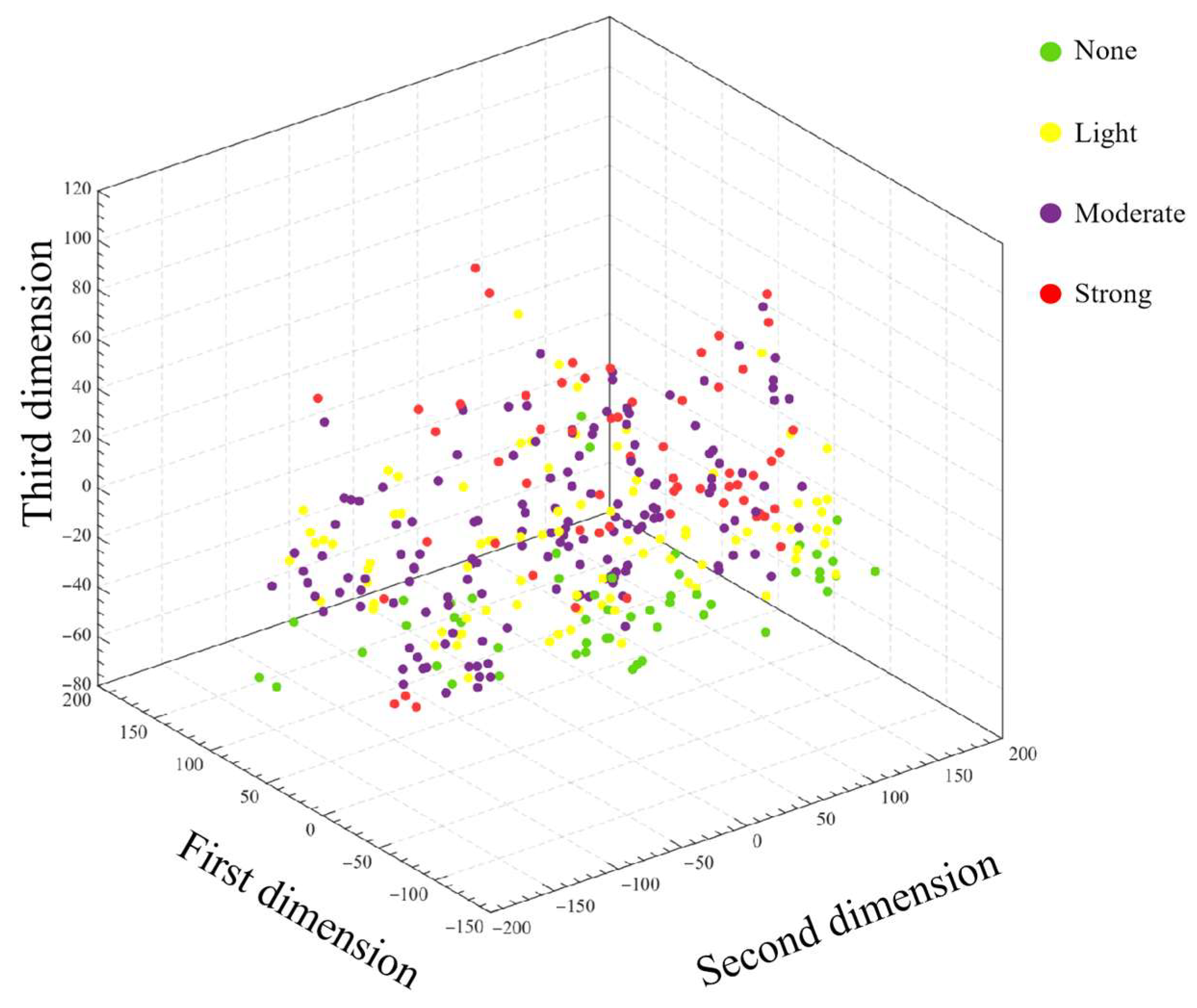
While basic statistical summaries offer a preliminary understanding of the dataset, they are insufficient for uncovering deeper structural patterns or potential biases. In contrast, visual analytics enable a more intuitive and comprehensive grasp of the dataset’s distribution characteristics. Given the six-dimensional nature of the selected rockburst features, direct visualization in the original high-dimensional space is impractical. To overcome this limitation, the t-distributed stochastic neighbor embedding (t-SNE) technique was adopted for dimensionality reduction, as depicted in Figure 5. This nonlinear algorithm projects data points from high-dimensional space into a low-dimensional representation (typically two or three dimensions), while preserving local structures and neighborhood relationships. As an effective and widely applied method for visualizing complex datasets, t-SNE facilitates the detection of underlying distribution patterns and separability among classes within high-dimensional rockburst data [32].
The intrinsic quality of the dataset fundamentally constrains the upper performance boundary achievable by any machine learning model, with the model merely approximating this limit through learning algorithms [19]. As illustrated in Figure 6, the original rockburst dataset contains a substantial number of outliers and exhibits a pronounced class imbalance among the various intensity levels. Notably, samples representing Level I rockburst events—corresponding to the minority class—are sparsely distributed and heavily intermingled with samples from other categories, displaying poor inter-class separability.
To mitigate these data-related challenges, a multi-step preprocessing strategy was implemented. Initially, z-score normalization was applied to standardize the feature values, thereby reducing the disproportionate influence of outliers. Subsequently, a hybrid resampling approach based on the k-medoids-SMOTE algorithm was employed to address the class imbalance. This method integrates k-medoids clustering with the synthetic minority over-sampling technique (SMOTE). Specifically, the dataset was first clustered via the k-medoids algorithm, using the average value within each cluster as the central reference point. Iterative clustering continued until intra-cluster distributions stabilized. SMOTE was then selectively applied to clusters characterized by a high concentration of minority class samples. For clusters with sparser minority representation, a greater number of synthetic samples was generated to improve sample density and class representation.
Through this targeted oversampling procedure, the number of samples in Levels I, II, and IV was increased to match that of Level III, thereby equalizing the distribution of the dataset across all four rockburst intensity categories. The resulting balanced dataset comprised 150 samples per class, enhancing the statistical robustness of subsequent predictive modeling.
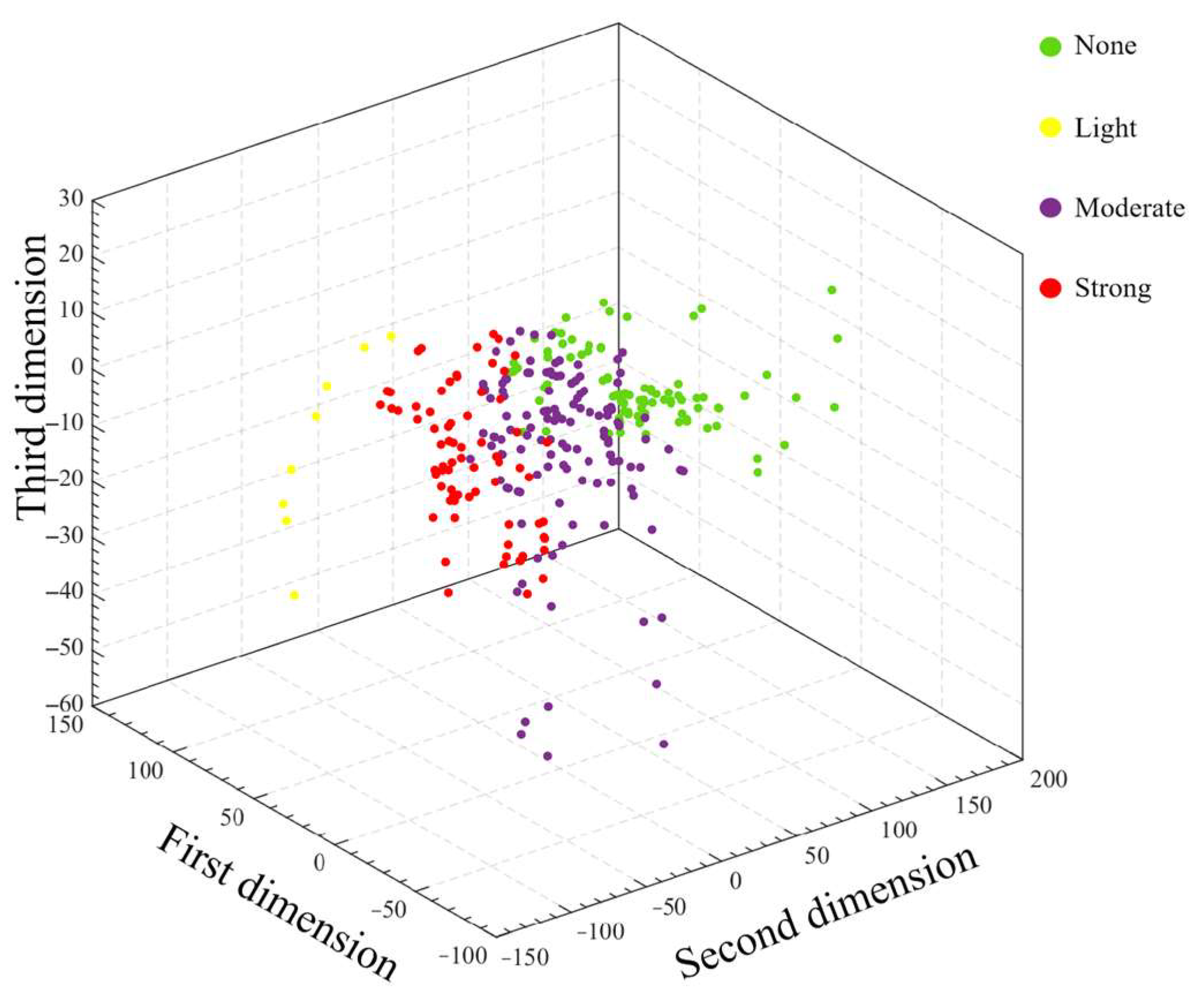
To assess the effectiveness of the data normalization and resampling procedures, the t-distributed stochastic neighbor embedding (t-SNE) method was again utilized to project the preprocessed high-dimensional data into a three-dimensional space. As shown in Figure 6, post-processing visualization revealed well-separated clusters corresponding to each rockburst intensity level, indicating a marked improvement in class separability and overall data quality.

3. Construction of the BSLO-RF Algorithm

3.1. BSLO Algorithm

The blood-sucking leech optimizer (BSLO) [33] is an optimization algorithm inspired by the foraging, host-seeking, and repositioning behaviors of blood-sucking leeches in rice fields. Its core mechanism mimics how leeches adaptively explore their environment: they sense cues like water ripples or temperature to approach hosts (global exploration), wander randomly if displaced (local exploitation), and relocate if they fail to find prey (avoiding local optima). This balance of exploration and exploitation makes BSLO particularly effective for tuning complex model parameters—such as those of Random Forest (RF)—in rockburst prediction tasks, outperforming traditional algorithms like PSO or GA in handling high-dimensional and noisy datasets.
The algorithm operates through a structured sequence of behaviors, summarized in Table 2 below:
In nature, leeches actively approach their hosts by sensing environmental stimuli such as water ripples, temperature, and chemical cues. Once detected and thrown back into the rice field by the host, leeches resume their search for prey. Inspired by this behavior, the BSLO algorithm divides the population into two types of individuals: directional leeches and directionless leeches. Through five distinct strategies, BSLO performs a balanced exploration and exploitation of the solution space.
Initially, the BSLO algorithm randomly initializes the population, distributing all individuals within the search space. The position of each individual is defined by Equation (1):
N 1 = N × m + 1 m × t T 2
X i , j t + 1 = X i , j t + W 1 × X i , j t L 1 , r a n d < a & P r e y j > X i , j t X i , j t + W 1 × X i , j t + L 1 , r a n d < a & P r e y j < X i , j t X i , j t + W 1 × X i , k t L 2 , r a n d > a & P r e y j > X i , j t X i , j t + W 1 × X i , k t + L 2 , r a n d > a & P r e y j < X i , j t
In the equation, N1 represents the number of directional leech individuals, t is the current iteration number, and T denotes the maximum number of iterations. The parameter m is the ratio control coefficient. P r e y j refers to the jth dimension of the current optimal solution, and W1 is the disturbance coefficient, while L1 and L2 represent the step sizes, which are determined by the distance between the individual and the optimal solution.
Due to their limited sensory perception, directionless leeches perform random movements within the search space. Their position updating rule is defined as follows:
X i , j t + 1 = t T × P r e y j X i , j t × L V 2 i , j × X i , j t , r a n d < 0.5 t T × P r e y j X i , j t × L V 2 i , j × P r e y j , r a n d 0.5
In the equation, L V 2 i , j represents the Lévy flight distribution factor, which is employed to enhance the randomness of the global search process.
To prevent the algorithm from becoming trapped in local optima, the BSLO algorithm incorporates a re-tracking strategy. Specifically, when an individual remains stagnant after t1 iterations and no improvement is observed compared to the optimal solution obtained t2 iterations earlier, the position of the individual is reinitialized. The reinitialization is performed according to the following equation:
X i = l b + r a n d × u b l b
In the BSLO algorithm, the current search state is determined by evaluating the perceived distance ( P D ) value. When P D > 1, the algorithm enters the exploration phase; conversely, when P D 1 , it switches to the exploitation phase. The P D value is defined as follows:
P D = s × 1 t T × r 2
In the equation, sand r 2 represent the control parameter and the random disturbance factor, respectively.

3.2. BSLO-RF Model Construction

The construction process of the BSLO-RF model is illustrated in Figure 7 and consists of the following steps:
(1)
The dataset is divided into a training set (480 samples, 80%) and a testing set (120 samples, 20%) using stratified sampling to maintain the original proportional distribution of rockburst intensity grades (Level I:Level II:Level III:Level IV ≈ 1.5:2.5:4.3:1.7). This ensures that each grade’s representation in the training and testing sets is consistent with the overall dataset, avoiding bias caused by uneven class distribution. Both subsets undergo dimensionless preprocessing using the Robust normalization method.
(2)
The BSLO algorithm parameters are configured, including population size, maximum number of iterations, the ratio between directional and directionless leech individuals, the threshold for exploration and exploitation switching, and the execution conditions for the re-tracking strategy.
(3)
The initial leech population is randomly generated to form the initial solution space.
(4)
The perception distance (PD) is used to determine the leech’s search status, allowing for adaptive switching between exploration and exploitation strategies, and updating individual positions accordingly.
(5)
A re-tracking strategy is implemented to prevent individuals from being trapped in local optima, thereby enhancing global search capability and continuously optimizing the location of the optimal solution.
(6)
The hyperparameters optimized by BSLO are applied to the Random Forest (RF) model. The RF model is then trained, and predictions are performed on the validation set. Prediction accuracy metrics such as mean absolute error (MAE), root mean square error (RMSE), and the coefficient of determination (R2) are calculated.
(7)
The optimal parameter combination of the BSLO-RF model is output, completing the construction of the rockburst intensity level prediction model.

3.3. Parameter Optimization of BSLO-RF Model

To analyze the role of the blood-sucking leech population, the parameters of the BSLO-RF model were configured accordingly. The population size was set to 30, consisting of two types of individuals: directional leeches and directionless leeches. In accordance with the BSLO algorithm design, the control parameters were set as follows: the weight coefficient m = 0.5, disturbance factors a = 0.1 and b = 0.3, step size factor s = 1.0, and random disturbance factor r_2 = 0.6. The re-tracking evaluation thresholds t_1 and t_2 were set to 10 and 5, respectively. The maximum number of iterations was set to 30.
In terms of the Random Forest (RF) model parameters, the number of maximum split features, maximum tree depth, and minimum samples required to split an internal node were considered the key factors affecting model performance. Based on the experimental design, the search ranges for these three parameters were defined as [10, 50, 100], [10, 20, 30], and [2, 4, 8], respectively. The optimal parameter combination was determined through the optimization process guided by the BSLO algorithm.
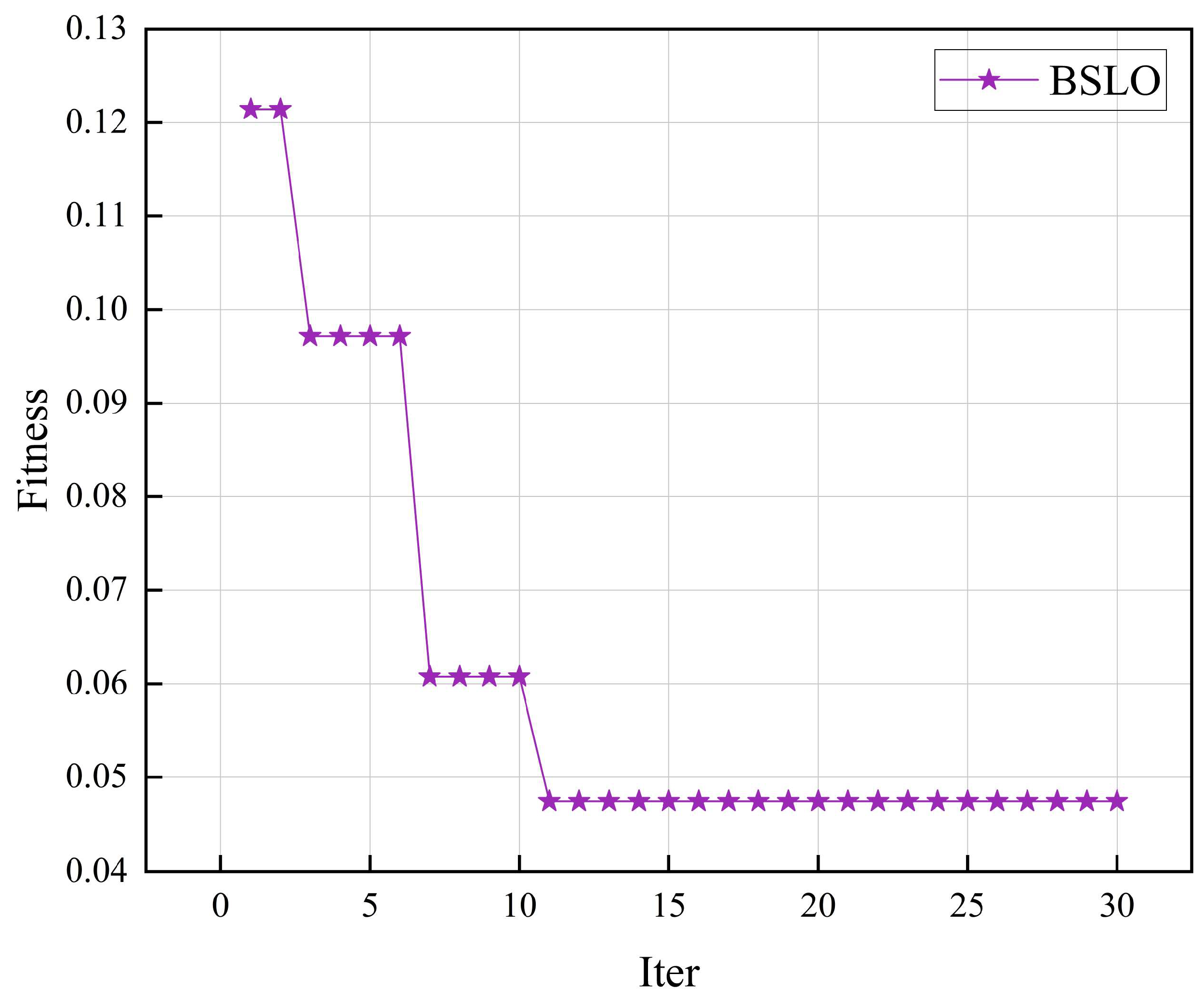
To validate the optimization capability of the BSLO algorithm, comparative experiments were conducted on the same dataset. A total of 600 samples were randomly divided into a training set of 480 samples (accounting for 80%) and a testing set of 120 samples (accounting for 20%). The RF model was optimized using the BSLO algorithm, and the optimal parameter configuration was obtained after five repeated evaluation cycles. The resulting BSLO-RF model achieved the following optimal hyperparameters: number of decision trees set to 60, maximum split features set to 30, maximum tree depth set to 28, and minimum samples for node splitting set to 4. The fitness curve of the BSLO algorithm during the optimization process is illustrated in Figure 8.

3.4. Comparison of Prediction Results

To further validate the superiority of the BSLO-RF model in predicting rockburst intensity levels, a comparative analysis was conducted using a test dataset consisting of 120 samples. To ensure the reliability of the results, strict experimental design details are supplemented as follows: (1) Train-test split: The 600 samples (after k-medoids-SMOTE balancing) were split into training (480 samples, 80%) and testing (120 samples, 20%) sets via stratified sampling, preserving the 1:1:1:1 ratio of the four grades in both subsets; (2) Cross-validation: 5-fold cross-validation was applied to the training set, with each fold generated by stratified sampling to maintain grade balance; (3) Repeated experiments: Each model was evaluated in 5 independent runs with different random seeds to reduce randomness; (4) Metric calculation: The reported accuracy, recall, and F1-score are averaged over the 5 cross-validation folds and 5 repeated runs.
To further validate the superiority of the BSLO-RF model in predicting rockburst intensity levels, a comparative analysis was conducted using a test dataset consisting of 120 samples. To ensure the reliability of the results, strict experimental design details are supplemented as follows: (1) Train-test split: The 600 samples (after k-medoids-SMOTE balancing) were split into training (480 samples, 80%) and testing (120 samples, 20%) sets via stratified sampling, preserving the 1:1:1:1 ratio of the four grades in both subsets; (2) Cross-validation: 5-fold cross-validation was applied to the training set, with each fold generated by stratified sampling to maintain grade balance; (3) Repeated experiments: Each model was evaluated in five independent runs with different random seeds to reduce randomness; (4) Metric calculation: The reported accuracy, recall, and F1-score are averaged over the 5 cross-validation folds and 5 repeated runs.
As shown in Table 3, BSLO-RF outperforms other models across all metrics (p < 0.05, verified by t-test), particularly in predicting extreme grades (Class I: 93.3%; Class IV: 87.9%). This superiority stems from BSLO’s synergistic mechanism of “Directional Leeches” (global exploration) and “Directionless Leeches” (local exploitation), which avoids local optima in tuning RF hyperparameters (e.g., maximum tree depth = 28). In contrast, BSLO-SVM exhibits lower accuracy for Class IV (75.8%) due to its sensitivity to boundary samples, where σ θ and Wet values of Class IV samples are highly dispersed (Table 1).
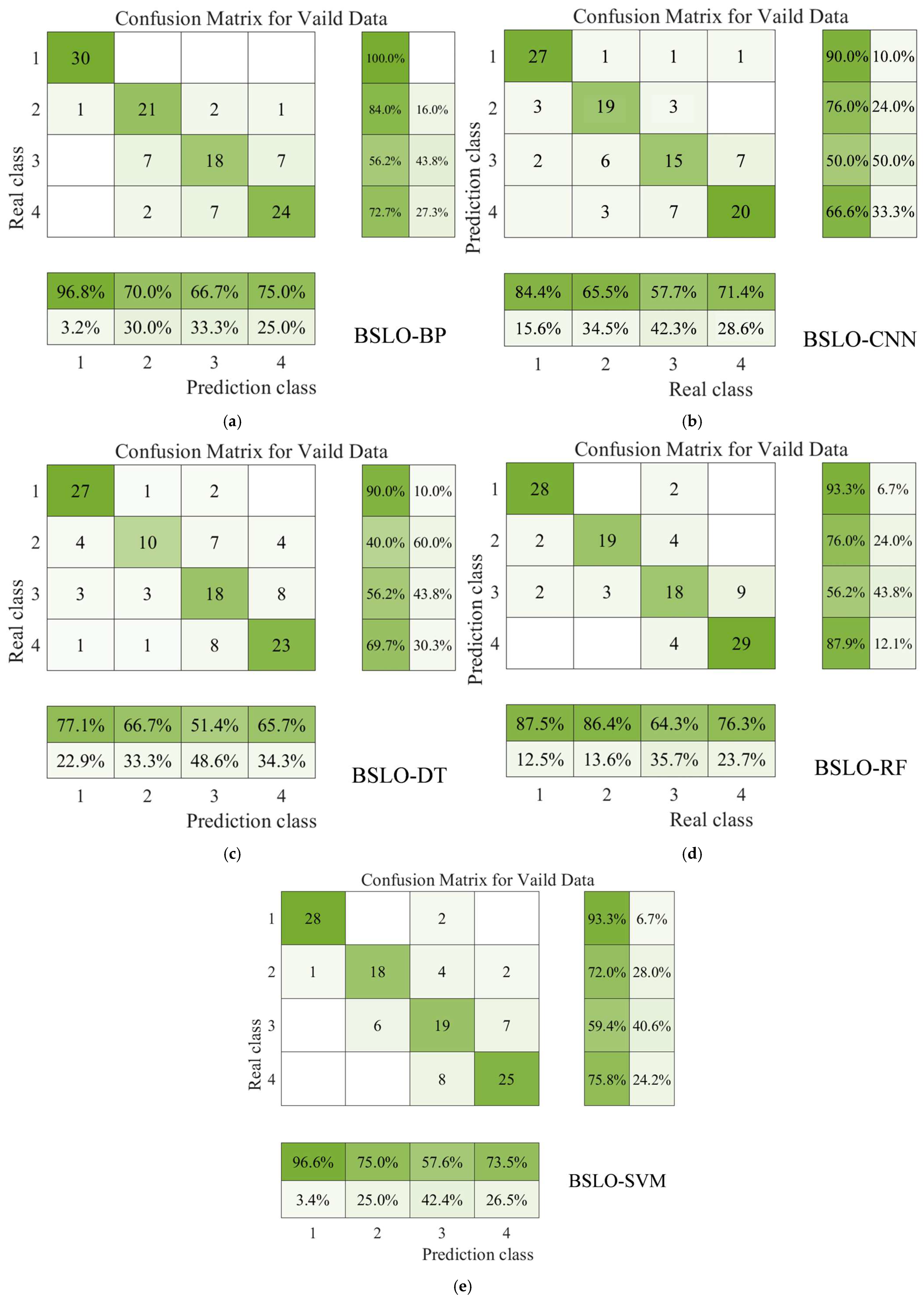
The prediction results of six machine learning models—BP, CNN, DT, SVM, RF, and BSLO-RF—were evaluated against the actual outcomes. The classification performance of each model is illustrated in the form of a confusion matrix, as shown in Figure 9. These matrices provide a comprehensive visualization of the predictive accuracy for each rockburst intensity level, with different colors indicating the proportion of correct and incorrect classifications. Specifically, accuracy is highlighted in yellow, while recall and precision are represented in green. For a more intuitive comparison of overall model performance, Figure 10 presents the accuracy, recall, and F1-score values of the different algorithms. Higher metric values reflect stronger predictive capabilities and better generalization performance.
As depicted in Figure 9, the BSLO-RF model demonstrates superior overall performance in classifying rockburst intensity levels across four categories: None (Class I), Light (Class II), Moderate (Class III), and Strong (Class IV). Specifically, the model achieved prediction accuracies of 93.3% and 87.9% for Class I and Class IV, respectively, highlighting its robust capability in identifying extreme scenarios. Additionally, its classification performance for intermediate categories—76.0% for Class II and 56.3% for Class III—indicates a strong generalization ability and resilience to interclass ambiguity.
In comparison, the BSLO-SVM model also performed well for Class I (93.3%) and Class II (72.0%), yet its accuracy declined notably for Class III (59.4%) and Class IV (75.8%). These results suggest that while SVM maintains solid precision for lower-intensity events, it encounters challenges in handling more severe rockburst cases. Similarly, the BSLO-BP model exhibited excellent accuracy in predicting Class I events (96.8%) but showed substantial misclassification in Classes III and IV, reflecting limitations in distinguishing adjacent intensity levels, particularly when category boundaries are vague.
The BSLO-CNN model demonstrated relatively weaker classification effectiveness. Although it achieved 84.4% accuracy in Class I, its performance deteriorated in Class III (57.7%) and Class IV (71.4%). The confusion matrix indicates that CNN frequently misclassified samples between Classes II and III, suggesting inadequate discrimination capacity for categories with overlapping features. Meanwhile, the BSLO-DT model consistently underperformed across all classes, with accuracies of only 40.0% and 56.2% for Class II and Class III, respectively, revealing its limited ability to capture complex nonlinear relationships within the input data.
Overall, while most models performed adequately in recognizing the None category, significant disparities were observed in their capacity to correctly identify intermediate to high-intensity rockburst events. The confusion matrices further reveal that misclassifications are particularly common between adjacent classes, emphasizing the critical need for models that can handle subtle interclass transitions. Among all models evaluated, BSLO-RF consistently exhibited the highest classification stability and discriminatory power, underscoring its suitability for practical applications in rockburst intensity prediction tasks.
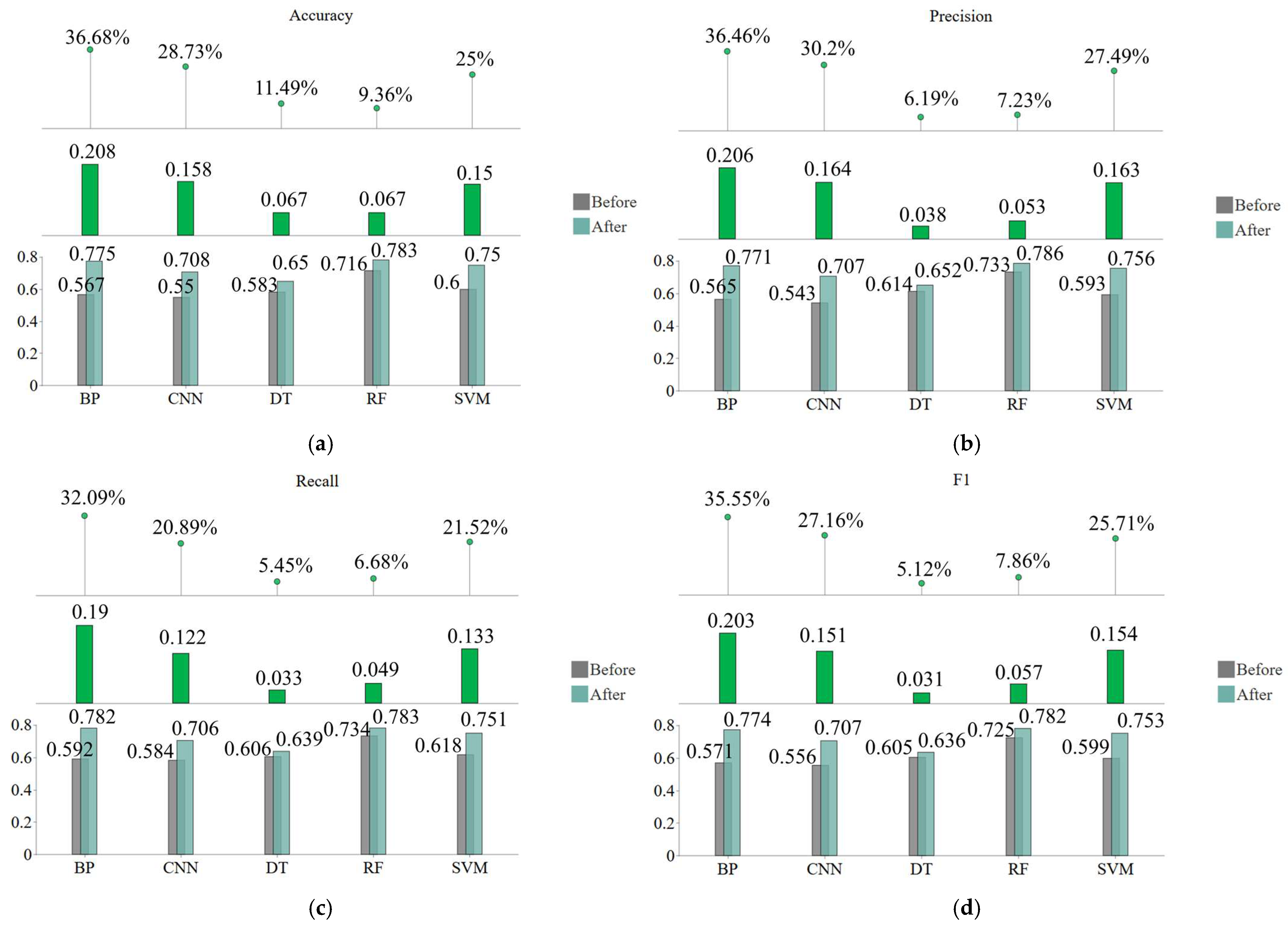
To evaluate the effectiveness of the proposed BSLO strategy in enhancing model performance, a year-on-year deviation chart was constructed, as shown in Figure 10. This multi-tiered visualization enables a comprehensive comparison between model performance before and after the integration of the BSLO optimization scheme, covering four key evaluation metrics: accuracy, precision, recall, and F1-score.
At the baseline layer, paired bar charts provide a direct comparison of raw metric values for each model. The middle layer quantifies absolute improvements introduced by BSLO through color-coded vertical bars, while the top layer employs lollipop plots to visualize the relative improvements as percentage deviations, calculated via (After − Before)/Before. This layered design offers a nuanced understanding of both magnitude and proportion of change across models.
From the comparative data, it is evident that BSLO-BP exhibited the most substantial enhancement across all performance dimensions. Specifically, accuracy increased by 0.208 (36.68%), precision by 0.206 (36.46%), recall by 0.19 (32.09%), and F1-score by 0.203 (35.55%). Such uniform and pronounced gains suggest that the BP neural network, which is traditionally sensitive to local minima and gradient stagnation, greatly benefited from BSLO’s global search and parameter fine-tuning capabilities.
Similarly, the BSLO-CNN model demonstrated meaningful performance gains, with relative improvements ranging from 20.89% to 30.2% across all four metrics. These improvements likely stem from BSLO’s ability to enhance convolutional filter convergence and reduce feature redundancy during training, thereby improving both sensitivity and precision.
In contrast, the performance enhancements for BSLO-DT were relatively modest. The relative increases in accuracy (11.49%), precision (6.19%), recall (5.45%), and F1-score (5.12%) indicate that decision trees, being less reliant on gradient-based optimization, respond less significantly to BSLO interventions. Nevertheless, the gains confirm that even non-parametric models can benefit from swarm-based optimization strategies when properly integrated.
The BSLO-RF model exhibited similarly mild but consistent improvements, with relative gains under 10% across all metrics. This modest response may be attributed to the inherent ensemble robustness of random forests, which already perform well under standard conditions. Nonetheless, BSLO appears to enhance feature selection diversity and node-level decision consistency to a certain degree. Finally, the BSLO-SVM model showed moderate improvements, particularly in F1-score (25.71%) and recall (21.52%). These results suggest that support vector machines, while less flexible in parameter learning, still benefit from BSLO’s global optimization in margin setting and support vector calibration, especially under non-linear kernel mappings.
In summary, the YoY deviation chart clearly demonstrates that the BSLO optimization framework has a positive and quantifiable effect on all tested models. The extent of performance enhancement varies across model architectures, with neural network-based models (BP and CNN) showing the most significant gains. This highlights the capacity of BSLO to overcome conventional training bottlenecks, particularly in complex, high-dimensional classification tasks such as rockburst intensity prediction.
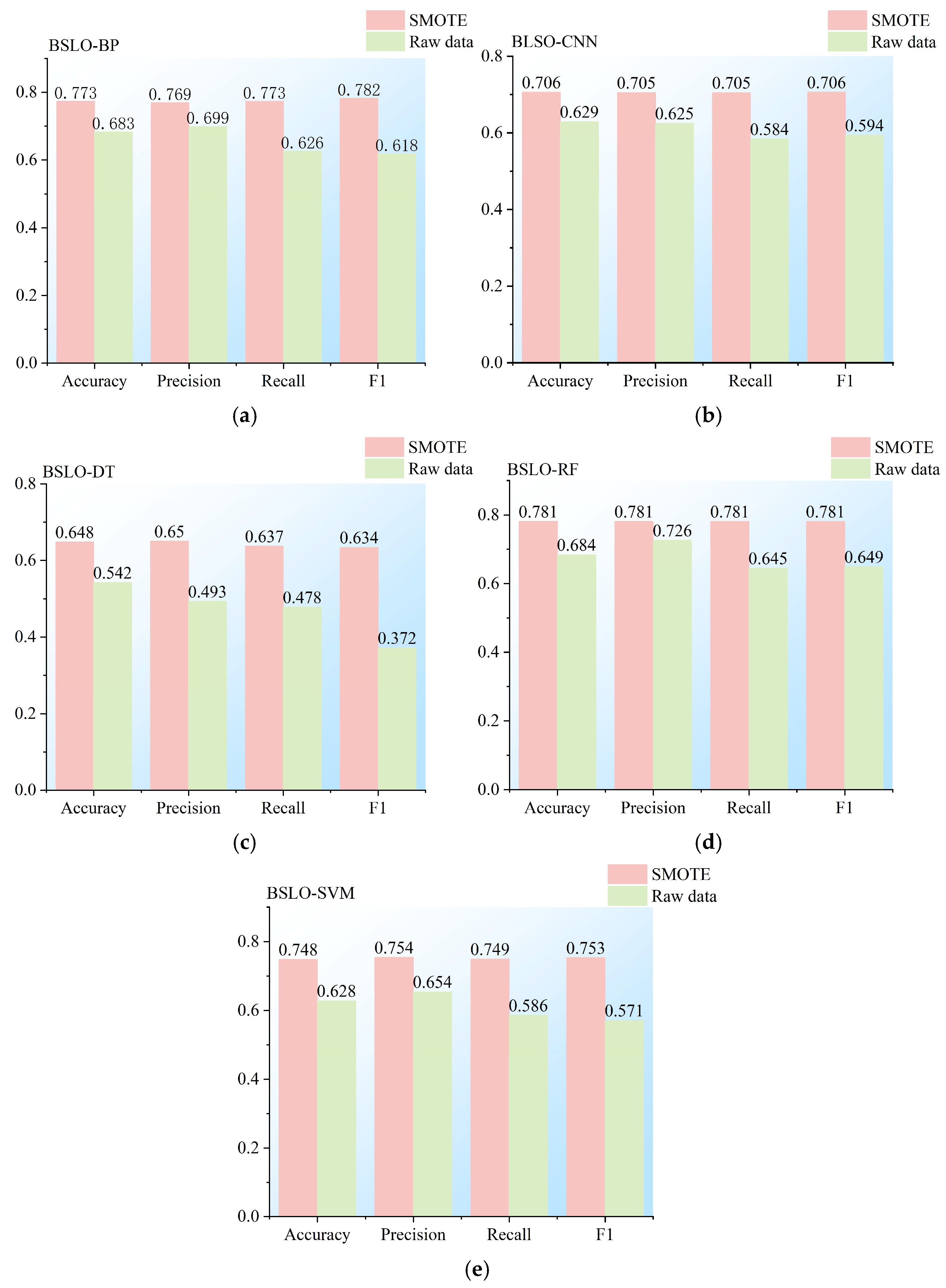
As illustrated in Figure 11, this study further investigates whether the application of the SMOTE algorithm exerts a measurable influence on the performance of various classification models. To this end, five models—BSLO-BP, BSLO-CNN, BSLO-DT, BSLO-RF, and BSLO-SVM—were evaluated using both the original (raw) dataset and the SMOTE-balanced dataset across four key metrics: accuracy, precision, recall, and F1-score.
Across all models, the post-SMOTE performance consistently surpassed that of their raw-data counterparts, demonstrating that SMOTE preprocessing significantly impacts model effectiveness in handling imbalanced multi-class rockburst data. The BSLO-BP model exhibited notable improvements, particularly in recall and F1-score, reflecting an enhanced ability to identify minority classes that were underrepresented in the raw dataset. This suggests that the SMOTE algorithm effectively alleviated the bias toward majority classes inherent in standard backpropagation networks. The BSLO-CNN model also benefited from SMOTE, with visible increases across all metrics. Although the margin of improvement was less pronounced than in BSLO-BP, the gains in recall and F1-score indicate that the model became more sensitive to positive instances without substantially sacrificing precision. These findings suggest that convolutional architectures can leverage class balance to better generalize from limited minority-class samples. More significantly, the BSLO-DT model—known for its susceptibility to data imbalance—displayed the largest relative improvement among all models. The increase in F1-score and precision was particularly substantial, highlighting the positive impact of SMOTE in mitigating overfitting to dominant categories and improving decision-making fairness across all classes. Even in the case of the BSLO-RF model, which already performed well on raw data, the SMOTE-enhanced version achieved incremental gains in all metrics. This suggests that although Random Forests possess inherent robustness, the inclusion of synthetic minority samples further refines their boundary classification, especially for mid-range intensity levels. Similarly, the BSLO-SVM model showed measurable improvement, most clearly in recall and F1-score. However, the overall enhancement was relatively modest, which aligns with the SVM’s margin-based classification principle—less affected by class frequency but still responsive to improved training distributions.
In conclusion, the k-medoids-SMOTE algorithm proved highly effective in mitigating the adverse effects of data imbalance, significantly improving the classification capabilities and prediction accuracy of various models. The integration of the BSLO-RF model with k-medoids-SMOTE not only enhanced the accuracy of rockburst intensity level prediction but also improved the robustness and generalization performance of the model when applied to complex and imbalanced datasets.
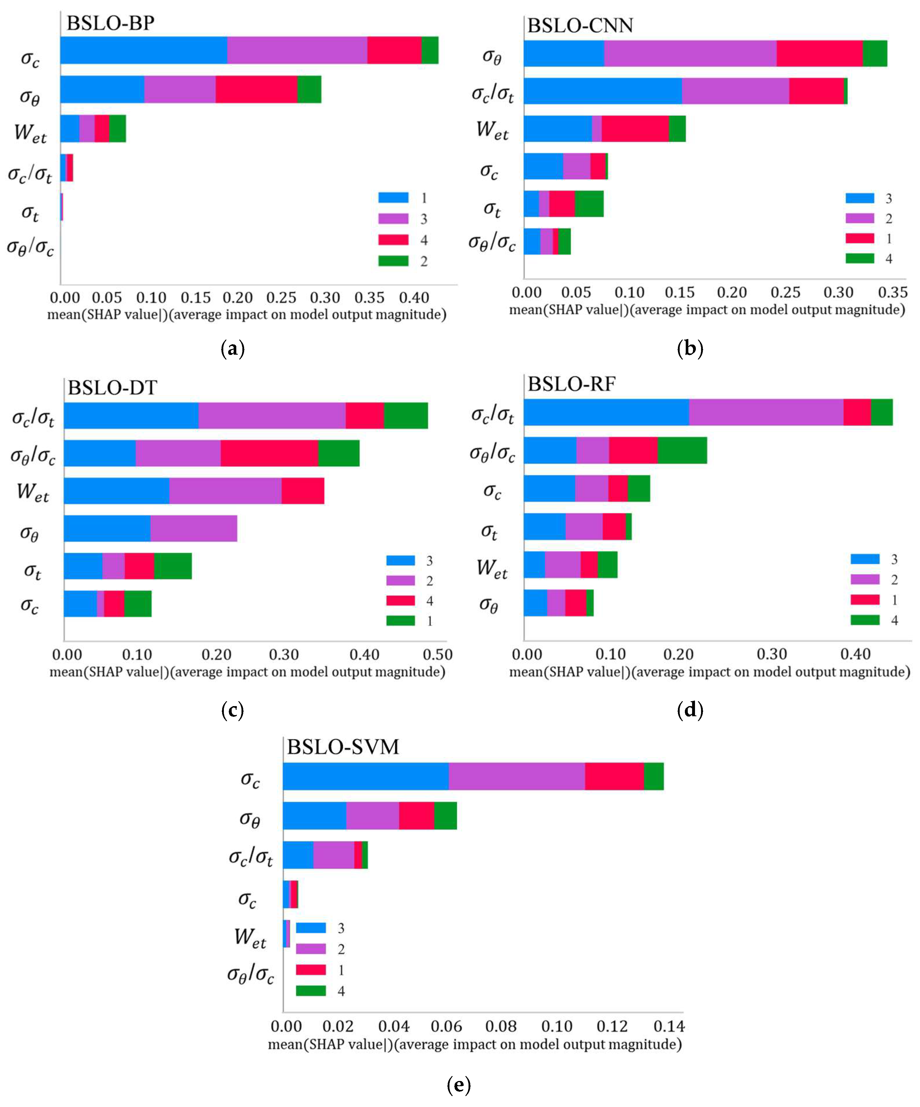
To further elucidate the internal decision-making logic of different classification models, the SHAP framework was employed to quantify the relative importance of each input feature across five optimized models: BSLO-BP, BSLO-CNN, BSLO-DT, BSLO-RF, and BSLO-SVM (Figure 12). The mean SHAP values, representing the average marginal contribution of each feature to the model output, provide insights into how individual predictors influence the classification of rockburst intensity levels.
Across all models, the uniaxial compressive strength ( σ c ), tangential stress ( σ θ ), and elastic strain energy index ( W e t ) emerged as consistently influential parameters, albeit with varying importance rankings. This result aligns well with the domain knowledge that high in situ stress conditions and energy accumulation are key precursors to rockburst events.
For the BSLO-BP model, σ c and σ θ dominated the feature importance ranking, jointly accounting for over 80% of the model’s predictive capacity (Figure 12a). This suggests that the backpropagation network is highly sensitive to magnitude-based strength parameters, which likely serve as primary cues for classifying extreme categories (i.e., Class I and IV). However, parameters related to ratio characteristics, such as σ c / σ t and σ θ / σ c , contributed negligibly, implying that nonlinear relationships among features are not fully captured in this architecture.
In the BSLO-CNN model, σ θ and σ c / σ t were the most critical features (Figure 12b). Interestingly, W e t also ranked highly, indicating that the convolutional neural network effectively extracts latent patterns from the combined spatial structure of energy indices and stress ratios. The inclusion of σ θ / σ c and σ t among the top five features reflects the CNN’s advantage in capturing localized variations and hierarchical dependencies.
The BSLO-DT model exhibited a distinct importance distribution, with σ c / σ t and σ θ / σ c ranking first and second, respectively (Figure 12c). This suggests that decision trees rely heavily on threshold-based rules derived from stress ratios, which are particularly effective in segmenting mid-level intensity classes (e.g., Class II and III). However, W e t and σ t still maintained moderate influence, while σ c became less prominent compared to other models.
For the BSLO-RF model, σ c / σ t again emerged as the most significant predictor, followed by σ θ / σ c and σ c (Figure 12d). This hierarchical pattern implies that the ensemble decision tree architecture capitalizes on both absolute and relative stress indicators to form diversified decision rules. The moderate contributions of W e t and σ t support the model’s robustness in capturing multi-scale feature interactions.
In contrast, the BSLO-SVM model showed a sharp decline in overall SHAP values, with σ c and σ θ contributing most significantly (Figure 12e). The SVM’s sensitivity to boundary vectors likely limits its ability to leverage ratio-based or compound features such as σ c / σ t and W e t , resulting in relatively lower feature diversity. Nonetheless, the model remains effective in distinguishing low- and high-intensity rockburst events.
Collectively, the SHAP-based interpretability analysis confirms that strength and stress-related parameters—in particular, σ c , σ θ , and σ c / σ t are the most influential features for predicting rockburst intensity levels. The exact ranking and magnitude of contributions vary with model architecture, reflecting differences in feature learning mechanisms. Notably, the BSLO-RF model achieved a balanced representation of both absolute and ratio-based features, which likely underpins its superior classification performance. These findings not only validate the rationality of the feature selection strategy but also provide actionable insights for the design of interpretable and domain-informed predictive models in rock engineering applications.
Feature importance via mean SHAP values (higher values indicate greater influence on predictions). In BSLO-RF, σ c / σ t   (strength ratio) has the highest SHAP value, as it reflects rock brittleness—critical for ‘sudden energy release’ in rockbursts. BSLO-BP relies more on σ c and σ θ , consistent with its mechanism of linear feature combination in neural networks.

4. Engineering Verification

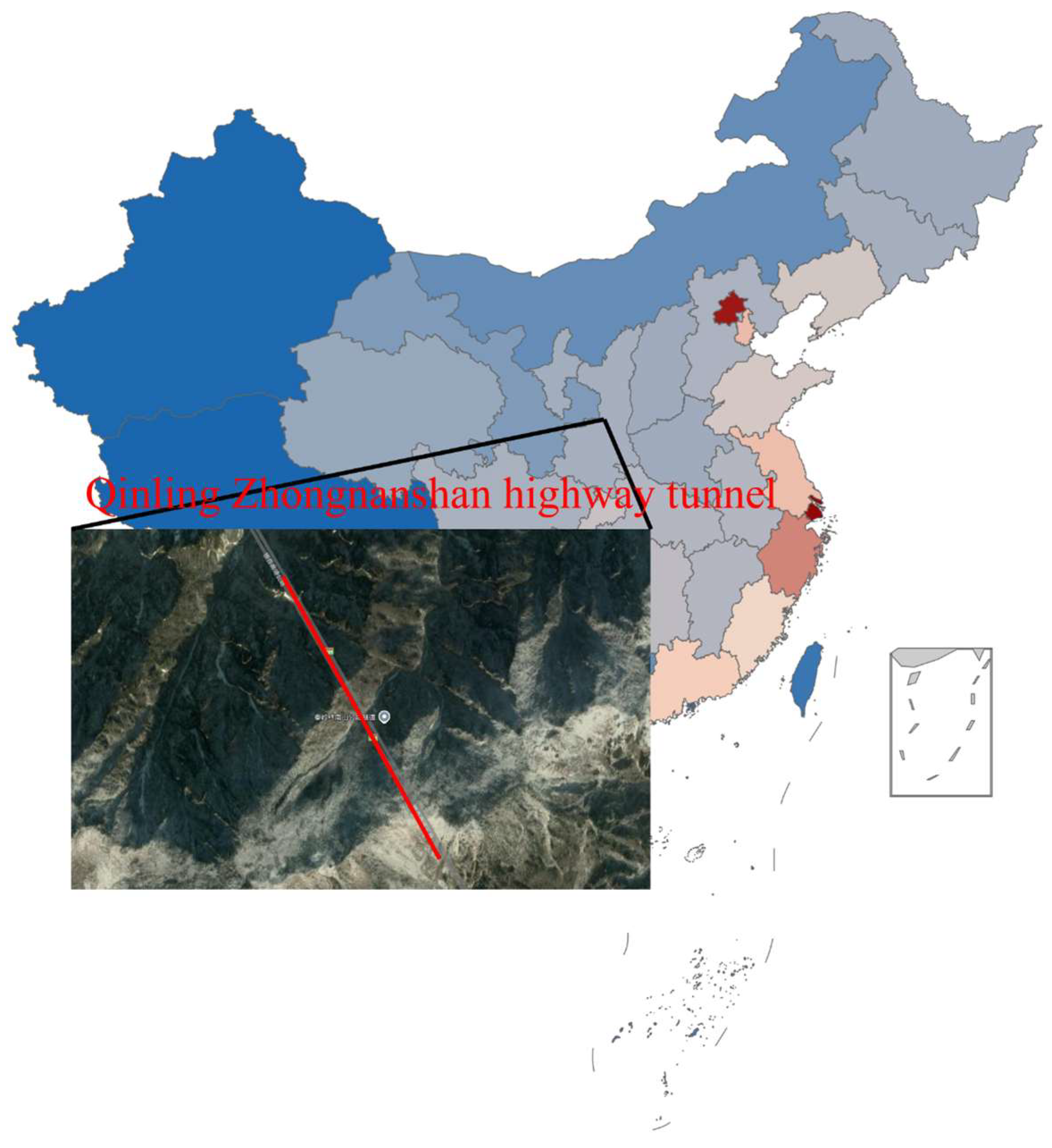
Engineering cases from Wang [34] were used to validate the reliability of the proposed model, as shown in Figure 13. The Zhongnanshan Highway Tunnel extends for 18.02 km and incorporates a longitudinal ventilation system utilizing three shafts. Notably, Shaft No. 2 is positioned approximately 30 m upstream of the midpoint of Shuidongzi Ditch on the northern slope of the Qinling Mountains. The upper 30 m of the shaft passes through Quaternary Holocene slope alluvial deposits, where the surface material consists primarily of avalanche-derived blocky soil interbedded with mixed gneiss, classified as type II surrounding rock. Below this, the geological formation transitions into mixed gneiss, with certain sections containing remnants of obliquely oriented amphibole gneiss enriched with biotite. The lower rock mass is largely intact, classified as type VI surrounding rock, exhibiting minimal structural disturbance. In zones with greater burial depth, the measured maximum horizontal principal stress reaches 21.04 MPa, oriented NW28°, indicative of a high in situ stress environment with a pronounced potential for rockburst occurrence.
The rockburst hazards of the Zhongnanshan Tunnel were predicted by the BSLO-RF model, and the results are shown in Table 4. The BSLO-RF model utilizes the blood-sucking leech optimizer (BSLO) to optimize the hyperparameters of the Random Forest (RF) algorithm, aiming to enhance the model’s predictive accuracy and generalization ability in complex geological environments.
As presented in Table 4, the prediction results obtained by the BSLO-RF model generally match well with the actual engineering records. Among the five prediction instances, four cases exhibited perfect consistency between the predicted rockburst hazard levels and the actual recorded hazard levels, demonstrating the strong reliability and accuracy of the BSLO-RF model in practical applications. However, a prediction deviation was identified in instance 1. In this case, the actual recorded rockburst hazard level was II, whereas the BSLO-RF model classified it as level III. This deviation can be attributed to several factors. First, potential noise or outliers in the dataset may have affected the model’s ability to accurately capture the true rockburst behavior in this specific case. Second, although the k-medoids-SMOTE technique was employed during data preprocessing to address the class imbalance problem, the introduction of synthetic samples may not have fully represented the complexity of the real geological conditions. This could have resulted in reduced generalization ability of the model in certain borderline cases.
Despite this isolated prediction deviation, the BSLO-RF model demonstrated excellent overall predictive performance. The consistent prediction results across most instances indicate that the BSLO-RF model effectively captures the nonlinear relationships between rock mechanical properties and rockburst hazard levels. Furthermore, the integration of the BSLO algorithm significantly improved the RF model’s optimization efficiency, enabling better feature selection and parameter tuning. Based on the above analysis, it can be concluded that the BSLO-RF model provides an effective and practical tool for rockburst hazard prediction in tunnel engineering. Its robust performance in the Zhongnanshan Tunnel case study demonstrates its potential for broader applications in complex and high-risk geological environments.

5. Conclusions

This study developed an intelligent rockburst intensity prediction framework by integrating the k-medoids-SMOTE data balancing method with a blood-sucking leech optimizer-enhanced Random Forest (BSLO-RF) model. The main conclusions are as follows:
(1)
A dataset of 351 documented rockburst cases was compiled and classified into four intensity levels. Data imbalance and outlier effects were mitigated using z-score normalization and k-medoids-SMOTE, improving inter-class separability.
(2)
The BSLO algorithm effectively tuned Random Forest hyperparameters, enhancing classification accuracy, recall, and F1-score compared with conventional methods. On the balanced dataset, the BSLO-RF model achieved an average accuracy of 89.16%, with notable improvements in extreme-grade prediction.
(3)
Application to the Zhongnanshan Tunnel project achieved 80% prediction accuracy, verifying the model’s robustness and adaptability in complex geological conditions.
Future research will (1) integrate real-time monitoring data to enable dynamic, time-sensitive hazard warnings; (2) expand datasets to cover diverse geological contexts and incorporate multi-source heterogeneous data for improved generalization; and (3) refine BSLO’s adaptability to high-dimensional feature spaces and explore its integration with advanced deep learning models to capture complex nonlinear relationships.

Author Contributions

Conceptualization, Q.W., B.D., D.L., H.J. and P.L.; methodology, Q.W., B.D., D.L., H.J. and P.L.; software, Q.W., B.D. and D.L.; validation, D.L., H.J. and P.L.; formal analysis, D.L., H.J. and P.L.; investigation, Q.W., B.D. and H.J.; resources, B.D., D.L. and P.L.; data curation, Q.W. and H.J.; writing—original draft preparation, D.L. and P.L.; writing—review and editing, Q.W. and P.L.; visualization, Q.W., B.D. and H.J.; supervision, D.L. and P.L.; project administration, Q.W., B.D. and H.J. All authors have read and agreed to the published version of the manuscript.

Funding

This research was funded by the National Science and Technology Major Project (Grant No. 2024ZD1001906), the National Natural Science Foundation of China (Grant No. 52204128), and the Natural Science Foundation of Shandong Province (Grant No. ZR2024QE103).

Data Availability Statement

All data can be obtained by emailing the corresponding author.

Conflicts of Interest

Author Qinzheng Wu was employed by the company Deep Mining Laboratory of Shandong Gold Group Co., Ltd. The remaining authors declare that the research was conducted in the absence of any commercial or financial relationships that could be construed as a potential conflict of interest.

References

  1. Liang, W.; Zhao, G.; Wu, H.; Dai, B. Risk Assessment of Rockburst via an Extended MABAC Method under Fuzzy Environment. Tunn. Undergr. Space Technol. 2019, 83, 533–544. [Google Scholar] [CrossRef]
  2. Zhai, S.; Su, G.; Yin, S.; Zhao, B.; Yan, L. Rockburst Characteristics of Several Hard Brittle Rocks: A True Triaxial Experimental Study. J. Rock. Mech. Geotech. Eng. 2020, 12, 279–296. [Google Scholar] [CrossRef]
  3. Ma, C.S.; Chen, W.Z.; Tan, X.J.; Tian, H.M.; Yang, J.P.; Yu, J.X. Novel Rockburst Criterion Based on the TBM Tunnel Construction of the Neelum–Jhelum (NJ) Hydroelectric Project in Pakistan. Tunn. Undergr. Space Technol. 2018, 81, 391–402. [Google Scholar] [CrossRef]
  4. Barton, N. Some New Q-Value Correlations to Assist in Site Characterisation and Tunnel Design. Int. J. Rock. Mech. Min. Sci. 2002, 39, 185–216. [Google Scholar] [CrossRef]
  5. Malan, D.F.; Napier, J.A.L. Rockburst Support in Shallow-Dipping Tabular Stopes at Great Depth. Int. J. Rock. Mech. Min. Sci. 2018, 112, 302–312. [Google Scholar] [CrossRef]
  6. Gong, F.; Wang, Y.; Luo, S. Rockburst Proneness Criteria for Rock Materials: Review and New Insights. J. Cent. South. Univ. Technol. 2020, 27, 2793–2821. [Google Scholar] [CrossRef]
  7. Ghasemi, E.; Gholizadeh, H.; Adoko, A.C. Evaluation of Rockburst Occurrence and Intensity in Underground Structures Using Decision Tree Approach. Eng. Comput. 2020, 36, 213–225. [Google Scholar] [CrossRef]
  8. Li, N.; Feng, X.; Jimenez, R. Predicting Rock Burst Hazard with Incomplete Data Using Bayesian Networks. Tunn. Undergr. Space Technol. 2017, 61, 61–70. [Google Scholar] [CrossRef]
  9. Qiu, Y.; Zhou, J. Short-Term Rockburst Damage Assessment in Burst-Prone Mines: An Explainable XGBOOST Hybrid Model with SCSO Algorithm. Rock Mech. Rock Eng. 2023, 56, 8745–8770. [Google Scholar] [CrossRef]
  10. Sun, L.; Hu, N.; Ye, Y.; Tan, W.; Wu, M.; Wang, X.; Huang, Z. Ensemble Stacking Rockburst Prediction Model Based on Yeo–Johnson, K-Means SMOTE, and Optimal Rockburst Feature Dimension Determination. Sci. Rep. 2022, 12, 15352. [Google Scholar] [CrossRef]
  11. Zhou, J.; Yang, P.; Peng, P.; Khandelwal, M.; Qiu, Y. Performance Evaluation of Rockburst Prediction Based on PSO-SVM, HHO-SVM, and MFO-SVM Hybrid Models. Min. Met. Explor. 2023, 40, 617–635. [Google Scholar] [CrossRef]
  12. Li, D.; Liu, Z.; Armaghani, D.J.; Xiao, P.; Zhou, J. Novel Ensemble Tree Solution for Rockburst Prediction Using Deep Forest. Mathematics 2022, 10, 787. [Google Scholar] [CrossRef]
  13. Tang, Y.; Yang, J.; Wang, S.; Wang, S. Analysis of Rock Cuttability Based on Excavation Parameters of TBM. Geomech. Geophys. Geo-Energy Geo-Resour. 2023, 9, 93. [Google Scholar] [CrossRef]
  14. Cook, N.G.W.; Hoek, E.; Pretorius, J.P.G.; Ortlepp, W.D.; Salamon, H.D.G. Rock Mechanics Applied to the Study of Rockbursts. J. South. Afr. Inst. Min. Metallurgy. 1966, 66, 435–528. [Google Scholar]
  15. Aubertin, M.; Gill, D.; Simon, R. On the Use of the Brittleness Index Modified (BIM) to Estimate the Post-Peak Behavior of Rocks. 1994. Available online: https://scispace.com/papers/on-the-use-of-the-brittleness-index-modified-bim-to-estimate-3ckb47y2cn (accessed on 5 August 2025).
  16. Brown, E.T.; Hoek, E. Underground Excavations in Rock; CRC Press: Boca Raton, FL, USA, 1980; ISBN 1-4822-8892-3. [Google Scholar]
  17. Tao, Z.Y. Rockburst in High Ground Stress Area and Its Identification. People’s Yangtze River 1987, 4, 25–32. [Google Scholar]
  18. Li, D.; Chen, Y.; Dai, B.; Wang, Z.; Liang, H. Numerical Study of Dig Sequence Effects during Large-Scale Excavation. Appl. Sci. 2023, 13, 11342. [Google Scholar] [CrossRef]
  19. Pu, Y.; Apel, D.B.; Liu, V.; Mitri, H. Machine Learning Methods for Rockburst Prediction-State-of-the-Art Review. Int. J. Min. Sci. Technol. 2019, 29, 565–570. [Google Scholar] [CrossRef]
  20. Xue, Y.; Bai, C.; Qiu, D.; Kong, F.; Li, Z. Predicting Rockburst with Database Using Particle Swarm Optimization and Extreme Learning Machine. Tunn. Undergr. Space Technol. 2020, 98, 103287. [Google Scholar] [CrossRef]
  21. Yin, X.; Liu, Q.; Huang, X.; Pan, Y. Real-Time Prediction of Rockburst Intensity Using an Integrated CNN-Adam-BO Algorithm Based on Microseismic Data and Its Engineering Application. Tunn. Undergr. Space Technol. 2021, 117, 104133. [Google Scholar] [CrossRef]
  22. Ullah, B.; Kamran, M.; Rui, Y. Predictive Modeling of Short-Term Rockburst for the Stability of Subsurface Structures Using Machine Learning Approaches: T-SNE, K-Means Clustering and XGBoost. Mathematics 2022, 10, 449. [Google Scholar] [CrossRef]
  23. Liu, Y.; Hou, S. Rockburst Prediction Based on Particle Swarm Optimization and Machine Learning Algorithm. In Proceedings of the 3rd International Conference on Information Technology in Geo-Engineering, Guimarães, Portugal, 29 September–2 October 2019; Springer Nature: Berlin/Heidelberg, Germany, 2020; pp. 292–303. [Google Scholar] [CrossRef]
  24. Qiu, D.; Li, X.; Xue, Y.; Fu, K.; Zhang, W.; Shao, T.; Fu, Y. Analysis and Prediction of Rockburst Intensity Using Improved DS Evidence Theory Based on Multiple Machine Learning Algorithms. Tunn. Undergr. Space Technol. 2023, 140, 105331. [Google Scholar] [CrossRef]
  25. Sun, Y.; Li, G.; Yang, S. Rockburst Interpretation by a Data-Driven Approach: A Comparative Study. Mathematics 2021, 9, 2965. [Google Scholar] [CrossRef]
  26. Zhou, J.; Guo, H.; Koopialipoor, M.; Jahed Armaghani, D.; Tahir, M.M. Investigating the Effective Parameters on the Risk Levels of Rockburst Phenomena by Developing a Hybrid Heuristic Algorithm. Eng. Comput. 2021, 37, 1679–1694. [Google Scholar] [CrossRef]
  27. Ma, K.; Shen, Q.-q.; Sun, X.-y.; Ma, T.-h.; Hu, J.; Tang, C.-a. Rockburst prediction model using machine learning based on microseismic parameters of Qinling water conveyance tunnel. J. Cent. South. Univ. 2023, 30, 289–305. [Google Scholar] [CrossRef]
  28. Liu, R.; Ye, Y.; Hu, N.; Chen, H.; Wang, X. Classified Prediction Model of Rockburst Using Rough Sets-Normal Cloud. Neural Comput. Appl. 2019, 31, 8185–8193. [Google Scholar] [CrossRef]
  29. Pu, Y.; Apel, D.B.; Xu, H. Rockburst Prediction in Kimberlite with Unsupervised Learning Method and Support Vector Classifier. Tunn. Undergr. Space Technol. 2019, 90, 12–18. [Google Scholar] [CrossRef]
  30. Xue, Y.; Bai, C.; Kong, F.; Qiu, D.; Li, L.; Su, M.; Zhao, Y. A Two-Step Comprehensive Evaluation Model for Rockburst Prediction Based on Multiple Empirical Criteria. Eng. Geol. 2020, 268, 105515. [Google Scholar] [CrossRef]
  31. Gong, F.; Dai, J.; Xu, L. A Strength-Stress Coupling Criterion for Rockburst: Inspirations from 1114 Rockburst Cases in 197 Underground Rock Projects. Tunn. Undergr. Space Technol. 2023, 142, 105396. [Google Scholar] [CrossRef]
  32. Wang, J.; Ma, H.; Yan, X. Rockburst Intensity Classification Prediction Based on Multi-Model Ensemble Learning Algorithms. Mathematics 2023, 11, 838. [Google Scholar] [CrossRef]
  33. Bai, J.; Nguyen-Xuan, H.; Atroshchenko, E.; Kosec, G.; Wang, L.; Abdel Wahab, M. Blood-Sucking Leech Optimizer. Adv. Eng. Softw. 2024, 195, 103696. [Google Scholar] [CrossRef]
  34. Yu, W.; Xu, Q. Rock Burst Prediction in Deep Shaft Based on RBF-AR Model. J. Jilin Univ. 2013, 43, 1943–1949. [Google Scholar]
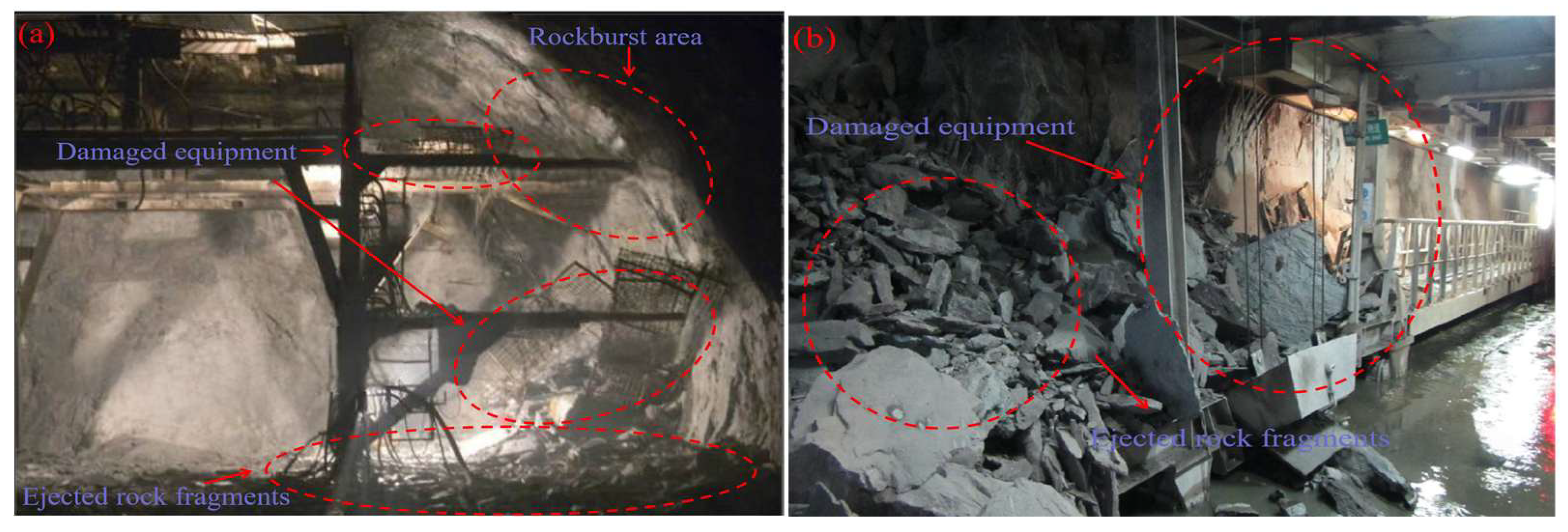
Figure 1. Photos of rockburst occurrence: (a) Damaged operating platform [9], (b) Diversion tunnel in Pakistan [10].
Applsci 15 09045 g001
Figure 2. Spatial and temporal distribution of rockburst cases in China, Data source: [11,12].
Applsci 15 09045 g002
Figure 3. Distribution of rockburst intensity grade data.
Applsci 15 09045 g003
Figure 4. Scatter box semi-violin diagram of rockburst prediction index system. Statistical validation: One-way ANOVA was performed to assess parameter distributions across rockburst grades, confirming significant differences between all intensity levels (p < 0.01 for all parameters). σ c ,   σ t , and W e t exhibit the strongest discriminatory power (F-statistics: 32.6, 28.9, 25.3), validating their role as core indicators for rockburst intensity classification. The visualization integrates boxplots (interquartile ranges), scatter plots (raw data), and half-violin plots (kernel density) to comprehensively reflect data distribution characteristics.
Applsci 15 09045 g004
Figure 5. Distribution of the original data after it is reduced to three-dimensional space.
Applsci 15 09045 g005
Figure 6. Distribution of pre-treated rockburst data after dimensionality reduction to three-dimensional space.
Applsci 15 09045 g006
Figure 7. Flowchart of BSL-RF model construction.
Applsci 15 09045 g007
Figure 8. BSLO fitness.
Applsci 15 09045 g008
Figure 9. Test set confusion matrix. X-axis: predicted grades (1–4 correspond to Class I–IV); Y-axis: actual grades. For BSLO-RF, misclassification of Class III (moderate rockburst) primarily occurs with Class II (18%), attributed to overlapping σθ/σc distributions (mean: 0.45 for III vs. 0.50 for II, Table 1). BSLO-DT shows poor performance for Class II (40% accuracy), reflecting its inability to capture nonlinear relationships between stress ratios and rockburst intensity. (a) BSLO-BP; (b) BSLO-CNN; (c) BSLO-DT; (d) BSLO-RF; (e) BSLO-SVM.
Applsci 15 09045 g009
Figure 10. Year-on-year deviation chart. Year-on-year performance improvement after BSLO optimization. ‘Relative improvement’ is calculated as (Post-optimization—Pre-optimization)/Pre-optimization × 100%. BSLO-BP shows the most significant gain (36.68% in accuracy) because BSLO’s ‘Re-tracking Strategy’ mitigates BP’s tendency to fall into local optima. BSLO-RF exhibits modest improvement (9.36%) due to RF’s inherent ensemble robustness, though BSLO still refines hyperparameters (e.g., number of decision trees = 60) for better generalization. (a) Accuracy; (b) Precision; (c) Recall; (d) F1.
Applsci 15 09045 g010
Figure 11. Comparison chart of each model before and after data preprocessing. Model performance before (raw data: Class I:II:III:IV ≈ 1.5:2.5:4.3:1.7) and after (k-medoids-SMOTE balanced data: 150 samples/grade) preprocessing. BSLO-DT shows the largest F1-score improvement (+45%, from 0.42 to 0.61), as 100 synthetic samples (generated via k-medoids cluster centers) alleviate bias toward majority classes. BSLO-RF shows milder improvement (+8%) due to its intrinsic resilience to imbalanced data. (a) BSLO-BP; (b) BSLO-CNN; (c) BSLO-DT; (d) BSLO-RF; (e) BSLO-SVM.
Applsci 15 09045 g011
Figure 12. Contributions of various model variables. (a) BSLO-CNN; (b) BSLO-CNN; (c) BSLO-DT; (d) BSLO-RF; (e) BSLO-SVM.
Applsci 15 09045 g012
Figure 13. Geographical locations of the engineering cases.
Applsci 15 09045 g013
Table 1. Statistical parameters of different rockburst grades.
Rockburst GradeRockburst Characteristic Parameters
Statistical Parameter σ c (MPa) σ t (MPa) σ θ (MPa) σ θ / σ c σ c / σ t Wet (MJ/m3)
NoneMaximum value241.0018.50107.505.2648.217.90
Minimum value18.320.381.600.085.701.10
Mean value115.555.3726.130.4027.013.74
Coefficient of variation0.490.720.752.420.470.62
LightMaximum value263.0018.20148.404.5542.9610.00
Minimum value26.060.7710.900.094.481.80
Mean value130.186.0753.070.5024.684.39
Coefficient of variation0.380.520.521.220.360.43
ModerateMaximum value304.0019.20132.102.5780.0010.00
Minimum value30.001.4310.360.089.741.20
Mean value141.006.9660.410.4523.265.17
Coefficient of variation0.330.460.430.520.470.34
StrongMaximum value306.5820.99167.201.7280.0011.62
Minimum value30.001.5012.360.0810.762.03
Mean value150.597.9675.630.5424.846.22
Coefficient of variation0.340.520.440.520.730.28
Note: The large differences between maximum and minimum values are typical of rockburst datasets, reflecting variability in geological conditions (e.g., lithology, in situ stress) across engineering sites [31]. Despite this dispersion (coefficient of variation: 0.28–2.42), mean values remain statistically meaningful, as confirmed by consistent median values (Level I: 112.6 MPa; Level II: 128.5 MPa; Level III: 139.8 MPa; Level IV: 148.2 MPa). This alignment validates the use of mean values to represent overall trends.
Table 2. High-Level Workflow of BSLO.
StepKey OperationBiological AnalogyPurpose
1Initialize population with two types of individuals: directional leeches (sensitive to environmental cues) and directionless leeches (limited perception).Leeches scatter across the rice field to maximize coverage.Cover the entire solution space to avoid missing potential optima.
2Update positions of directional leeches based on the current optimal solution.Leeches move toward detected hosts using sensory signals.Rapidly converge toward promising regions in the search space.
3Update positions of directionless leeches via random walks (Lévy flight).Leeches wander randomly after being disturbed by the host.Refine local search to exploit details around potential optima.
4Calculate Perceived Distance (PD) to switch between exploration (PD > 1) and exploitation (PD ≤ 1) modes.Leeches adjust behavior based on proximity to the host (far: explore broadly; near: focus locally).Dynamically balance global and local search to prevent premature convergence.
5Trigger re-tracking strategy: Re-initialize positions of leeches that stagnate (no improvement after t1 iterations compared to t2 prior steps).Leeches relocate to new areas if they fail to find prey for too long.Escape local optima and maintain search diversity.
6Repeat steps 2–5 until maximum iterations (T) are reached.Sustained foraging cycles to ensure thorough exploration.Output the globally optimal solution.
Table 3. Classification performance metrics of models on the test set (mean ± standard deviation).
ModelAccuracyRecallF1-ScoreAccuracy (Class I)Accuracy (Class IV)
BSLO-RF(89.16 ± 1.23)%(87.5 ± 1.56)%0.88 ± 0.0293.3%87.9%
BSLO-SVM(82.45 ± 1.89)%(80.1 ± 2.11)%0.81 ± 0.0393.3%75.8%
BSLO-BP(77.50 ± 2.34)%(75. ± 2.56)%0.76 ± 0.04100%72.7%
BSLO-CNN(72.33 ± 2.67)%(70.58 ± 2.89)%0.71 ± 0.0590%66.6%
BSLO-DT(65.21 ± 3.12)%(63.15 ± 3.22)%0.64 ± 0.0690%69.7%
Table 4. Prediction results obtained by the proposed models.
NO.ProvenanceUCS
(MPa)
UTS
(MPa)
MTS
(MPa)
MTS/UCSUCS/
UTS
W e t
(MJ/m3)
Rockburst Hazard
Engineering
Records
BSLO-RF
1Zhongnanshan Tunnel1225.3843.10.3522.683.31Ⅲ *
2Zhongnanshan Tunnel1218.7387.50.7213.869.05
3Zhongnanshan Tunnel1248.6479.10.6414.357.74
4Zhongnanshan Tunnel1197.2156.20.4716.55.52
5Zhongnanshan Tunnel1206.4562.80.5218.64.16
* The flag of prediction error.
Disclaimer/Publisher’s Note: The statements, opinions and data contained in all publications are solely those of the individual author(s) and contributor(s) and not of MDPI and/or the editor(s). MDPI and/or the editor(s) disclaim responsibility for any injury to people or property resulting from any ideas, methods, instructions or products referred to in the content.