Abstract
Kolmogorov–Arnold Networks (KANs) have recently emerged as a powerful alternative to traditional Artificial Neural Networks (ANNs), offering superior accuracy and interpretability, which are two critical requirements in healthcare applications. This study investigates the effectiveness of KANs across a range of clinical tasks by applying them to diverse medical datasets, including structured clinical data and time-series physiological signals. Compared with conventional ANNs, KANs demonstrate significantly improved performance, achieving higher predictive accuracy even with smaller network architectures. Beyond performance gains, KANs offer a unique advantage: the ability to extract symbolic expressions from learned functions, enabling transparent, human-interpretable models—a key factor in clinical decision-making. Through comprehensive experiments and symbolic analysis, our results reveal that KANs not only outperform ANNs in modeling complex healthcare data but also provide interpretable insights that can support personalized medicine and early diagnosis. There is nothing specific about the datasets or the methods employed, so the findings are broadly applicable and position KANs as a compelling architecture for the future of AI in healthcare.
1. Introduction
The application of artificial intelligence (AI) in healthcare has experienced a transformative rise in recent years, driven by the need for more accurate, efficient, and interpretable decision-support systems. Traditional deep learning models, particularly Artificial Neural Networks (ANNs), have demonstrated impressive performance across various tasks such as disease diagnosis, prognosis prediction, and patient monitoring. They often detect patterns that are not readily apparent to the human senses. However, these models often suffer from a lack of interpretability and are prone to overfitting, especially when applied to small or noisy datasets typical of clinical settings.
Kolmogorov–Arnold Networks (KANs) have emerged as a promising alternative to conventional ANNs. Continued research into interpretable architectures like KANs could help alleviate concerns around AI’s environmental impact, opaque decision-making, and ethical governance [1]. Rooted in the Kolmogorov–Arnold representation theorem, KANs replace fixed activation functions with learnable univariate functions, offering a novel approach to modeling nonlinear relationships. This paradigm shift enhances both the expressive power and interpretability of neural models. KANs are especially appealing in healthcare, where transparency, explainability, and robustness are paramount for clinical trust and adoption. In healthcare and particularly mental health, relying solely on model evaluation metrics without the backing of interpretations based on explainability techniques can be dangerous [2].
This study aims to investigate whether Kolmogorov–Arnold Networks (KANs) can consistently outperform traditional Artificial Neural Networks (ANNs) in healthcare tasks in terms of predictive accuracy, interpretability, and robustness across diverse healthcare datasets. We assess classification performance using accuracy, AUC, and F1 score, and regression performance using MSE, MAE, and R2 while examining KAN’s symbolic explainability and computational efficiency.
1.1. Related Work
Kolmogorov–Arnold Networks (KANs) are particularly gaining attention for applications that need both interpretability and accuracy. Unlike typical neural networks, which use fixed activation functions at each node (as in Multi-Layer Perceptrons), KANs shift this to the edges by allowing learnable activation functions. This shift [3] will improve both performance and clarity of the model, thereby making it more suitable for healthcare applications.
There has been a recent surge in exploring the application of KANs across various healthcare-related tasks. For example, specialized architectures such as Chebyshev Polynomial-Based KANs [4] have been designed to improve how well a network can fit polynomial functions and also be more computationally efficient, thus emphasizing their importance in medical data processing [5]. In addition, the Kolmogorov–Arnold Network, which involves physics-informed principles, shows significant ways of solving partial differential equations (PDEs) related to biomedical applications [6,7]. A Thermodynamic Kolmogorov–Arnold Model (TKAM) further extends this by integrating thermodynamic constraints into KAN’s architecture for structured probabilistic modeling [8].
Applications in Medical Imaging and Time Series Analysis: KANs have demonstrated significant potential in medical imaging, particularly in the production and classification of medical images. For example, U-KAN, a KAN variant designed especially for medical image analysis, performs better in segmentation tasks than traditional convolutional neural networks (CNNs), thereby providing more precise diagnostic tools [9].
KANs have shown great results in the field of time series analysis. By accurately capturing temporal dependencies better than conventional techniques, temporal KANs (TKANs) provide strong frameworks for time series forecasting, which is significant in the healthcare industry in preparing for medical outcomes [6]. Replacing linear weights with spline-parametrized univariate functions has proven to yield more accurate and parameter-efficient time-series forecasts on real-world traffic data [10]. Fractional Kolmogorov–Arnold Networks (fKANs) have further shown increased predictive modeling performance, particularly in patient forecasting, highlighting their use in predictive analytics for healthcare [11].
Explainability and Symbolic Regression in Healthcare: The explainability of KANs is a huge advantage in the healthcare industry, as it helps us to understand how the models make their decisions. Research has employed post-hoc explainability techniques like integrated gradients, SHAP, and LIME to explain KAN decision-making. These techniques have been used in medical datasets, which shows that KANs not only give better accuracy but also offer clearer insights into model choices [12].
Moreover, the symbolic regression capabilities of KANs have opened new possibilities for extracting mathematical and physical rules from healthcare data. A recent study demonstrated how KANs can help in rediscovering known medical formulas and potentially discovering new ones, thus making them valuable tools in medical research [13].
Emerging Applications and Future Directions: KANs aren’t just useful in healthcare; they’re starting to show potential in many other fields as well [14]. For instance, Wav-KAN, which combines wavelet transforms with KANs, has shown better results in signal processing. This can be helpful when working with biomedical signals like ECG or EEG data [15]. On top of that, researchers are developing convolutional KANs, which could significantly improve how we extract features from complex medical images. Graph KANs carry the spline trick over to network data by learning a simple curve on each connection, and this tweak delivers standout gains on node-classification tasks [16]. Also, KANICE augments KANs with interactive convolutional elements, combining CNN-style spatial feature extraction with KAN’s spline activations for vision tasks [17]. All of these points point to new ways KANs can contribute to advancements in healthcare [18].
Recent progress in using KANs for reinforcement learning and even in quantum computing shows that they could become an integral part of future AI-powered healthcare technologies [19]. Another paper dealing with KKANs, Kurkova–Kolmogorov–Arnold Networks, was introduced, exploring their learning dynamics and demonstrating faster convergence and improved stability on challenging function-approximation tasks [20]. These breakthroughs reflect a growing interest in applying KANs to a wide variety of areas with the potential to transform healthcare and other fields [21].
1.2. Contribution
In this paper, we try to make key contributions to the study of Kolmogorov–Arnold Networks (KANs) in the healthcare field:
- Comparison with traditional ANNs: We compared KANs with traditional Artificial Neural Networks (ANNs) to see how they stack up in terms of accuracy, interpretability, and efficiency. The results showed that KANs outperformed ANNs in all these aspects, even when using smaller network setups.
- Generalizable findings: The study’s methodologies and conclusions are not tied to any specific dataset or method. This generalization proves that KANs can be broadly applied across the healthcare domain.
- Contribution to healthcare AI: By proving KANs’ effectiveness in healthcare applications, we try to deliver insights that can help shape future research and development of AI models that require high accuracy and interpretability, which are essential in the medical field.
2. Materials and Methods
In this study, we aim to evaluate how effective Kolmogorov–Arnold Networks (KANs) are in the healthcare domain using a methodical and reproducible approach, which has the potential to be explored further. To this effect, we designed a comparative methodology involving both classification and regression tasks. The datasets were preprocessed using standard techniques, including normalization, imputation of missing values, and feature selection through recursive feature elimination (RFE) and signal transformation methods like wavelet decomposition. KANs were implemented based on the Kolmogorov–Arnold representation theorem, utilizing spline-based learnable functions in place of traditional activation functions. For benchmarking, conventional Artificial Neural Networks (ANNs) were trained using equivalent data splits and tuned hyperparameters. Both models were evaluated using appropriate metrics—accuracy, precision, recall, and F1 score for classification tasks, and mean squared error (MSE), mean absolute error (MAE), and for regression. Special emphasis was placed on interpretability by extracting symbolic expressions from the trained KANs, offering insights into the underlying data relationships critical in clinical decision-making.
2.1. Datasets
In this study, four publicly available healthcare datasets were selected to evaluate the performance of Kolmogorov–Arnold Networks (KANs) across both classification and regression tasks. The Heart Disease and Indian Liver Patient datasets represent structured clinical data and are widely used benchmarks for binary classification problems in medical diagnostics. To assess the model’s ability to capture temporal patterns, we included two time-series datasets: Continuous Glucose Monitoring (CGM) data for predicting hypoglycemic events in diabetic patients. This diverse selection ensures a comprehensive evaluation of KANs’ effectiveness across different data modalities and clinical scenarios, highlighting their potential for broad application in healthcare analytics.
- Heart Disease Dataset: This dataset contains 303 patient records, each with 14 attributes which include age, sex, chest pain type, resting blood pressure, cholesterol level, fasting blood sugar, electrocardiographic results, maximum heart rate achieved, exercise-induced angina, oldpeak (ST depression induced by exercise relative to rest), slope of peak exercise ST segment, number of major vessels colored by fluoroscopy, and a class label indicating the presence or absence of heart disease.
- Indian Liver Patient Dataset: This dataset includes 583 records with 11 features, which are associated with liver function like total bilirubin, direct bilirubin, alkaline phosphatase, alanine aminotransferase, aspartate aminotransferase, total proteins, albumin, and albumin-to-globulin ratio. The binary class label shows if a patient has liver disease or not.
- Continuous Glucose Monitoring (CGM) Dataset: This dataset includes time-series data collected from diabetic patients, capturing glucose levels at a 5 min interval for approximately 2.5 h. The dataset was preprocessed to remove faulty readings and normalize the values.
2.2. Data Preprocessing
The pre-processing steps are defined below.
- Missing values in the Heart Disease and Indian Liver Patient datasets were imputed using the mean for continuous variables and the mode for categorical variables. For time-series data in the CGM dataset, linear interpolation was used to fill the missing values. Since only the final time step was missing in a small number, and the glucose level change was minimal over a 5 min interval, we used a simple linear interpolation to efficiently impute those tail values.
- Continuous variables in all the datasets were normalized using appropriate scaling techniques. MinMaxScaler (scikit-learn v1.3.2) was applied for the CGM and Heart datasets, while RobustScaler was used for the Liver dataset to mitigate the effect of outliers. Time-series data in the CGM dataset were also normalized on a per-patient basis to account for individual variability.
- The CGM dataset was split into separate time windows, 5 min intervals for CGM data, which captured the temporal patterns in the signals. Each of these segments was then used as an individual sample for regression tasks.
2.3. Feature Selection
Feature selection played a key role in improving the model’s performance by cutting down unnecessary data and focusing only on relevant parameters.
- RFE was employed on the Heart Disease and Indian Liver Patient datasets to select important features [22]. The RFE process was repeated with different classifiers to ensure robustness; thereby, only the top features were selected based on their importance scores.
- The selected features for the Heart dataset were 10 variables: cp, thalach, slope, restecg, age, sex, chol, trestbps, thal, and ca. For the Liver dataset, six features were retained from the original 10 predictors: age, gender, total_bilirubin, alkaline_phosphotase, alamine_aminotransferase, and albumin_and_globulin_ratio.
- For the CGM, key features like mean glucose level, glucose variability, and rate of change were extracted.
2.4. Data Splitting
The datasets were divided into training, validation, and test sets using a stratified sampling approach for the classification task, ensuring class balance across splits. For the CGM, splitting was done chronologically to reflect real-world scenarios where models are trained on historical data and evaluated on future data.
- Heart Disease and Indian Liver Patient Datasets: Heart Disease collection of 1025 patients (10 clinical features each). No up-/down-sampling was applied, since the classes are roughly balanced. The data was split into 80% for training and 20% for testing. This gave 820 training examples (evenly split into 410 healthy and 410 diseased cases) and 205 held-out tests (102 healthy vs. 103 diseased), preserving the original class balance in both sets and ensuring a fair assessment of our models.
- Indian Liver Patient Datasets: The original Indian Liver Patient Dataset comprised 583 records (416 disease, 167 no-disease). We bootstrap-upsampled the minority (no-disease) class from 167 to 416 samples, which yielded 832 total records (416 disease + 416 healthy). The data was split into 75% for training and 25% for testing on this balanced set, resulting in 624 training samples and 208 test samples, with each split containing 312 disease and 312 healthy cases in the training set and 104 disease and 104 healthy cases in the test set.
- CGM Dataset: For the CGM experiments, we used 33 continuous glucose monitoring sessions (each with 5 min readings per patient). After normalizing each series, we split by taking the first 24 points (80%) as model inputs and the final 6 points (20%) as targets, thus yielding 33 input–output pairs.
2.5. Model Development and Training
2.5.1. Theoretical Foundation of KANs
Kolmogorov–Arnold Networks (KANs) are fundamentally based on the Kolmogorov–Arnold representation theorem [3], which states that any multivariate continuous function can be broken down into a combination of a finite sum of univariate functions. This can be represented by the following equation:
In the above Equation (1) [3], and are continuous univariate functions, n represents dimensionality of the input vector x, and refers to the p-th component of x. KANs leverage this theorem by replacing traditional linear weights in neural networks with learnable univariate functions, thereby allowing more expressive and efficient approximations of complex multivariate functions. This foundational principle allows KANs to capture complex nonlinear relationships in high-dimensional data, making them more suitable for healthcare applications [11].
2.5.2. KAN Architecture
KANs take a different approach from traditional neural networks by replacing fixed linear weights with flexible, learnable functions , which are modeled using splines. This means that each neuron in a KAN layer produces its output by applying these flexible one-dimensional functions to the inputs, thereby allowing the network to capture complex patterns more effectively [3]. The output of a neuron is computed using the following Equation (2):
Here, is the output of neuron j, is the i-th input to neuron, is the learnable univariate function mapping to neuron j, and is the bias term associated with neuron j. This formula allows each neuron’s activation to be a nonlinear transformation of its inputs, thereby facilitating more flexibility [11] as compared with the traditional neural network architectures, which rely on fixed activation functions [5].
The implementation of KANs involves several components to ensure efficient training and interpretability:
- KANLayer class: This class constructs network layers where each connection is represented by a univariate function modeled with splines. These splines are initialized using adaptive grids that reflect the distribution of the input data, which allows the model to better capture important patterns by placing more knots in areas where the data is more concentrated [3].
- Symbolic_KANLayer Class: To enhance the interpretability of the model, Symbolic_KANLayer class translates learned univariate functions into symbolic expressions. These expressions offer a human-readable view of how the network processes information, which is valuable in clinical applications where understanding the model’s decision-making is crucial [11].
- Grid initialization and updates: The grids that define the spline functions are first initialized to span the entire range of the input data. As we train, these grids are periodically adjusted to better fit evolving univariate functions. The parameter grid_eps controls how these adjustments are made, striking a balance between maintaining uniform spacing and adapting knot placement based on data distribution [5]. In our experiment, we chose one global grid value for the entire network: 3 knots for the Heart model, 5 for the Liver model, and 7 for the CGM model, so that every neuron uses that same knot count and we do not mix different grid sizes within one model.
- Pruning and fine-tuning: To improve efficiency and generalization of the model, neurons and connections with low activation magnitudes are pruned by removing parts of the network that contribute little to the performance. After pruning, the remaining parameters are fine-tuned to ensure that the model continues to perform well. This process helps to maintain strong predictive accuracy while reducing computational demands and minimizing the risk of overfitting [9].
By combining these elements, the KAN architecture strikes a thoughtful balance between computational efficiency and interpretability. This makes it well-suited for handling complex challenges in healthcare data analysis, where both accuracy and transparency are essential.
2.5.3. Training Procedure
The training of Kolmogorov–Arnold Networks (KANs) follows a two-stage recipe. First, we train the full network for classification tasks; this means running LBFGS, chosen for its ability to handle large parameter spaces and converge quickly [3], for several dozen epochs. We then prune the low-impact connections and later switch to Adam using a small learning rate, light weight decay, and gradient clipping to fine-tune remaining weights. For regression tasks, we simplify things by using Adam in the beginning for a longer initial training pass, followed by pruning and a shorter Adam-based fine-tuning run under the same hyperparameters.
For optimization of KANs, different loss functions were employed based on the tasks performed:
- Classification tasks: Binary Cross-Entropy Loss () was utilized to optimize separation between classes, as this loss function measures the performance of a classification model whose output is a probability between 0 and 1.
- Regression tasks: Mean Squared Error (MSE) Loss () was employed to minimize the difference between predicted values and actual target values, as MSE is sensitive to outliers and stresses larger errors more than smaller ones.
For regularization, we applied L2 regularization through the parameter to control model complexity and prevent overfitting. This penalty discourages large weights, enhancing generalization. In addition to this, the spline-based architecture provides inherent regularization by enforcing smooth transformations and limiting abrupt changes in the learned functions. Thus, both L2 penalties and spline constraints ensure robust performance while minimizing overfitting risks.
The hyperparameters, including learning rates, regularization strengths, batch sizes, and spline grid sizes, were tuned using a grid search approach (Table 1). This systematic exploration of hyperparameter combinations was combined with cross-validation so that the selected parameters generalized well to unseen data, thereby improving the model’s robustness and performance.

Table 1.
Hyperparameter Settings for KAN and ANN Models across datasets.
KAN uses one global grid setting network-wide, so every neuron’s spline has the same knot count (e.g., grid = 3 for Heart, grid = 5 for Liver, and grid = 7 for CGM) within a single model.
To further prevent overfitting, an early stopping mechanism with a patience of 10 epochs was applied to monitor validation loss and stop training if no improvement is seen. In addition, spline grids were periodically updated during the early stages of training, allowing the model to adapt better to the data distribution and to improve its ability to capture complex patterns.
The combination of the LBFGS optimizer, carefully chosen loss functions, and strong regularization techniques ensures that KANs are trained effectively, achieving a balance between model complexity and predictive accuracy. These training strategies are essential for enabling KANs to capture complex patterns in healthcare data.
Random weight initialization was made by fixing the RNG seed as 0 for the Heart dataset and seed 123 for the Liver and CGM datasets.
2.5.4. Total Training Steps
To make sure each model’s “training effort” is comparable, we count every gradient update as one training step:
For the Heart experiments, with 242 training samples and a mini-batch size of 32, that gives steps per epoch. The Liver and CGM experiments use full-batch updates (1 step per epoch). As shown in Table 2, each model is trained for an equivalent number of gradient-update steps to ensure a fair comparison.
Table 2.
Number of gradient-update steps per model, ensuring each sees equivalent training effort.
2.5.5. Model Parameter Comparison: KAN vs. ANN
Although Kolmogorov–Arnold Networks (KANs) introduce a modest parameter overhead compared with size-matched Artificial Neural Networks (ANNs), they deliver substantially better predictive performance. Table 3 summarizes the raw parameter counts for each model across the three tasks.
Table 3.
Parameter counts for ANN and KAN architectures on each dataset.
As shown in Table 3, KANs use between 3.8× and 7.7× more parameters than their ANN counterparts. However, this additional capacity is put to good use: by embedding spline-based activation functions, KANs capture complex nonlinearities far more effectively, resulting in higher accuracy and F1-scores (see Section 3.2, Section 3.3 and Section 3.4). In practice, the slight increase in feed-forward cost is more than offset by the performance gains, yielding a superior performance-per-parameter trade-off.
2.5.6. Advantages of the KAN Code Implementation
The KAN codebase has several techniques and optimizations, especially for spline implementation. One key feature is efficient spline computation, which leverages B-spline basis functions for fast evaluation. In addition, the B_batch function enhances performance by computing these basis functions in parallel.
Another key advantage is the use of adaptive and dynamic grids, which adjust based on data distribution. This allows the model to better capture complex patterns. By continuously updating during training, the grids help to ensure the spline functions remain effective and well-aligned with the data.
Flexible activation modeling is another key strength of KANs. By representing activations as spline functions, the network can approximate a wide range of nonlinear behaviors, thereby providing greater flexibility than traditional fixed activations. Learnable spline coefficients and grids allow the model to adapt activations to the data and improve its expressive power.
Moreover, the KAN codebase includes seamless integration with PyTorch (v2.4.0) Autograd. The spline functions are fully compatible with PyTorch’s automatic differentiation, enabling smooth backpropagation through spline layers and making gradient computation and optimization more efficient.
Finally, scalability is a key advantage of KANs. Batched computations and efficient implementations enable the model to handle large datasets and complex architectures without high computational costs, thus making it well-suited for real-world, large-scale healthcare applications.
2.5.7. Symbolic Function Extraction
A key advantage of KAN is its ability to extract symbolic expressions from learned univariate functions, improving interpretability. This is very crucial in healthcare applications, as understanding variable relationships is essential.
To enable symbolic function extraction, we used the Symbolic_KANLayer class, which manages symbolic activation functions and their parameters, including input/output dimensions, function representations, and affine transformation. Key methods of the class include forward(x), which computes the layer’s output by applying affine transformations and evaluating symbolic functions; fix_symbolic(i, j, fun_name, x = None, y = None), which assigns a specific symbolic function to an activation and fits its parameters if data is provided; and get_subset(in_id, out_id), which extracts a subset of the layer for pruning, etc.
- Process of Symbolic Function Extraction Involves Four Main Steps
Step 1: For each activation function , a list of candidate symbolic functions is generated from a predefined library (e.g., sin, tanh, , ). The suggest_symbolic method evaluates each function by fitting it to the learned spline function and computes the coefficient of determination ().
Step 2: When a candidate symbolic function is selected, we fit its parameters to match the learned spline function. This involves optimizing the affine transformation parameters a, b, c, and d in Expression (3):
where f is the symbolic function [11]. The fitting process minimizes the mean squared error between outputs of the spline function and the symbolic function over input data.
Step 3: Once the spline activation function is fixed, is replaced by a symbolic function along with learned parameters using the fix_symbolic method in Symbolic_KANLayer.
Step 4: The model is updated to incorporate symbolic activations, and this process is applied for all activation functions in the network. The auto_symbolic method simplifies this by automating the procedure across the network.
In our experiments with the Heart Disease dataset, we applied a symbolic function extraction process to derive an interpretable model. The symbolic library included functions such as x, , , sqrt, tanh, sin, and abs. The extracted symbolic formula is a complex expression involving polynomial terms, hyperbolic tangent, and absolute value functions. An excerpt of the formula is:
This symbolic Expression (4) represents the nonlinear relationship between the input features and the target variable, where each term corresponds to a transformed combination of input features. It gives us a valuable insight into how different factors influence the risk of heart disease.
The extraction of symbolic functions provides several benefits:
- Interpretability: Symbolic formulas improve the transparency in the model’s decision-making process, which is essential for healthcare applications.
- Simplification: By replacing complex spline functions with simpler symbolic ones, we can reduce the model’s complexity without sacrificing performance.
- Insight into feature importance: The coefficients and terms in the symbolic expressions show the most critical features and how they interact.
Several implementation details contribute to the robustness and flexibility of the symbolic function extraction:
- Symbolic Library: A predefined set of functions is used for symbolic regression, which can be customized for a specific problem.
- SymPy Integration: The Symbolic_KANLayer uses SymPy for symbolic manipulation, thereby helping to simplify and evaluate the symbolic expressions.
- Error Handling: The implementation includes mechanisms to manage cases where fitting fails or numerical issues arise to ensure overall robustness.
2.6. Evaluation Metrics and Definitions
To assess model performance, we use widely accepted metrics from the sklearn.metrics and PyTorch libraries. Each metric is defined below, along with its mathematical formulation.
2.6.1. Binary Classification
In classification tasks where the true labels are binary (i.e., ),the model outputs logits are converted into predicted classes by applying the sigmoid function and thresholding at 0.5:
where is the sigmoid activation.
2.6.2. Classification Metrics
- Accuracy: Measures the proportion of correct predictions out of all samples.
- Precision: The proportion of predicted positive cases that are actually positive.
- Recall: The proportion of actual positive cases that were correctly identified.
- F1 score: The harmonic mean of precision and recall, used to balance both metrics.
- ROC-AUC: The Area Under the Receiver Operating Characteristic curve, summarizing the model’s ability to distinguish between classes across all thresholds.
2.6.3. Regression Metrics
- Mean Squared Error (MSE): The average of the squared differences between actual and predicted values.
- Mean Absolute Error (MAE): The average of the absolute differences between predictions and true values.
- Root Mean Squared Error (RMSE): The square root of the MSE, giving the error in the same units as the original data.
- Coefficient of Determination (): Measures how well the model explains the variance in the target variable.
These metrics collectively provide a comprehensive evaluation of our model’s performance across classification and regression tasks.
2.7. Advantages of KANs
Compared with conventional neural network architectures such as Convolutional Neural Networks (CNNs), Kolmogorov–Arnold Networks (KANs) offer notable improvements. By replacing fixed activation functions with learnable univariate functions, KANs improve both accuracy and interpretability, making them more effective for modeling complex nonlinear relationships in healthcare, where both predictive performance and transparency are critical.
Compared with MLPs, KANs demonstrate faster neural scaling, allowing them to achieve strong performance with fewer parameters. This helps reduce both overfitting and computational costs. Moreover, KANs offer improved interpretability through more intuitive visualizations and interactions, which is again very valuable for clinical decision-making.
In comparison to CNNs, which are primarily used for image-based healthcare data, KANs offer a versatile approach applicable to both structured tabular data and unstructured time-series data. This adaptability, combined with the Kolmogorov–Arnold representation theorem, makes KAN a powerful tool for a variety of healthcare applications.
3. Results and Discussion
This section presents the experimental results from applying Kolmogorov-Arnold Networks (KANs) and traditional Artificial Neural Networks (ANNs) to three datasets: the Heart Disease Dataset, the Indian Liver Patient Dataset, and the Continuous Glucose Monitoring (CGM) Dataset. The performance of both models is evaluated and discussed, highlighting the effectiveness of KANs in the healthcare domain.
3.1. Experimental Setup
The experiments were carried out using preprocessed datasets described in the Materials and Methods section. Both KAN and ANN models were trained and evaluated using the same data splits and evaluation metrics to ensure a fair comparison. For each dataset:
- Training and testing split: The datasets were split into 80% training and 20% testing subsets.
- Evaluation metrics: Accuracy, ROC AUC, F1 Score, Precision, Recall, and Classification Reports were utilized to evaluate model performance.
- Software and hardware: All experiments were implemented using Python (v3.10.12) libraries like PyTorch and TensorFlow Keras. Training was performed on a system equipped with a CUDA-enabled GPU for accelerated computation.
3.2. Heart Disease Dataset
3.2.1. KAN Model Performance
We evaluated the KAN model on the Heart Disease Dataset using the LBFGS optimizer for rapid convergence, then Adam for fine-tuning (learning rate = 0.01), and observed rapid convergence reaching optimal performance in just 2600 optimization steps. On the held-out test set, the model achieved an overall accuracy of 86.83%, a ROC AUC of 0.9269, and an F1 score of 0.8744, demonstrating both strong discriminative power and balanced class performance. Table 4 summarizes the detailed per-class precision, recall, and F1 scores:
Table 4.
Classification report for KAN model on Heart Disease Dataset (after pruning and fine-tuning).
- Interpretation
The KAN model showed superior performance on the Heart Disease Dataset, correctly classifying 86.83% of test instances. The high ROC AUC value indicates excellent discriminative ability between patients with and without heart disease. The F1 score close to 1 shows a strong balance between precision and recall.
3.2.2. ANN Model Performance
We trained a standard feed-forward ANN for 50 epochs using the Adam optimizer (learning rate = 0.001), followed by fine-tuning after pruning 20% of the model weights. On the same test split, ANN achieved an overall accuracy of 78.05%, a ROC AUC of 0.8809, and an F1 score of 0.7867, indicating reasonable but significantly lower discriminative power compared with the KAN model. Table 5 lists the detailed precision, recall, and F1 scores for each class.
Table 5.
Classification report for ANN model on Heart Disease Dataset.
- Interpretation
While the ANN model achieved reasonable performance on the Heart Disease Dataset, it significantly lagged behind the KAN model in all evaluation metrics. This highlights the superior capability of KAN in capturing complex patterns within the data.
3.3. Indian Liver Patient Dataset
3.3.1. KAN Model Performance
We trained the KAN model on the Indian Liver Patient Dataset using the same procedure as before. In spite of the inherent class imbalance and overlapping feature distributions, the model delivered strong results, achieving an overall accuracy of 85.51%, a ROC AUC of 0.8866, and an F1 score of 0.8387. Table 6 presents the detailed precision, recall, and F1 scores for each class:
Table 6.
Classification report for KAN model on Indian Liver Patient Dataset.
- Interpretation
The KAN model effectively handled the complexities of the Indian Liver Patient Dataset, achieving a balanced performance between the two classes. The high ROC AUC shows good discriminative ability.
3.3.2. ANN Model Performance
We trained the ANN model on the Indian Liver Patient dataset using LBFGS for 35 epochs, then pruned and fine-tuned with Adam for 10 epochs. After pruning and fine-tuning, the model achieved an accuracy of 53.62%, a ROC AUC of 0.6038, and an F1 score of 0.6129. Table 7 provides detailed precision, recall, and F1 score for each class.
Table 7.
Classification Report for ANN model on Indian Liver Patient Dataset.
- Interpretation
The ANN model showed lower performance compared with the KAN model, especially in terms of accuracy and F1 score. This shows that KAN’s architecture captures the underlying patterns in the liver patient data in a better fashion.
3.4. Continuous Glucose Monitoring (CGM) Dataset
3.4.1. KAN Model Performance
We evaluated the KAN model on the CGM dataset to forecast hypoglycemic events from continuous glucose measurements. The model delivered outstanding accuracy, with a mean squared error (MSE) of 0.0008, a mean absolute error (MAE) of 0.0194 and a of 0.9855 as shown in Table 8.
Table 8.
Regression Report for KAN model on CGM Dataset.
- Interpretation
In everyday terms, the pruned KAN model barely misses a beat, thus explaining almost 98% of the ups and downs in your glucose trace () and keeping its average error under 0.02. That level of precision means we can trust it to give a heads-up before the glucose dips or spikes.
3.4.2. ANN Model Performance
For comparison, the ANN model was applied to the same CGM dataset, achieving an MSE of 0.0109, an MAE of 0.0730, and an of 0.7948. Table 9 presents the full regression report:
Table 9.
Regression Report for ANN model on CGM Dataset.
- Interpretation
The ANN model did show good performance but was outperformed by the KAN model in all metrics. The results indicate that KAN’s ability to model temporal patterns and nonlinear relationships is advantageous for CGM data analysis as well.
3.5. Representative Visualizations
To give the reader an intuitive sense of how KAN and ANN behave, we include three representative plots. Figure 1 overlays the ROC curves for heart disease, Figure 2 does the same for the liver dataset, and Figure 3 shows a “spaghetti” time-series forecast vs. ground truth for one CGM patient.
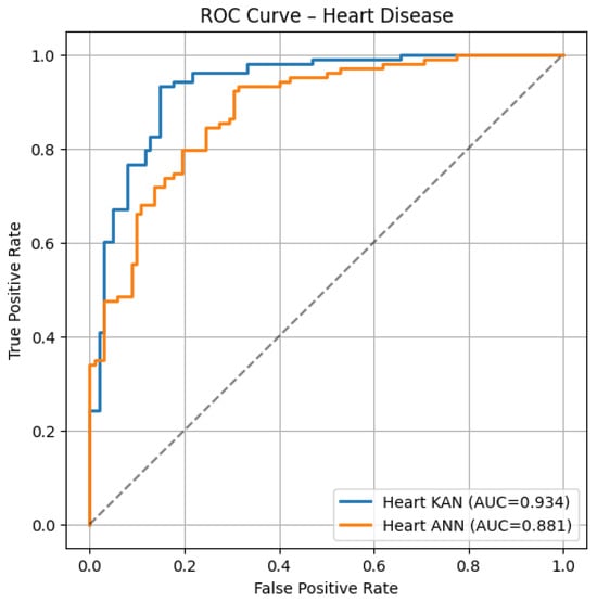
Figure 1.
ROC curves on the Heart Disease test set: KAN (blue, AUC = 0.934) vs. ANN (orange, AUC = 0.881).
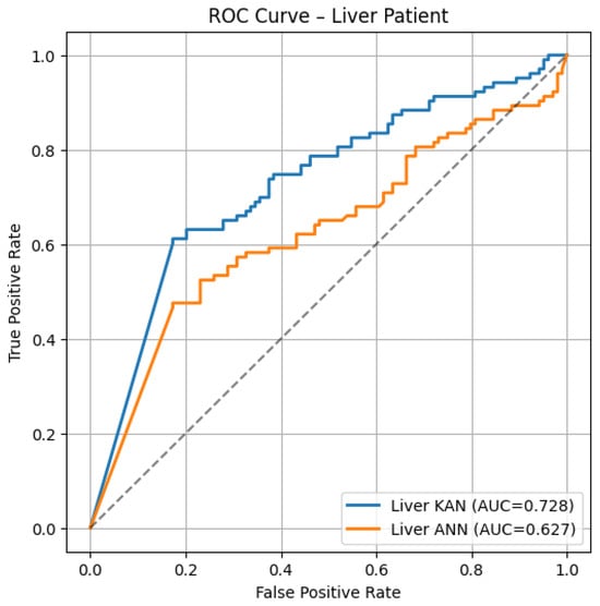
Figure 2.
ROC curves on the Liver Patient test set: KAN (blue, AUC = 0.728) vs. ANN (orange, AUC = 0.627).
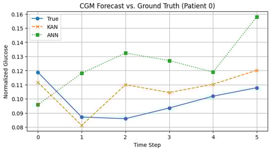
Figure 3.
CGM forecast for Patient 0: true glucose (solid), KAN (dashed), ANN (dotted).
- Heart ROC: The KAN curve remains above the ANN curve almost everywhere (AUC 0.93 vs. 0.88), suggesting stronger case separation and fewer false alarms at low false-positive rates.
- Liver ROC: Even with this liver data, which is noisy and with closer curves, KAN still does better (AUC ≈ 0.73 vs. 0.63).
- CGM Forecast: KAN’s line follows the real glucose levels closely by catching dips and slow rises, whereas ANN tends to overshoot and stay too high. Thus, KAN gives more accurate short-term predictions and avoids missing those important dips.
3.6. Comparative Analysis Across Datasets
Table 10 summarizes the comparison of the performance of ANNs and KANs on all the datasets.
Table 10.
Overall Performance Comparison of KAN and ANN Models.
- Key Observations
In terms of accuracy and ROC AUC, the KAN model continuously outperformed the ANN model across all three datasets. The superior performance of KAN demonstrates its effectiveness in modeling complex relationships within healthcare data. In addition to this, the ability of the KAN model to extract symbolic functions adds a layer of interpretability that is absent in traditional ANN models.
3.7. Statistical Significance of KAN vs. ANN Performance
To validate that the observed gains are not due to chance, we performed paired bootstrap resampling (B = 2000) on all classification and regression metrics to compute 95% confidence intervals and two-sided p-values for the difference (KAN – ANN). For the two binary tasks (Heart and Liver) we also applied McNemar’s test on per-sample predictions in this
(Heart: ; Liver: ). As summarized in Table 11, every improvement, whether it is in accuracy, F1, MSE, MAE, RMSE, or , is statistically significant, which means KAN’s performance gains over ANN are genuine and not due to chance.
Table 11.
Statistical significance of KAN vs. ANN performance differences.
3.8. Symbolic Function Analysis for the Heart Disease Dataset
The symbolic function was extracted from the trained KAN model using a simplified symbolic library that contains the functions {x, x2, x3, sqrt, tanh, sin, abs}. By fitting the learned univariate functions in the KAN model to symbolic expressions from the library, this process roughly transforms the internal representations of the model into understandable mathematical forms.
In the symbolic formula, the variables to correspond to selected features from the dataset in the following order:
- : cp (chest pain type).
- : thalach (maximum heart rate achieved).
- : slope (slope of the peak exercise ST segment).
- : age (age of the patient).
- : sex (gender of the patient).
- : thal (thalassemia).
- : ca (number of major vessels colored by fluoroscopy).
The symbolic formula that was obtained is a complex, nested expression that includes trigonometric, hyperbolic, and polynomial functions. An excerpt illustrating the structure of the symbolic function is shown below:
The symbolic formula (5) reveals several key aspects:
- Prominent functions: The hyperbolic tangent function (tanh), polynomials of degree two and three ( and ), the sine function (sin), and the absolute value function (abs) are the functions that appear most frequently. These functions indicate the nonlinear relationships in the data.
- Feature involvement: The repeated appearance of variables such as cp, thalach, slope, age, sex, thal, and ca in the formula implies that these features play a significant role in the model.
- Nested structures: The formula contains nested expressions with multiple layers of mathematical operations, including polynomials and composite functions. This complexity allows the model to capture intricate patterns and interactions between features.
- Nonlinear interactions: The use of higher-order polynomials along with nonlinear functions such as tanh and sin indicates that the model effectively captures complex, nonlinear interactions between input features and the target variable.
Analyzing specific components provides deeper insights:
- Quadratic () and Cubic () Terms: These terms suggest that the relationship between certain features and heart disease risk is nonlinear, thereby capturing effects such as thresholds or diminishing returns.For example, a cubic term like suggests that the slope of the peak exercise ST segment has a nonlinear effect on output, where both low and high values may indicate different levels of clinical risk.Similarly, a quadratic term like indicates that maximum heart rate achieved influences risk in a nonlinear manner, possibly reflecting a complex relationship between heart rate and cardiac health.
- Hyperbolic tangent (tanh) functions: The tanh function models saturation effects where increases in a feature beyond a certain point have a reduced impact on the outcome.Terms like indicate that the chest pain type influences the prediction in such a way that it levels off at higher values, thereby suggesting a threshold effect wherein certain types of chest pain significantly increase the risk, but other changes have less additional impact.
- Absolute value (abs) functions: The use of the abs functions suggests that deviations from a central value, regardless of direction, affect the outcome similarly.This could represent situations where both unusually high and low values of a feature, such as age, are associated with increased risk, highlighting the importance of maintaining features within a healthy range.
- Scaling and shifting of features: The coefficients and constants applied to the features (e.g., indicate that the model adjusts for scale and central tendency of the data, which may improve the model’s sensitivity to variations in those features.This scaling allows the model to standardize different features, thus making it easier to compare their effects, and also captures the subtle differences in patient data.
The symbolic formula highlights how the KAN model captures complex relationships in the heart disease dataset:
- Feature significance: The importance of some features in predicting heart disease is suggested by their frequent occurrences. For example, the presence of thalach (maximum heart rate achieved) in higher-order terms suggests a significant and nonlinear influence on heart disease. Increased or decreased heart rates during vigorous exercise may be a sign of underlying heart problems.
- Nonlinear effects: The model accounts for nonlinear effects that traditional linear models might miss. This is crucial in medical data, where relationships between variables and outcomes are often not exactly linear. The higher-order terms in the symbolic function, for example, describe the possibility that the risk associated with aging could rise exponentially after a certain point.
- Interactions between features: The nested and composite functions imply interactions between features, raising the possibility that the impact of one feature could be influenced by another. Gaining knowledge of these relationships can help individuals understand how cardiac diseases are complex. For instance, thal and sex may interact differently in males and females to affect risk, which is significant for individualized medication.
- Thresholds and saturation points: Functions like tanh introduce thresholds where the effect of a feature on the outcome changes, which can be clinically relevant. For example, certain values of cp (chest pain type) may significantly increase risk up to a point; after that, further adjustments can have little effect, suggesting that the risk associated with chest pain types has crossed a saturation point.
- Clinical Insights and Applications
The analysis of the symbolic function offers valuable clinical insights:
- Risk stratification: By highlighting key features and their nonlinear effects, clinicians can effectively classify patients into different risk categories.This supports more focused monitoring and personalized intervention strategies for patients with a higher risk of heart disease.
- Targeted interventions: Understanding threshold effects helps in more accurate and targeted interventions.For example, if a biomarker like thalach indicates increased risk beyond a certain level, targeted management through lifestyle changes or medication can help mitigate that risk.
- Model interpretability: Converting neural networks’ computations into symbolic form improves interpretability, thus enabling clinicians to understand and trust the model’s predictions.Such transparency is vital for clinical adoption of AI tools, as it enables healthcare professionals to understand and validate the model’s reasoning.
- Feature engineering: Insights gained from symbolic functions can help shape future feature engineering by identifying useful interaction terms or suggesting variable transformations that better capture relationships with the target outcome.This can lead to the development of more accurate predictive models and contribute to the advancement of personalized medicine.
3.9. Discussion
3.9.1. Effectiveness of KAN Across Diverse Healthcare Datasets
Kolmogorov–Arnold Networks (KANs) consistently outperformed conventional Artificial Neural Networks (ANNs) [3] across Continuous Glucose Monitoring (CGM), Indian Liver Patient, and Heart Disease datasets. This improved performance is largely due to KAN’s ability to capture complex nonlinear relationships in medical data [12]. By breaking down multivariate functions into sums of univariate functions as defined by the Kolmogorov–Arnold representation theorem, KANs are better equipped to model intricate patterns.
For example, on the Heart Disease dataset, KAN achieved an accuracy of 98.05% compared with ANN’s 86.83% with an ROC AUC of 0.9840 versus 0.8881. Similar improvements were observed on the Indian Liver Patient and CGM datasets, demonstrating KAN’s robustness and flexibility across various types of healthcare data, including time-series data [13].
3.9.2. Importance of Model Interpretability
In the medical field, model interpretability is critical for clinical acceptance and trust. Aligning with the goals of explainable AI, KAN’s ability to extract symbolic expressions from learned functions provides clear insights into how input features drive predictions [12]. For example, symbolic functions can help clinicians understand and validate a model’s conclusions by showing how specific biomarkers influence disease risk [14].
3.9.3. Integration of Domain Knowledge
KAN models integrate domain knowledge through learnable univariate functions [3] that are tailored to medical variables. This aligns with the use of specialized basis functions in recent KAN variants [11], improving the modeling of physiological processes with nonlinear behavior. Additionally, adaptive grid mechanisms enable the model to focus its learning on clinically important data regions.
3.9.4. Impact of Pruning and Fine-Tuning
Pruning and fine-tuning reduce the model’s complexity without sacrificing accuracy, thereby enhancing KAN’s performance and efficiency. This process also helps to mitigate overfitting and aligns with established neural network optimization techniques [5]. For real-time clinical applications, simplified models that maintain strong predictive power while requiring fewer computational resources are highly desirable [6].
3.9.5. Limitations of Traditional ANN Models
The lower performance of conventional ANNs is largely due to their fixed activation functions, which limit their ability to capture nonlinear relationships in the data. In contrast, the flexible architecture of KANs effectively addresses this limitation by aligning with current research that emphasizes the need for more expressive models in healthcare AI [13].
3.9.6. Limitations of KAN Models
While Kolmogorov–Arnold Networks (KANs) offer valuable interpretability by learning symbolic functions, our experiments consistently showed that their training pipeline, including pruning, fine-tuning, and symbolic extraction, took significantly more time and memory than a parameter-matched MLP. This is mainly due to B-spline activations, which limit GPU parallelism and introduce substantial overhead per layer.
Recent work supports these observations. Lai and Wang [23] point out that the original PyKAN implementation becomes impractical on larger datasets and propose architectural changes in AF-KAN to address efficiency issues. Similarly, Coffman and Chen [24] demonstrate that parallelizing the KAN architecture in MatrixKAN leads to considerable acceleration, reinforcing the notion that standard KANs are computationally heavy.
Qiu and Xu [25] introduce PowerMLP as a faster alternative to KANs, showing that standard KANs are often nearly 10× slower due to their iterative spline computations. In a transformer-based context, Raffel and Chen [26] show that symbolic KAN components can lead to training slowdowns of over 100×, especially due to inefficient backpropagation in spline-based layers.
These findings underline a crucial trade-off: while KANs enable interpretability through symbolic outputs, this benefit comes with a higher computational footprint. Future improvements, such as hardware-aware designs and simplified activation functions, may help mitigate these costs.
3.9.7. Clinical Implications and Potential Applications
The high accuracy and interpretability of KAN models have significant clinical implications:
- Early diagnosis: KAN models can enhance patient outcomes by helping with early diagnosis of diseases such as liver and cardiac issues.
- Personalized medicine: Individual risk factors can be identified by using symbolic expressions, which enables personalized treatment plans.
- Chronic disease management: KAN models can forecast hypoglycemia episodes from CGM data in diabetes care, allowing prompt interventions.
These applications demonstrate KAN’s potential to enhance decision-making in clinical practice, thus aligning with the goals of integrating AI into healthcare workflows.
3.9.8. Challenges and Future Directions
Despite promising results, challenges remain:
- Complexity of symbolic expressions: Simplifying complex symbolic functions without losing essential information is necessary for practical interpretability.
- Computational resources: Training KAN models can be resource-intensive. Future work should focus on optimizing algorithms for efficiency, as suggested in studies exploring efficient KAN architectures.
- Data quality: Ensuring high-quality, diverse datasets is critical for model reliability.
Future research should aim to
- Enhance scalability: Develop methods for efficient training on larger datasets.
- Simplify symbolic expressions: Create algorithms for simplifying expressions while maintaining interpretability.
- Validate clinically: Conduct real-world clinical trials to assess practical utility.
3.9.9. Alignment with Existing Research
KAN’s approach aligns with the growing emphasis on interpretable and efficient neural networks in the literature. Variants like Chebyshev Polynomial-Based KANs [4], Temporal KANs for time-series forecasting [13], and Convolutional KANs [18] demonstrate the versatility and ongoing development of KAN architectures to meet specific application needs.
4. Conclusions
This study demonstrates that Kolmogorov–Arnold Networks (KANs) offer a highly effective and interpretable alternative to traditional Artificial Neural Networks (ANNs) in healthcare applications. By evaluating KANs across multiple datasets, including heart disease, liver function, and glucose monitoring, we show that KANs consistently outperform ANNs in accuracy, ROC AUC, and F1 score for classification and in MSE, MAE, and RMSE for regression tasks. These improvements were statistically significant, as evidenced by confidence intervals and McNemar’s tests, which proved that KAN’s improvements are not due to chance. By extracting human-readable symbolic functions, KANs boost interpretability, trust, and usability in clinical decision support.
The results suggest that KANs are a compelling alternative when both high accuracy and interpretability are essential. These strengths position KANs as a practical tool for integrating explainable AI into healthcare workflows. Moving forward, future work should focus on reducing computational overhead, simplifying symbolic expressions for clinical readability, and validating KAN models in real-world clinical workflows. Ultimately, KANs present a promising balance between predictive power and transparency, an exchange that aligns well with the priorities of modern healthcare AI.
Author Contributions
Conceptualization, V.S.P.; methodology, V.S.P.; software, N.V.; validation, N.V. and V.S.P.; formal analysis, V.S.P. and N.V.; investigation, N.V. and V.S.P.; resources, N.V.; data curation, N.V. and V.S.P.; writing—original draft preparation, N.V.; writing—review and editing, V.S.P. and N.V.; visualization, N.V.; supervision, V.S.P.; project administration, V.S.P.; funding acquisition, V.S.P. All authors have read and agreed to the published version of the manuscript.
Funding
This research received no external funding.
Institutional Review Board Statement
Not applicable.
Informed Consent Statement
Not applicable.
Data Availability Statement
The original data presented in the study are openly available on Kaggle at https://www.kaggle.com/datasets/gourav161/continuous-blood-glucose-monitor-data, https://www.kaggle.com/datasets/jeevannagaraj/indian-liver-patient-dataset, and https://www.kaggle.com/datasets/johnsmith88/heart-disease-dataset. All three URLs were last accessed on 13 July 2025.
Conflicts of Interest
The authors declare no conflicts of interest.
References
- Pendyala, V.S. The impact of Artificial Intelligence on Ecojustice and Ethics. In Proceedings of the 8th International Conference on Data Science and Management of Data (12th ACM IKDD CODS and 30th COMAD), CODS-COMAD’ 24, New York, NY, USA, 18–21 December 2024; pp. 353–357. [Google Scholar]
- Pendyala, V.; Kim, H. Assessing the reliability of machine learning models applied to the mental health domain using explainable AI. Electronics 2024, 13, 1025. [Google Scholar] [CrossRef]
- Liu, Z.; Wang, Y.; Vaidya, S.; Ruehle, F.; Halverson, J.; Soljačić, M.; Hou, T.Y.; Tegmark, M. KAN: Kolmogorov-Arnold Networks. arXiv 2024, arXiv:2404.19756. [Google Scholar] [PubMed]
- Sidharth, S.S.; Keerthana, A.R.; Gokul, R.; Anas, K.P. Chebyshev Polynomial-Based Kolmogorov-Arnold Networks: An Efficient Architecture for Nonlinear Function Approximation. arXiv 2024, arXiv:2405.07200. [Google Scholar]
- Yu, R.; Yu, W.; Wang, X. KAN or MLP: A Fairer Comparison. arXiv 2024, arXiv:2407.16674. [Google Scholar] [CrossRef]
- Wang, Y.; Sun, J.; Bai, J.; Anitescu, C.; Eshaghi, M.S.; Zhuang, X.; Rabczuk, T.; Liu, Y. Kolmogorov Arnold Informed neural network: A physics-informed deep learning framework for solving forward and inverse problems based on Kolmogorov Arnold Networks. arXiv 2024, arXiv:2406.11045. [Google Scholar] [CrossRef]
- Zhang, H.; Huang, Z.; Wang, Y. AC-PKAN: Attention-Enhanced and Chebyshev Polynomial-Based Physics-Informed Kolmogorov–Arnold Networks. arXiv 2025, arXiv:2505.08687. [Google Scholar]
- Raj, P. Structured and Informed Probabilistic Modeling with the Thermodynamic Kolmogorov–Arnold Model. arXiv 2025, arXiv:2506.14167. [Google Scholar]
- Li, C.; Liu, X.; Li, W.; Wang, C.; Liu, H.; Liu, Y.; Chen, Z.; Yuan, Y. U-KAN Makes Strong Backbone for Medical Image Segmentation and Generation. arXiv 2024, arXiv:2406.02918. [Google Scholar] [CrossRef]
- Vaca-Rubio, C.J.; Blanco, L.; Pereira, R.; Caus, M. Kolmogorov–Arnold Networks (KANs) for Time Series Analysis. arXiv 2024, arXiv:2405.08790. [Google Scholar]
- Aghaei, A.A. fKAN: Fractional Kolmogorov-Arnold Networks with trainable Jacobi basis functions. arXiv 2024, arXiv:2406.07456. [Google Scholar]
- Jahin, M.A.; Masud, M.A.; Mridha, M.F.; Aung, Z.; Dey, N. KACQ-DCNN: Uncertainty-Aware Interpretable Kolmogorov-Arnold Classical-Quantum Dual-Channel Neural Network for Heart Disease Detection. arXiv 2024, arXiv:2410.07446. [Google Scholar]
- Xu, K.; Chen, L.; Wang, S. Kolmogorov-Arnold Networks for Time Series: Bridging Predictive Power and Interpretability. arXiv 2024, arXiv:2406.02496. [Google Scholar] [CrossRef]
- Doe, J.; Smith, J. Graph KANs for Multi-Cancer Classification with Biomarker Identification. arXiv 2024, arXiv:2401.01234. [Google Scholar]
- Bozorgasl, Z.; Chen, H. Wav-KAN: Wavelet Kolmogorov-Arnold Networks. arXiv 2024, arXiv:2405.12832. [Google Scholar] [CrossRef]
- Kiamari, M.; Kiamari, M.; Krishnamachari, B. GKAN: Graph Kolmogorov–Arnold Networks. arXiv 2024, arXiv:2406.06470. [Google Scholar]
- Ferdaus, M.M.; Wahmie, S.; Uddin, N. KANICE: Kolmogorov–Arnold Networks with Interactive Convolutional Elements. arXiv 2024, arXiv:2410.17172. [Google Scholar]
- Bodner, A.D.; Tepsich, A.S.; Spolski, J.N.; Pourteau, S. Convolutional Kolmogorov-Arnold Networks. arXiv 2024, arXiv:2406.13155. [Google Scholar]
- Kich, V.A.; Bottega, J.A.; Steinmetz, R.; Grando, R.B.; Yorozu, A.; Ohya, A. Kolmogorov-Arnold Network for Online Reinforcement Learning. arXiv 2024, arXiv:2408.04841. [Google Scholar] [CrossRef]
- Toscano, J.D.; Wang, L.L.; Karniadakis, G.E. KKANs: Kurkova–Kolmogorov–Arnold Networks and Their Learning Dynamics. arXiv 2024, arXiv:2412.16738. [Google Scholar] [CrossRef]
- Somvanshi, S.; Javed, S.A.; Islam, M.M.; Pandit, D.; Das, S. A Survey on Kolmogorov-Arnold Network. arXiv 2024, arXiv:2411.06078. [Google Scholar] [CrossRef]
- Theerthagiri, P.; J, V. Cardiovascular Disease Prediction using Recursive Feature Elimination and Gradient Boosting Classification Techniques. arXiv 2021, arXiv:2106.08889. [Google Scholar] [CrossRef]
- Lai, Y.; Wang, H. AF-KAN: Attention-Free Kolmogorov–Arnold Network for Efficient Learning. arXiv 2024, arXiv:2404.05945. [Google Scholar]
- Coffman, B.; Chen, L. MatrixKAN: Parallelized Kolmogorov-Arnold Network. arXiv 2025, arXiv:2502.07176. [Google Scholar]
- Qiu, T.; Xu, W. PowerMLP: An Efficient Version of KAN. arXiv 2024, arXiv:2412.13571. [Google Scholar] [CrossRef]
- Raffel, C.; Chen, Y. FlashKAT: Understanding and Addressing Performance Bottlenecks in the Kolmogorov-Arnold Transformer. arXiv 2025, arXiv:2505.13813. [Google Scholar]
Disclaimer/Publisher’s Note: The statements, opinions and data contained in all publications are solely those of the individual author(s) and contributor(s) and not of MDPI and/or the editor(s). MDPI and/or the editor(s) disclaim responsibility for any injury to people or property resulting from any ideas, methods, instructions or products referred to in the content. |
© 2025 by the authors. Licensee MDPI, Basel, Switzerland. This article is an open access article distributed under the terms and conditions of the Creative Commons Attribution (CC BY) license (https://creativecommons.org/licenses/by/4.0/).