Article

The Impact of Feature Selection on XGBoost Performance in Landslide Susceptibility Mapping Using an Extended Set of Features: A Case Study from Southern Poland

by
Kamila Pawłuszek-Filipiak
* and
Tymon Lewandowski
Institute of Geodesy and Geoinformatics, Wroclaw University of Environmental and Life Sciences, 50-357 Wrocław, Poland
*
Author to whom correspondence should be addressed.
Appl. Sci. 2025, 15(16), 8955; https://doi.org/10.3390/app15168955
Submission received: 8 July 2025 / Revised: 1 August 2025 / Accepted: 7 August 2025 / Published: 14 August 2025

Abstract

Landslides are among the most frequent and dangerous natural hazards, posing serious threats to life and infrastructure. To mitigate their impacts, landslide susceptibility mapping (LSM) plays a crucial role by identifying areas prone to future landslide occurrences. This study aimed to assess how the choice of feature selection methods influences the performance of LSM models based on the eXtreme Gradient Boosting (XGBoost) algorithm when an extended set of input variables is used. Two study areas located in Southern Poland, called Biały Dunajec and Rożnów, were selected for analysis. These regions differ in terrain, elevation, and environmental characteristics and are situated approximately 65 km apart. Three widely used feature selection techniques were applied: the Pearson correlation coefficient (PCC), symmetrical uncertainty (SU), and analysis of variance (ANOVA). For each method, XGBoost models were trained and evaluated using multiple performance metrics, including the area under the curve (AUC), overall accuracy, precision, recall, and F1-score. The highest AUC values were achieved using the PCC method: 0.985 for Biały Dunajec and 0.983 for Rożnów. The best overall performance (accuracy of 0.93, recall of 0.94, and F1-score of 0.79) was obtained for the Rożnów case study using PCC features. These findings highlight that, when a comprehensive set of input variables is used, the exclusion of less informative features has little effect on model accuracy, as their information is largely preserved within the retained features.

1. Introduction

Landslides are among the most dangerous natural hazards, causing economic losses [1,2], damaging infrastructure [3], and threatening human life [4,5,6]. Landslides are defined as gravity-driven downslope movements of a mass of rock, soil, and debris, and they occur due to various factors [7,8]. These factors are mostly related to topography, geology, hydrogeology, precipitation, vegetation, and human activities [3,9,10,11,12,13,14,15]. In 2020, 35 landslides were reported in Poland, primarily affecting private properties and road infrastructure [16]. Therefore, in light of their destructive effects observed in this region, it is essential to identify and evaluate landslide susceptibility and hazards to reduce their potential consequences.
To achieve this goal, it is vital to perform landslide susceptibility mapping (LSM). LSM demonstrates the probability of landslide occurrence in a given area under given local conditions [17]. The foundational work in [17] was among the first to formalize the mapping of landslide susceptibility by integrating geological and topographic factors, highlighting the value of such spatial assessments in regional planning. As emphasized in the more recent literature, LSM should not be conflated with hazard or risk assessments, although it plays a critical role in both [18]. While susceptibility captures where landslides are more likely to occur, hazards reflect when they might occur and their intensities, and risks further include potential impacts (i.e., exposure and vulnerability). Clarifying these distinctions is important, particularly in large-scale studies or multi-hazard frameworks [19]. LSM allows for the identification of landslide-prone areas and improved urban planning around endangered zones [12,20]. In this context, LSM is not only viewed as a tool for scientific inquiry but also as a critical product for spatial planning and risk mitigation, especially in regions prone to rapid land use change or increased exposure to climate-induced hazards [21]. The growing interest in high-precision LSM is thus closely linked to its direct applicability in territorial management, infrastructure planning, and disaster preparedness [22].
LSM methods have undergone significant transformation over the past few decades, evolving in line with advances in geospatial data availability, computational capacity, and modeling paradigms [11]. Early works were based primarily on geomorphological and expert-driven assessments, where landslide-prone zones were delineated through the manual interpretation of topographic maps, aerial photographs, and field surveys, often relying on heuristic or empirical knowledge of slope instability [17,21]. Subsequently, the introduction of statistical and physically based models enabled more formalized, reproducible assessments. Statistical methods—such as logistic regression [23,24], frequency ratios [25,26], and weights of evidence [27,28]—allowed for the probabilistic modeling of landslide occurrence based on historical data and conditioning factors [11]. In parallel, physically based approaches [29] aimed to simulate slope processes using geotechnical parameters, although their application remained limited due to the high data requirements and complexity of calibration at regional scales [19,21]. More recently, with the rapid expansion of remote sensing (RS) technologies and the availability of high-resolution terrain data, data-driven approaches based on machine learning (ML) and deep learning (DL) have gained prominence [30,31]. These techniques are capable of modeling complex non-linear relationships between landslide occurrences and their conditioning factors, without the need to explicitly define functional dependencies [30].
Building on this evolving methodological foundation, recent studies emphasize that the selection of appropriate landslide conditioning factors (LCFs) is as important—if not more so—as the complexity of the algorithm used. Even the most advanced ML/DL models require carefully curated input data to yield meaningful and generalizable results [30,32,33,34]. LCFs describe various conditions that contribute to landslide occurrence in a given area. LCFs can be divided into four major groups: topographic, hydrological, geological, and environmental-related factors. Among the LCFs commonly used in the literature are aspect, slope, elevation, curvature, NDVI, precipitation, and land cover [12,33,35,36]. In addition to LCFs, landslide triggering factors (LTFs) describe the immediate cause of a slope failure, once all other conditioning criteria are met. These vary regionally due to geological and climatic differences. In some regions, earthquakes are dominant triggers [37,38], as well as human activity [39,40] or heavy rainfall [41,42]. As stated in [16], in the Polish Carpathians, the flysch geology—composed of alternating permeable and impermeable strata—plays a key role in creating favorable conditions for landslides [43]. Additionally, owing to growing urbanization, deforestation, climate change, and more extreme weather conditions, this phenomenon could become even more frequent [44]. Recent studies also emphasize the importance of post-failure dynamics, showing that the rheological properties of landslide material can significantly influence runout behavior and secondary hazards such as tsunamis [45].
Given the diversity of LCFs and the complexity of their interactions, numerous studies emphasize the importance of appropriate variable selection in LSM [30,36,46]. As a result, in the literature, a wide range of feature selection methods have been proposed, including the Pearson correlation coefficient (PCC) [36,46], variance-based methods [47,48], symmetrical uncertainty (SU) [33,49], information gain [50,51], Relief-F [52], the OneR classifier [46,53], and dimensionality reduction techniques such as PCA [46,54]. More recently, researchers have also applied regularized regression (e.g., LASSO) [55,56], stepwise forward/backward selection [57,58], GeoDetector-based screening [59], ensemble feature ranking [60,61], chi-squared tests [62], extra trees [62], or heat maps [62].
Studies [33,48,52] have shown that reducing the number of input features can lead to higher accuracy in LSM. However, other research, such as [61], has found that removing the least important features does not always affect performance, suggesting that the impact of feature selection may vary by region and data quality. In contrast, studies [46,47] have demonstrated that the accuracy is not changed significantly when using various feature selection methods. Considering these diverse findings, further comparisons between feature selection methods across different geographies and LSM frameworks are warranted [47,52,60]. This highlights the need for systematic evaluations of the feature selection method’s effects on LSM performance.
Therefore, the primary aim of this study was to assess the influence of three widely used variable selection techniques—the Pearson correlation coefficient (PCC), symmetrical uncertainty (SU), and analysis of variance (ANOVA)—on LSM performance in the Polish Carpathians. These methods were chosen for their simplicity, computational efficiency, and the ability to yield physically interpretable results. Unlike other methods, such as LASSO, PCA, and stepwise selection, the selected techniques evaluate variable importance independently of the classification model, ensuring greater transparency and transferability. Moreover, we evaluated the proposed approach using an extended set of LCFs. In most previous studies, authors have typically used fewer than 10 input features (e.g., [20,23,24,28]) or between 10 and 15 features [10,13,25,33,34,35,57]. Therefore, the novelty of our study lies in exploring various feature selection techniques in the context of a significantly larger set of input variables. Specifically, we used 23 LCFs, encompassing topographic, geological, and environmental characteristics.
Furthermore, given the growing consensus that ensemble ML models often outperform traditional statistical methods in LSM [34,36,63], we employed the XGBoost algorithm for model training. To our knowledge, no previous study has compared the PCC, SU, and ANOVA for feature selection in conjunction with 23 input features and XGBoost for LSM. To further assess the generalizability of our approach, we conducted modeling in two adjacent study areas located within 65 km of each other.

2. Materials and Methods

2.1. Case Studies

In this study, two areas were considered for analysis. Figure 1 shows the locations of the study cases and their landslide inventories. The first study site, called Biały Dunajec, is located in Southern Poland in Biały Dunajec County, and it covers about 156 km2. Through this area, a few minor rivers flow, with the Biały Dunajec River being the largest, which is a tributary of the Dunajec River. The landslide inventory map consisted of 464 landslide objects (Figure 1b). The landslide-affected area covered 13% of the entire study area (19.7 km2), which indicated a high landslide density [64]. Moreover, [65] highlighted that 21 buildings are located on active landslides, 127 on periodically active landslides, and 287 within inactive landslides in Biały Dunajec County, which makes this region worthy of continuous monitoring. The dominant type of landslide in this region comprises complex slides [7,8,66,67,68].
The second case study area, named Rożnów, is located in the vicinity of Rożnów Lake, within a distance of 65 km northeast from the Biały Dunajec study area. Rożnów Lake was formed as a result of damming the Dunajec River in order to construct the Rożnów Power Plant [69]. The Rożnów study case covers an area of 149 km2 (Figure 1c), with the highest elevation of 613 m and a maximum elevation difference of 381 m. Landslide-affected areas covered 14% of the entire study area (20.9 km2). Such a high landslide density makes this region valuable for LSM [70]. The dominant type of mass movement comprises complex slides [7,8,66,67,68,71], with a predominance of rotational slides. Fewer landslides were classified as translational slides [64]. These are usually shallower structural landslides, the movement of which is consistent with the structure of the rock layer.
Both study areas are located in the Polish Carpathians. The main unit for the Biały Dunajec case study is Podhale Paleogene with Chochołów and Zakopane layers. The northern part consists of Cretaceous units of the Pieniny series [72]. Paleogene deposits cover most of the Rożnów area as well. Other units in the Rożnów case study are the Silesian Nappe, Magura Nappe with Dunkielskie series, and Grybów and Michalczowa units [73]. These study areas are relatively close to each other; however, they present different hydrological and environmental characteristics. The greatest difference is connected with their hydrology—in the Rożnów case, a large lake is present, while, in Biały Dunajec, waterbodies consist only of minor rivers. Another difference is the elevation. The topographic differences between the two study areas could influence LSM. Although both areas are located within the Carpathians and share some geological and climatic similarities, they differ notably in terms of their elevation ranges and slope dynamics. In the Biały Dunajec area, the elevations range from 621 to 1160 m a.s.l., while, in the Rożnów Lake area, the elevations range from 234 to 614 m a.s.l. These differences can affect conditioning variables such as precipitation patterns, soil development, land cover types, and, ultimately, landslide distribution.

2.2. Input Data

For LSM, a landslide inventory map captured from the Landslide Counteracting System (SOPO in Polish), provided by the Polish Geological Institute (PGI), was used. SOPO was established in 2006, with the primary objective of creating a comprehensive national inventory of landslides and supporting efforts to mitigate landslide-related damage through improved geohazard assessment, land use planning, and risk management. The core phase of landslide mapping was conducted between 2008 and 2020, covering the most landslide-prone areas of Poland, particularly in the Carpathian region. Mapping within the SOPO project is carried out at a scale of 1:10,000, ensuring a sufficient spatial resolution for both local planning and hazard analysis [64]. Although the initial mapping campaign has been completed, the SOPO database continues to be updated on an ongoing basis with newly identified landslides, changes in landslide activity, and results from monitoring programs. These updates are integrated through collaboration with regional authorities, geotechnical services, and RS data analyses. The current version of the database is publicly accessible via the official SOPO portal: https://mapa.osuwiska.pgi.gov.pl/gosc/ (accessed on 8 August 2025). The data used to prepare the LCFs are listed in Table 1. A digital elevation model (DEM) was acquired from the System of Country Protection (ISOK in Polish), available at https://www.geoportal.gov.pl/ (accessed on 8 August 2025). The ISOK project started in 2010, with the goal of improving the protection of the economy, environment, and society against natural disasters. According to [74], the DEM available within this project has a mean error equal to 0.15 m and the spatial resolution is 0.5 m. The DEM was resampled to a pixel size of 2 m, as proposed in previous studies [3,12,75]. Such resampling reduces the size of the input data and eliminates the noise observed in such a high-resolution DEM. A geological map was only available in the raster-scanned version; for further LCF preparation, it was necessary to manually vectorize it and convert it into a raster format. Soil suitability maps provided by the Małopolska Spatial Information Infrastructure (MIIP) were processed similarly to the geology maps. Sentinel-2 satellite images were acquired on 13 July 2021 in 2A-level format, which were used for the generation of the land cover layer. Open Street Map (OSM) road and river networks were also extracted. Finally, precipitation data from 11 meteorological stations located in the Biały Dunajec study area were collected. For the Rożnów case study, 4 stations were used for precipitation layer generation. To represent the most accurate rainfall situation, measurements from the year 2020 were applied. Considering that the input data were updated for the years 2020–2021, the landslide susceptibility map can be considered valid as of 2021. Beyond this point, the map should be revised based on any changes observed in the LCFs. Table 1 summarizes all utilized source data, together with the available web addresses.

2.3. Methodology

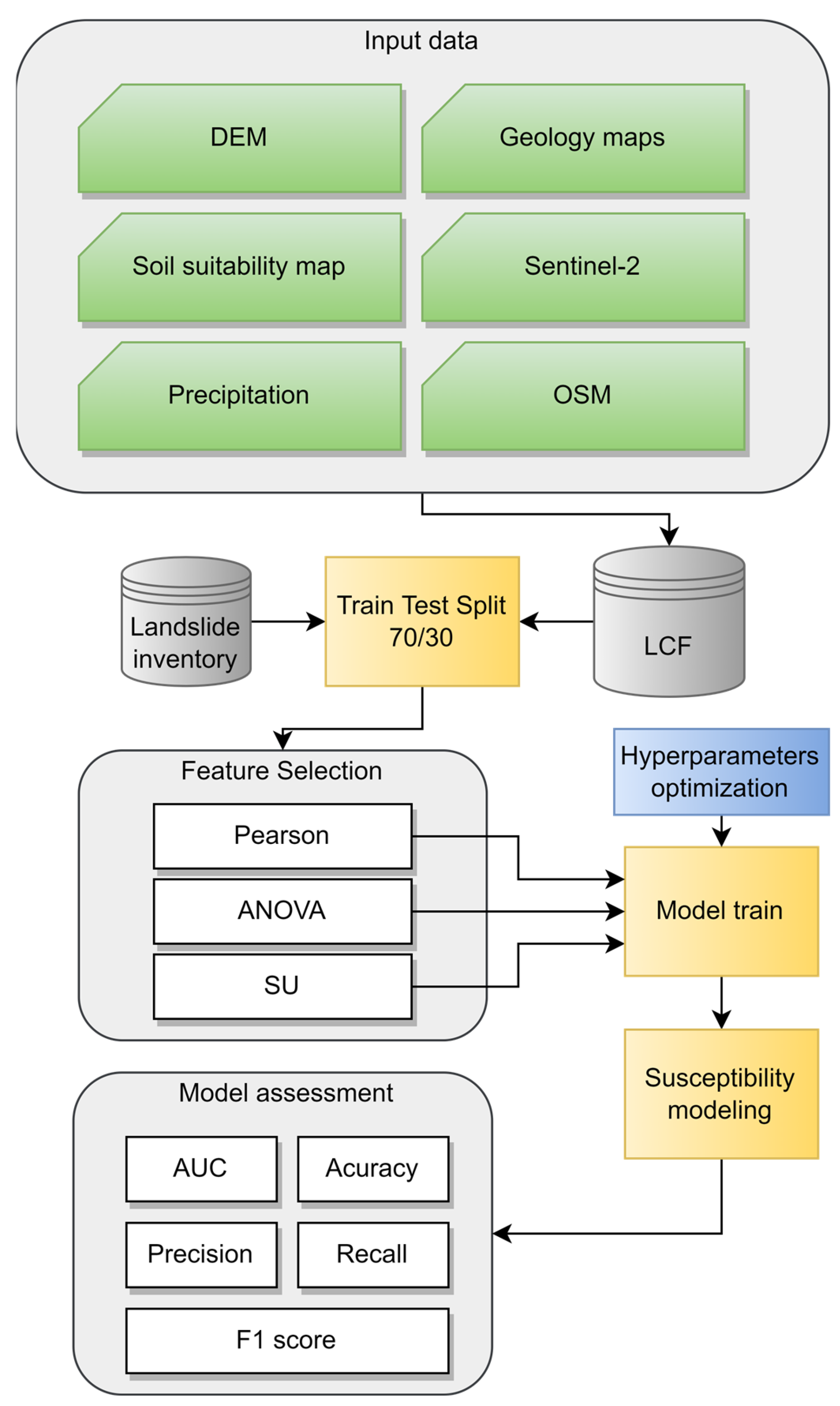
Figure 2 presents the overall flowchart of the methodology adopted in this study. The first step was to collect data from various sources and then produce LCFs, as described in Section 2.3.1. After the generation of 23 input LCFs, feature selection was performed using three methods, the Pearson correlation coefficient (PCC), analysis of variance (ANOVA), and symmetrical uncertainty (SU), as described in Section 2.3.2. To evaluate the effects of the feature selection method, model training was performed for three separate input datasets designated via the feature selection methods, as described in Section 3.3. Pixels for each selected dataset were randomly split into train and test sets with proportions of 70% and 30%, respectively, using the scikit-learn library version 1.6.1. For these three input datasets, three landslide susceptibility models were trained for each feature selection method. The next step was to optimize the XGBoost hyperparameters and train the model on the optimized parameters described in Section 2.3.3. An accuracy assessment of each susceptibility map was performed using various accuracy measures, as presented in Section 2.3.4. Input data processing, as well as the preparation of LCFs, was carried out in the ArcMap software version 10.8.1, while the Python programming language version 3.12.1 using the scikit-learn library version 1.6.1 was utilized for feature selection, susceptibility modeling, and accuracy assessment.

2.3.1. Generation of Landslide Conditioning Factors

In this study, LSM was performed based on LCFs derived from a previously presented input dataset (Section 2.2). Table 2 presents a list of the used LCFs, their sources, and application examples for susceptibility mapping found in the literature. A graphical representation of some of these factors is presented in Appendix A.1 for the Rożnów case study and Appendix A.2 for the Biały Dunajec case study. Based on the DEM data, 11 topographical and hydrology-related factors were calculated, as listed in Table 1, numbered 2 to 12. These 11 LCFs were calculated using the ArcGIS software (version 10.8.1). Aspect identifies the direction of a slope, expressed in degrees in the range of 0° to 360°, measured clockwise [76]. Slope is the rate of the maximum change in the height value related to neighboring cells [76]. Slope values are expressed in degrees and were calculated with a Z-factor = 1 and the geodetic method. The flow direction indicates the direction in which water flows out of the cell. This factor was calculated using D8 modeling—for each cell, the flow direction is encoded according to the orientation of one of the eight surrounding cells with the steepest descent [77]. Curvature factors describe the slope curvature and allow the analysis of erosion and runoff processes [78]. Three types of curvature were calculated, namely standard, profile, and planform, which are listed in Table 2. The profile curvature is parallel to the slope and describes the acceleration of the flow. Positive values indicate that the terrain is upward concave and negative convex [78]. The planform curvature is perpendicular to the maximum slope [78]. This factor is related to the convergence of the flow. Positive values represent laterally convex surfaces and negative values represent laterally concave surfaces [78]. The standard curvature is a combination of the profile and planform curvatures [78]. The compound topographic index (CTI) is a steady-state wetness index that expresses the topographical effects on hydrological processes [79]. The CTI is defined as
C T I = l n A s t a n β
where A s represents the area value, expressed as (flow direction + 1) × (pixel area in m2), and β is the slope angle. The integrated moisture index (IMI), developed in [80], describes the rate of moisture related to specific processes [81]. The IMI can be expressed as
I M I = h i l l s h a d e × 0.5 + c u r v a t u r e × 0.15 + F l o w   a c c u m u l a t i o n × 0.35
The site exposure index (SEI) is defined by the equation below and was introduced in [82]:
S E I = β × c o s π a s p e c t 180 ° 180 °
The SEI, CTI, and IMI were calculated using the Geomorphometry & Gradient Metrics Toolbox [83]. Although the SEI is not yet a widely used variable in landslide susceptibility studies, it can be easily derived from standard topographic parameters—the slope angle and terrain aspect. Its inclusion in this study was motivated by the hypothesis that slope exposure may influence moisture dynamics and thermal stress, both of which are relevant to slope instability. For instance, south- and southwest-facing slopes, which typically receive more solar radiation, may experience enhanced drying, temperature fluctuations, and vegetation stress, all of which can reduce slope cohesion and increase landslide susceptibility. While less common in the current literature, the relevance of exposure-related factors to slope stability has been documented in various geomorphological and geotechnical studies (e.g., [60]), and the SEI offers a simple, interpretable proxy to explore this relationship further in data-driven models.
The TPI is a parameter that compares the elevation of each cell in the DEM to the mean elevation of a specified neighboring cell [33]. In this study, the neighborhood was set as a rectangle of 3 × 3 pixels. The TPI was calculated using the Topography Toolbox [84]. Because of the sparsity of the OSM and river network, stream proximity was calculated based on the flow accumulation raster. With a threshold of 10,000, the flow accumulation raster was reclassified, where values above the threshold indicated water streams. The reclassified raster was converted to polyline, and proximity was calculated using the Euclidean distance method. The precipitation raster was obtained using the inverted distance weight interpolation method, with the default parameters of the neighborhood for the 11 precipitation stations. Tectonics, fault proximity, and thrust proximity were obtained by the manual vectorization of geological maps provided by the PGI and the Euclidean distance tool of ArcGIS. OSM data were also used to determine the road proximity and river proximity factors. Similarly to geologically related LCFs, soil suitability, soil texture, and soil type were acquired by the manual vectorization of soil suitability maps from the MIIP and the conversion of shape objects into raster format, and the normalized difference vegetation index (NDVI) and land cover factors were calculated based on the Sentinel-2 imagery. A land cover map was produced using supervised maximum likelihood classification based on all spectral bands of the Sentinel-2 data and the NDVI. Five land cover types were classified: water, agriculture, bare land, forest, and urban areas. The overall accuracy of this land cover map was found to be 89%.
Table 2. Landslide conditioning factors used in the presented study, together with the source data used for its generation.
LCFMethodDataData SourceApplication Example
1.DEM-DEMISOK data, https://www.geoportal.gov.pl (accessed on 8 August 2025)[35,85]
2.AspectArcGIS[41,86,87]
3.SlopeArcGIS[86,88]
4.Flow directionArGIS[12,75]
5.CurvatureArcGIS[3,41]
6.Plan curvatureArcGIS[10,86]
7.Profile curvatureArcGIS[86,87]
8.CTIArcGIS—Geomorphometry and Gradient Metrics[10,12]
9.IMIArcGIS—Geomorphometry and Gradient Metrics[12,89]
10.TPIArcGIS—Topography Toolbox[33,34]
11.SEIArcGIS—Geomorphometry and Gradient Metrics[12,75]
12.Stream proximityEuclidean distance[10,90]
13.PrecipitationIDW interpolationPrecipitation pointsIMGW data
https://danepubliczne.imgw.pl (accessed on 8 August 2025)
[13,35,91]
14.TectonicsVectorizationGeology mapsPGI data
https://geolog.pgi.gov.pl (accessed on 8 August 2025)
[13,88]
15.Fault proximityEuclidean distance[92,93]
16.Thrust proximityEuclidean distance[12,64,94]
17.Roads proximityEuclidean distanceRoad networkOSM data[95,96]
18.River proximityEuclidean distanceRiver network[13,88]
19.Soil suitabilityVectorizationSoil suitability mapsMIIP data
https://miip.geomalopolska.pl (accessed on 8 August 2025)
[12,95]
20.Soil textureVectorization[12]
21.Soil typeVectorization[35,82]
22.NDVI N I R R E D N I R + R E D ,
NIR is near-infrared band and red is red band
Satellite imageSentinel-2[33,93]
23.Land coverSupervised classificationSentinel-2[12,35]

2.3.2. Feature Selection Methods

As mentioned in the Introduction, feature selection is a crucial step in ML modeling [33]. Reducing the number of input variables is preferable, because it can reduce the model training time and improve its performance by removing features with limited predictive abilities [54,93]. In this study, three feature selection methods were used—the PCC, ANOVA, and SU. Based on the obtained PCC, F-score, and SU measures, all values were normalized to enable a direct comparison across methods and an importance evaluation (Section 3.2). Features were then ranked accordingly, and those deemed the least important were removed from further analysis. To support the elimination process, the normalized importance values were used. Normalized PCC/F-score/SU values were classified into six groups using the natural breaks (Jenks) algorithm. Features falling into the group with the lowest values were considered the least informative and were excluded from subsequent modeling. This selection step ensured that the selected features contributed meaningful information to LSM.
  • Pearson correlation
The first step in the feature selection process was to assess redundancy and correlations within the LCFs, as well as for each LCF and landslide layer. This is particularly important in LSM, where highly correlated input variables may introduce multicollinearity and reduce model transparency and the generalization ability. To address this issue, we employed the PCC, a widely used metric in quantifying the strength and direction of the linear relationship between two variables. The PCC returns values between –1 and 1, where
  • 1 indicates a perfect positive correlation;
  • 0 indicates no linear relationship;
  • −1 indicates a perfect negative correlation.
The PCC ( ρ X ,   Y ) between two variables X and Y is defined as
ρ X ,   Y = c o v ( X ,   Y ) σ X σ Y
where c o v ( X ,   Y ) is the covariance between X and Y, and σ X , σ Y are the standard deviations of each variable [97]. Since we were interested in the strength rather than the direction of the relationship, we used the absolute value of the PCC.
In our study, two types of correlation were analyzed: (1) inter-feature correlation—to identify redundancy among input variables—and (2) feature-to-target correlation—to assess the relevance of each factor with respect to landslide occurrence. Since the PCC-based selection method focused on choosing variables that were highly correlated with the target variable, it did not fully eliminate the possibility of inter-feature correlation. Some degree of redundancy may still have persisted among the selected variables, as the selection process prioritized individual predictive power over strict mutual independence.
  • ANOVA
Analysis of variance (ANOVA), originally developed in [98], is a statistical method used to assess how one or more independent variables influence a dependent variable [99]. It does so by comparing the variance between group means to the variance within these groups. The core idea of ANOVA is to test whether the means of different groups are statistically significantly different from one another.
The null hypothesis (H0) assumes that all group means are equal, whereas the alternative hypothesis (H1) posits that at least one group mean differs. The outcome of this test is the F-statistic (F-score), which determines whether to reject or retain the null hypothesis.
To compute the F-score, ANOVA uses the following components:
  • Grand mean (GM): the average of all observations across all groups;
  • Sum of squares (SS): is the sum of the squared deviations of data points from a specific mean, measuring the variability of the data around that mean.
  • Mean squares (MS): This is calculated as the ratio of the corresponding sum of squares to their degrees of freedom (df):
M S b e t w e e n = S S b e t w e e n d f b e t w e e n ,   M S w i t h i n = S S w i t h i n d f w i t h i n
where:
  • SSbetween is the sum of squared differences between each group mean and the grand mean, weighted by the group size.
  • SSwithin is the sum of squared differences between individual observations and their respective group means.
The F-score is then defined as [99]
F = M S b e t w e e n   g r o u p s M S w i t h i n   g r o u p s
where
  • M S b e t w e e n   g r o u p s represents the average variability between groups (e.g., landslide vs. non-landslide), measuring how much the group means differ from the grand mean;
  • M S w i t h i n   g r o u p s reflects the average variability within each group, indicating the internal dispersion of values around each group’s mean.
A higher F-score suggests that the variance between groups is significantly larger than the variance within groups, indicating that the feature effectively discriminates between classes and is potentially valuable for classification. Conversely, a low F-score implies that the feature does not differ much across groups and may be less useful.
This metric is especially useful in ranking input variables based on their statistical relevance to the target variable before model training.
  • Symmetrical Uncertainty (SU)
SU is a measure that allows the analysis of the relevance and redundancy between two variables. It is defined as
S U = H X + H Y H X , Y H X + H Y
where H X and H Y are the Shannon entropies of variables X and Y .   H X , Y describes the joint entropies of the variables. SU values are between 0 and 1, where 1 means that the variables are completely dependent and 0 means that the variables are independent [33].

2.3.3. Landslide Susceptibility Mapping Using XGBoost

XGBoost is an ML algorithm based on multiple decision trees and gradient boosting, developed by Tianqi Chen and Carlos Guestrin [100]. In XGBoost (version 2.1.2), the output is predicted by a tree ensemble model, which can be expressed by the following equation:
y ^ i = ϕ x i = k = 1 K f k x i ,       f k F
where F describes the space of CART, x i is a feature value, and f k is the tree structure at step k. The training set of trees has to minimize the following objective function:
L ϕ = i l ( y ^ i ,   y i ) + k Ω ( f k )
where l is a loss function that measures the difference between predicted values y ^ i and target values y i . Ω is a penalty component to control model complexity, defined as
Ω f = γ T + 1 2 λ w 2
where γ ,   λ are regularization parameters that prevent overfitting, T is the number of leaves in the tree, and w is the score of each leaf in the tree. To evaluate split candidates while constructing the tree, the following formula is used:
G =   1 2 G L E F T 2 H L E F T + λ + G R I G H T 2 H R I G H T + λ G L E F T + G R I G H T 2 H L E F T + H R I G H T + λ γ
where G L E F T 2 H L E F T + λ is the similarity score of the left node, and G R I G H T 2 H R I G H T + λ is that of the right node. G L E F T + G R I G H T 2 H L E F T + H R I G H T + λ is the similarity score of the root node. If the value of G is greater than 0, the algorithm performs the split [36].
XGBoost is a highly efficient and accurate algorithm, but it has many hyperparameters that need to be optimized to achieve good performance. For instance, in the case of landslide and non-landslide classes, the significant issue of imbalanced data may arise. To address this, we utilized the scale_pos_weight parameter to deal with imbalanced data. In total, we optimized several hyperparameters, including num_boost_round, learning_rate, max_depth, gamma, max_delta_step, min_child_weight, subsample, colsample_bytree, and scale_pos_weight. These hyperparameters were separately optimized for each train–test combination to achieve the best results. In this study, optimization was performed using the Bayesian optimization algorithm [101], which is often utilized in LSM [36].
Because the XGBoost model returns probabilities of landslide occurrence in every pixel, a decision has to be made regarding where to set a threshold that separates non-landslide pixels from landslide pixels. One solution described in various papers [33,34] classifies probability values into five categorical classes—very low, low, medium, high, and very high—and it is assumed that high and very high pixels represent landslide occurrences. This allows for the calculation of the widely used in classification accuracy measure. Various classification methods are utilized in the literature for susceptibility class generation, including quantile–quantile [10,13,102], natural breaks [10,20,102], equal intervals [20,102], and the standard deviation [10,102]. In this study, we classified the probability maps into categorical susceptibility classes using all five methods; however, based on the visual interpretation of the susceptibility maps and analysis of the histograms, natural breaks produced the best results. Moreover, natural breaks classification is widely used in geospatial analysis for thematic mapping, as it minimizes the within-class variance and maximizes the between-class variance. It is particularly suitable for skewed or non-uniform distributions of susceptibility values and ensures that the classification better reflects the natural grouping of the data [103]. Pixels classified into the “high” and “very high” susceptibility classes were interpreted as landslide-prone areas for the purpose of producing binary evaluation metrics (Section 2.3.4).

2.3.4. Accuracy Assessment

An important step in developing a model for landslide prediction is the accuracy assessment of the model. One of the most widely used methods of ML model evaluation is the analysis of a confusion matrix and its deliverables. Widely used measures include the overall accuracy (OA), precision, recall, and F1-score, which are defined as follows:
O A = T P + T N T P + F P + T N + F N
P r e c i s i o n = T P T P + F P
R e c a l l = T P T P + F N
F 1 = 2 · P r e c i s i o n × R e c a l l P r e c i s i o n + R e c a l l
where T P represents true positive pixels, T N true negative pixels, F P false positive pixels, and F N false negative pixels.
In addition to these four measures, a common choice among researchers is the area under the receiver operating characteristic curve (AUROC), also known as the area under the curve (AUC). The AUC measures how the model tests various thresholds for true and false pixels [104]. The AUC values range from 0 to 1, where 1 indicates perfect predictions. Since the previously mentioned measures are threshold-dependent, the AUC was also utilized to quantitatively evaluate the performance of the LSM developed for the Biały Dunajec and Rożnów Lake case studies.

3. Results

3.1. Feature Correlation

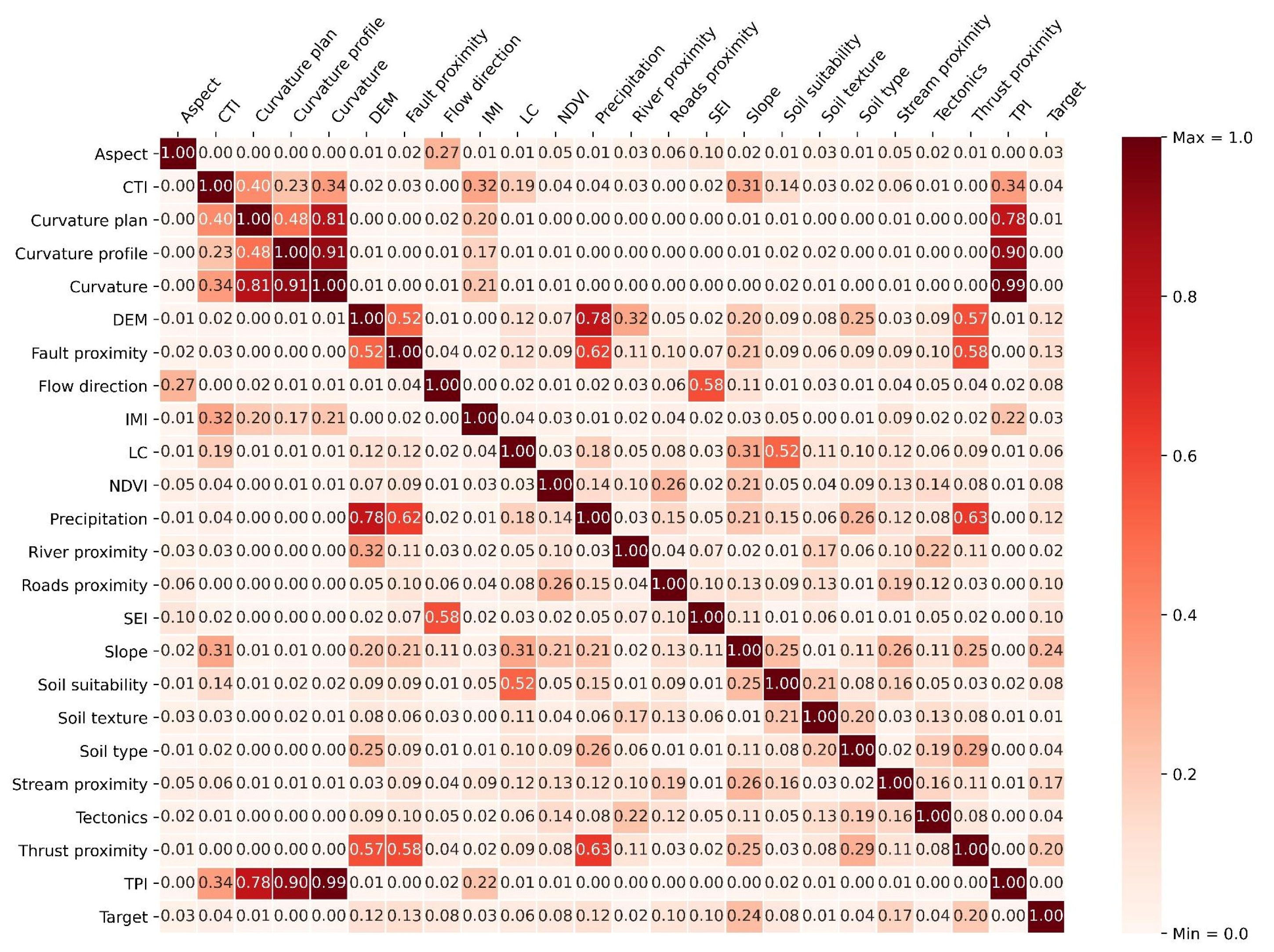
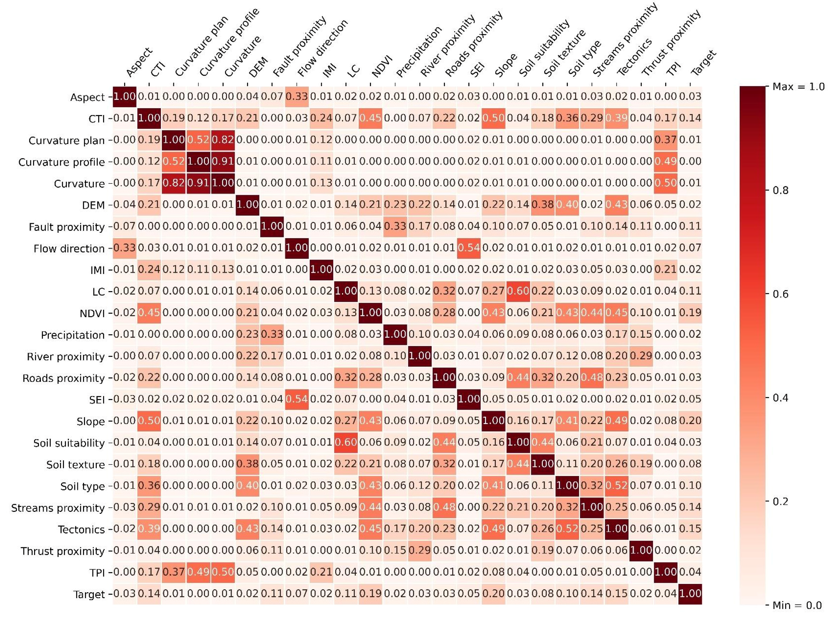
Figure 3 shows the PCC matrix for the Biały Dunajec case study, and Figure 4 shows the PCC matrix for the Rożnów case study. For the PCC, to increase the readability, we used its absolute value to rank variables according to the strength of their linear associations, irrespective of the direction.
As can be noted, the TPI is highly correlated with the curvature, planar curvature, and profile curvature, which are also correlated with each other. In addition, these variables were not correlated with the target dataset (landslides). This implies that these features are likely to be useless for LSM. The highest correlation with the target layer is represented by the slope variable (0.24). In addition, the landslide variable is somewhat correlated with the thrust proximity (0.20), DEM (0.12), fault proximity (0.13), stream proximity (0.17), and precipitation (0.12) variables. In contrast, the layers that are not correlated with the target layers are the TPI (0.00), profile curvature (0.00), planar curvature (0.01), and curvature (0.00).
Figure 4 represents the PCC matrix for the Rożnów case study area. Similarly to the Biały Dunajec case study, the TPI variable is also highly correlated with the curvature, planar curvature, and profile curvature. In this case, the highest correlation with the target dataset is also represented by the slope feature (0.20). However, in the Rożnów case study, a different set of moderately correlated features was observed: NDVI, tectonics, and CTI, with correlation values of 0.19, 0.15, and 0.14, respectively. In contrast, these variables exhibited lower correlation values in the Biały Dunajec area. Variables showing no significant correlation with the target layer remained consistent across both study areas and included the profile curvature (0.00), planform curvature (0.01), and general curvature (0.01).

3.2. Feature Importance Analysis

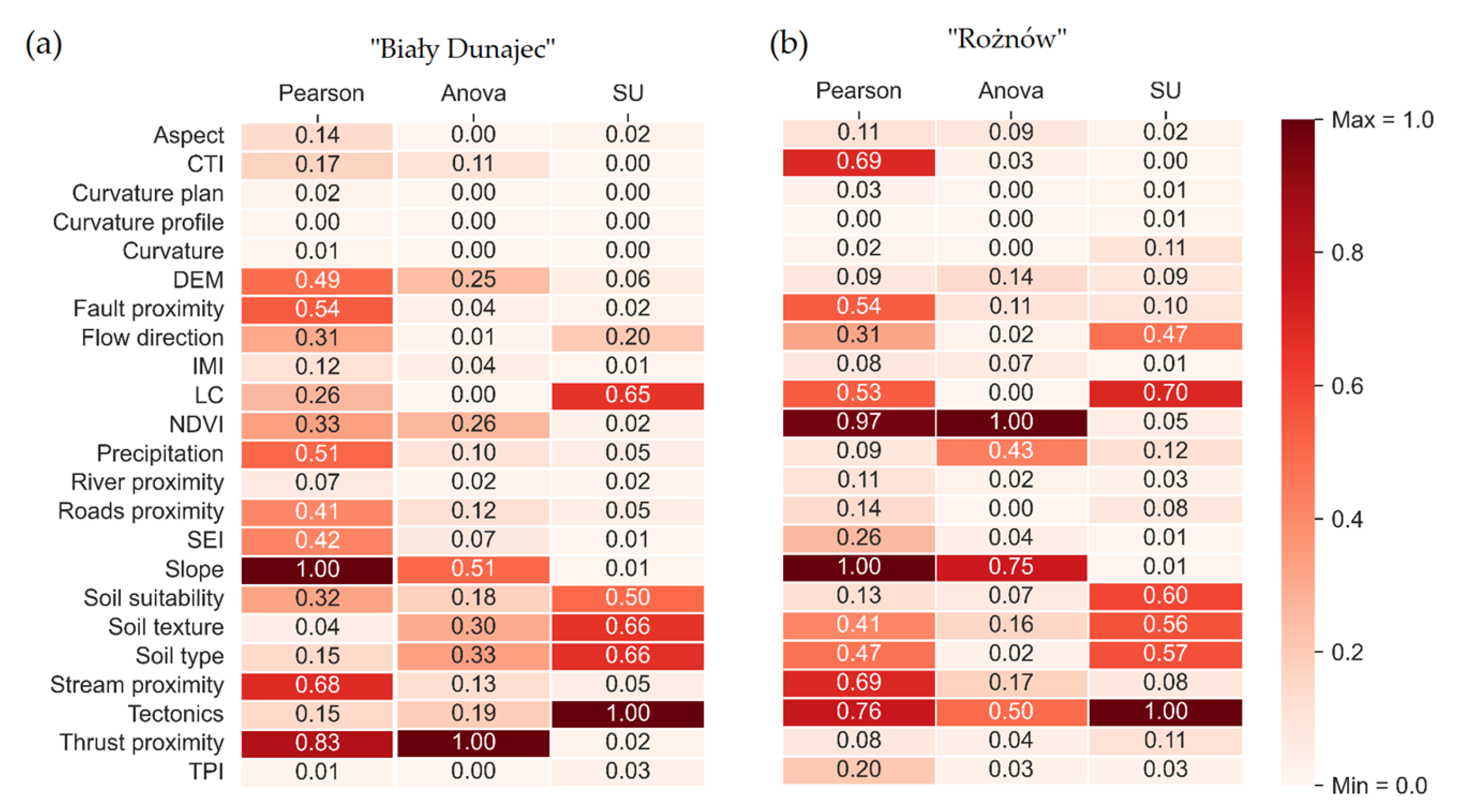
Figure 5a,b present the results of the feature importance analysis using the three feature selection methods. The importance scores were normalized to allow comparisons between methods. For the Biały Dunajec case study (Figure 5), the slope is most important, followed by thrust proximity and stream proximity, for the PCC method. However, the ANOVA method demonstrated the thrust proximity to be the most important, followed by the slope. The results for the SU method indicate that categorical features are the most important. This may be due to the limited number of categories within the data, which reduces the variability and weakens the correlation signal. Among the non-categorical variables, the flow direction proved to be the most important feature for the SU model. The results for the most important features were different between the ANOVA and SU. Nevertheless, for each feature selection method, the curvature-related features were the most insignificant.
The results for the Rożnów Lake dataset differ from those for Biały Dunajec. For the PCC method, slope was identified as the most important feature, followed by the NDVI, which was less influential in the case of the Biały Dunajec study area. In addition, the ANOVA scored the NDVI and slope as the most important features. However, the scores in SU feature importance for Rożnów are similar to those for Biały Dunajec. As previously mentioned, the elevation differs between the two study areas, and, as shown in Figure 5, the DEM proved to be a more important feature in the Biały Dunajec case study, according to both the PCC and ANOVA feature selection methods.

3.3. Various Strategies of LSM—Selected Features

As mentioned in the Methodology section, the natural breaks method was used to group features according to their similarity and to remove features that fell into the group with the lowest importance values. Finally, for the two study cases, six strategies of input features were tested. Table 3 summarizes the features that were preserved and the features that were rejected from further analysis in all six modeling strategies.
As shown in Table 3, for both study areas, the curvature layers were identified as unsuitable LCFs when using the PCC and ANOVA feature selection methods. In contrast, the SU method excluded the CTI, IMI, and river proximity, indicating that these features were not relevant for modeling in either case. Consequently, they were not included in the subsequent LSM process.

3.4. Landslide Susceptibility Maps and Accuracy Measures

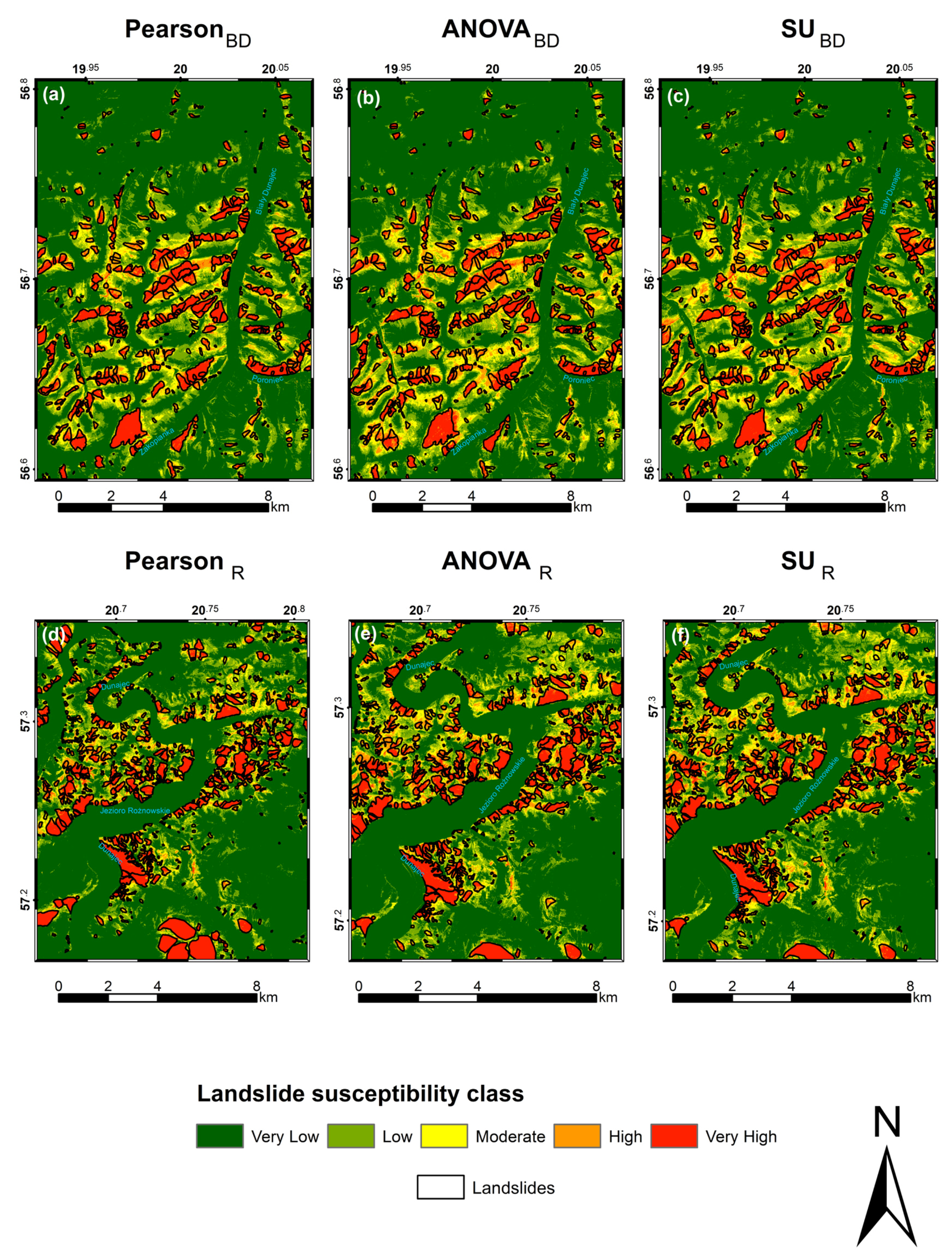
The landslide susceptibility maps are shown in Figure 6. Visual inspection does not reveal any substantial differences between the maps, as they appear nearly identical. It is only through accuracy indices that slight variations become noticeable. Therefore, the accuracy measures are presented in Table 4 and AUC charts are presented in Figure 7.
Based on Table 4, all models achieve high OA (0.90 to 0.93) and recall (0.89 to 0.94), indicating strong performance in identifying actual landslide areas. However, the precision is consistently lower (0.57 to 0.69), suggesting the overprediction of landslide-prone areas. This trade-off is generally acceptable in risk management, as it minimizes the chance of missing actual landslides. Models using the SU feature selection method show slightly weaker performance, especially in the Biały Dunajec case, with the lowest precision (0.57) and F1-score (0.69). In contrast, the PCC and ANOVA methods yield more balanced results.
All models demonstrated strong discriminative abilities, with the AUC values exceeding 0.97 (Figure 7), confirming their robustness for LSM. In the Biały Dunajec case study, the AUC scores were 0.985 (PCC), 0.981 (ANOVA), and 0.981 (SU), indicating excellent model performance with minimal variation between feature selection methods. In comparison, the models for the Rożnów case study achieved slightly lower AUC values: 0.983 (PCC), 0.972 (ANOVA), and 0.980 (SU). Among them, the ANOVA-based model in Rożnów showed the lowest AUC, suggesting a somewhat reduced ability to capture landslide patterns in this area.
While the differences between models were small (maximum ΔAUC = 0.013), the Biały Dunajec models performed marginally better, possibly due to geomorphological differences or data quality variations. As shown in Table 4, although SU performed comparably in terms of the AUC, it generally produced the lowest values across all metrics, particularly in Biały Dunajec.
The relatively small performance differences between the feature selection methods may be due to the high number of input LCFs used in modeling. Initially, 23 LCFs were prepared, and, after feature selection, 20 (Rożnów) and 17 (Biały Dunajec) were retained in the PCC-based selection, which consistently yielded the best results. This suggests that the most effective approach may involve selecting features highly correlated with landslide occurrence.
However, it is important to note that the AUC reflects only the discriminative ability and does not capture spatial accuracy or practical usability. Therefore, it should be interpreted alongside other performance measures.

4. Discussion

4.1. Correlations Between LCFs

The PCC analysis revealed redundancy among several LCFs, particularly the curvature, planar curvature, profile curvature, and TPI, which showed strong mutual correlations in both study areas. As they described similar terrain morphologies and had weak correlations with landslide occurrence, they were excluded from further modeling. In contrast, slope showed the strongest and most consistent correlations with the target variable. Beyond these anticipated relationships, several unexpected correlations emerged, warranting further discussion. In Biały Dunajec, a strong correlation was observed between precipitation and DEM, which aligns with prior studies indicating increased precipitation with altitude [105,106]. This pattern was less pronounced in the Rożnów region, likely due to its lower overall elevation and smaller altitudinal range.
More surprisingly, a notable correlation was also found between precipitation and fault proximity, as well as between DEM and fault proximity. These associations may reflect the influence of mountainous, tectonically active zones, where higher-elevation areas often coincide with major fault systems and receive greater orographic precipitation. The fault proximity may therefore indirectly encapsulate both topographic and climatic gradients in such regions.
Another interesting correlation was observed between soil suitability and land cover. This relationship can be explained by the dependence of the vegetation type and density on the soil fertility, structure, and moisture retention capacity—all of which are captured in soil suitability indices. In turn, vegetation cover influences NDVI values and surface hydrological processes, indirectly affecting landslide susceptibility.
Similarly, correlations between thrust proximity and precipitation may stem from regional-scale geological and climatic interactions. Thrust zones are often associated with elevated, folded terrain, which tends to receive more rainfall due to orographic effects. These correlations, while not indicating direct causality, highlight the complex interplay between geomorphological, geological, and climatic factors within mountainous landscapes.
Overall, these findings demonstrate that not all correlations within susceptibility modeling are immediately intuitive. Some reflect underlying geomorphic or tectonic structures, while others result from broader landscape processes. Interpreting such relationships carefully is essential to ensure that variable selection in LSM is both statistically and physically meaningful.

4.2. Feature Selection

Each feature selection method resulted in different importance scores for the analyzed variables. In addition, the results of the same method varied for different areas. The PCC approach to feature selection rejected six features for Biały Dunajec and three for Rożnów. However, the features rejected in the Rożnów case study were also listed among the rejected variables in the Biały Dunajec case study, namely the curvature, planar curvature, and profile curvature. The ANOVA method rejected most features. More specifically, nine variables were rejected for Biały Dunajec and six for the Rożnów case study. Similarly to the PCC method, the ANOVA also rejected curvature-related variables for both areas. Interestingly, the ANOVA method rejected the DEM variable in the Rożnów dataset. The PCC method also indicated a low correlation between the DEM and landslide layer. The reason for the DEM’s rejection might be because there are 11 LCFs that are derivatives of DEM features, which can present stronger relationships with landslide occurrence (e.g., slope). Another difference between the ANOVA scores for each area is that the feature with the highest score in the Biały Dunajec case is the thrust proximity, which received a very low score in the Rożnów case. Conversely, the feature with the highest ANOVA score in Rożnów is the CTI, which had low importance in the Biały Dunajec dataset. These differences show that LCFs have various degrees of importance for LSM in a given area. However, the SU method yielded similar results for both study cases in terms of highly important variables. Nonetheless, when using this method, we rejected considerably more features in Biały Dunajec than in the Rożnów case study. The rejected features in Rożnów, namely the CTI, IMI, and river proximity, were likewise among those rejected in the Biały Dunajec case study.

4.3. Accuracy Assessment of Various Models

When comparing the AUC values, the models trained on the Biały Dunajec and Rożnów datasets achieved comparable results, with only minor differences observed across feature selection methods. These small variations in performance may stem from differences in area size and data characteristics. The Rożnów case study covered an area that was 7 km2 smaller than in Biały Dunajec, which likely resulted in fewer training samples. However, the landslide area was 1.2 km2 larger in Rożnów, potentially providing more relevant positive samples.
The lowest performance for the Biały Dunajec models was observed with the SU feature set. This may be due to SU’s preference for categorical features, which could lead to the exclusion of more informative non-categorical variables such as thrust proximity or DEM—features whose importance scores were high in other selection methods. Interestingly, the SU-based model performed relatively well on the Rożnów dataset, possibly due to lower variability in this area (e.g., elevation differences reach up to 539 m in Biały Dunajec but only 381 m in Rożnów).
Models using the PCC and ANOVA-based feature sets yielded similarly strong results for the Biały Dunajec area. For the Rożnów area, PCC-based models showed slightly better performance, with the precision, recall, and F1-scores being higher by approximately 3%, 1%, and 2%, respectively, compared to their Biały Dunajec counterparts. Although the PCC and ANOVA methods reduced the input feature set by six and nine features, respectively, their overall performance remained comparable. However, models based on PCC-selected features were more computationally intensive.
Overall, when considering various accuracy metrics and the number of removed variables, no significant changes in the accuracy of the LSM were observed. This may be due to the high number of input variables used in the modeling process, where the information contained in the removed variables was likely preserved within the remaining ones.

4.4. Comparison with Other Related Studies

The results obtained in this study confirm the high effectiveness of the XGBoost algorithm in LSM, which is consistent with numerous previous studies [33,36,48,63]. As shown in Table 5, the AUC values reported in the literature varied between 0.74 and 0.96 depending on the study area, dataset characteristics, and methodological approach. In comparison, the AUC values obtained in this work (0.985 for Biały Dunajec and 0.983 for Rożnów) are among the highest, indicating excellent model performance and generalization abilities.
The authors of [33] achieved an AUC of 0.957, while the authors of [63] reported an AUC of 0.96, both using extensive feature sets and favorable training–testing splits (70–30% and 80–20%, respectively). Our models performed slightly better in terms of the AUC, which may have resulted from the high number of input variables, parameter tuning, and train–test split ratio. Conversely, the authors of [48] reported the lowest AUC of 0.74, likely due to testing their model on an entirely separate area, emphasizing the difficulty in model transferability across different terrains. Similar results were demonstrated in [12].
In terms of the F1-score, the results presented here (up to 0.79 for PCC) are superior to those reported in [48] (0.65) and [36] but comparable to those reported in [63] (0.88). Our models also achieved consistently high recall (up to 0.94), which is crucial in minimizing false negatives in landslide predictions. However, as also observed by other authors, the precision scores in our case were lower (e.g., 0.57–0.69), suggesting that the model tended to overpredict landslides. A similar trend was reported by the authors of [48], who observed relatively low precision of 0.6 in LSM. This imbalance between recall and precision can be attributed to multiple factors, including class imbalance, terrain complexity, and the nature of the selected features. Importantly, while lower precision may result in the overidentification of landslide-prone areas, it is generally preferable from a hazard management perspective, as it reduces the risk of overlooking true landslide locations.
Differences in the number and type of LCFs, the feature selection techniques, and the geographic characteristics of the study areas explain most of the variation between the presented results. For instance, the SU and ANOVA feature selection methods resulted in marginally lower precision compared to the PCC method, which is consistent with trade-offs commonly reported in the literature. Furthermore, some previous studies did not report all classification metrics (e.g., [33]), which limits the capacity for direct comparisons. Overall, the performance of the XGBoost-based models developed in this study was consistent with that of those previously reported. This confirms the robustness of the algorithm and highlights the importance of adapting the model parameters and features to the characteristics of the local environment.
Moreover, incorporating multi-source information could aid LSM, particularly by integrating more specific or dynamic variables such as rainfall anomalies or the daily rainfall intensity, which may better capture triggering conditions than long-term averages. Similarly, including more detailed geological maps—where available—could enhance the spatial resolution of lithological information.
However, we do not necessarily believe that increasing the spatial resolution of the DEM will lead to better model performance. Several recent studies have shown that higher-resolution DEMs do not consistently improve susceptibility outcomes and may even introduce noise or overfitting in some ML frameworks, particularly in heterogeneous terrain [75,107]. The same applies to DEM-derived factors such as curvature or the TPI, which may become unstable at very fine scales. Accordingly, in our future work, we will focus on integrating heterogeneous data with physically based models and constraints, aiming to enhance the interpretability and generalizability of LSM.

4.5. Potential Applicability and Future Perspectives of Feature Selection Methods in Diverse Geological Settings

Although the three feature selection methods evaluated in this study yielded comparable results in terms of overall model performance, their applicability across different geological settings remains uncertain. Each method emphasizes different aspects of predictor relevance: the PCC identifies linear correlations, ANOVA focuses on statistical separability, and SU captures non-linear and categorical relationships. As such, the effectiveness of each method is inherently dependent on the nature and structure of the input data, which are strongly influenced by the geological context.
In homogeneous flysch terrains, as in our study areas in the Carpathians, multiple geomorphometric variables tend to co-vary. However, in more heterogeneous regions—such as crystalline massifs (e.g., the Sudetes) or tectonically complex zones (e.g., the Alps)—LCFs may exhibit non-linear interactions and greater lithological diversity, potentially diminishing the utility of correlation-based methods such as the PCC. In such cases, information-theoretic approaches (e.g., SU) may perform better in capturing the influence of categorical variables such as the rock type or fault proximity.
Moreover, topography-driven predictors, which were the most influential in this study, may be less dominant in flatter or sedimentary environments, where other variables (e.g., land use, soil properties, hydrological factors) may play a larger role. This underscores the need for context-specific feature selection strategies, tailored to the prevailing geological and geomorphological conditions.
Therefore, while the current findings demonstrate that different feature selection methods can produce robust LSM results within a relatively uniform geological framework, their transferability and reliability across geologically diverse settings remain limited. To better understand these limitations, future research should focus on systematically comparing feature selection techniques in contrasting geological environments and evaluating how they interact with specific terrain, lithology, and climate conditions. This would provide valuable insights into the generalizability of LSM methodologies and support the development of adaptive, geology-aware feature selection frameworks.

4.6. Beyond Accuracy Measures: A Funcional Perspective on LSM Validity Assessment—Metrics, Challenges, and Temporal Relevance

While the AUC and other accuracy measures area commonly used, it primarily reflects a model’s ability to reproduce known landslide occurrences. High AUC values—especially those approaching 1—indicate a high TPR and low FPR across all thresholds. However, such values mostly capture the retrospective accuracy of the model in identifying past landslide locations, rather than its ability to generalize or predict future hazardous zones.
The true value of a landslide susceptibility model lies not only in its capacity to recreate the spatial distribution of historical landslides but, more importantly, in its ability to highlight new, potentially unstable areas. From this perspective, models with extremely high AUC values may not always provide the most meaningful outputs for risk assessment or planning. In some cases, high AUC values can result from overfitting, particularly when the study area is spatially limited and exhibits low variability in terms of LCFs.
As shown in Table 5, the AUC is the most frequently used metric in susceptibility modeling. However, several studies—including the present one—also report threshold-dependent metrics such as the overall accuracy, precision, recall, and F1-score. These metrics, while informative, are inherently sensitive to the selection of classification thresholds, which are often used to distinguish landslide-prone terrain (typically assigned to high and very high susceptibility classes) from stable areas. This binarization of continuous susceptibility values may oversimplify model outputs and introduces limitations in how performance is interpreted. Moreover, the accuracy, precision, recall, and F1-score depend on the sampling strategy, the balance between positive and negative instances, and the spatial distribution of the mapped landslides. They also do not consider the geomorphological plausibility of predicted zones. For instance, a high recall value may indicate that most landslides are captured, but it does not guarantee that the predicted unstable areas are meaningful from a geomorphological standpoint. Performance metrics offer additional advantages by highlighting the proportion of the study area classified as most susceptible, which can be useful for land use planning. However, they do not provide information about the spatial accuracy of the map, i.e., whether the locations identified as unstable align with the actual geomorphological conditions.
A more robust and operationally relevant evaluation strategy would involve temporal validation. In this approach, landslides triggered by a specific event (e.g., intense rainfall or seismic activity) are used to train the model, and the resulting susceptibility map is validated against landslides that occurred during a subsequent triggering event. This method provides a more realistic estimate of the predictive performance in future scenarios. Unfortunately, in this study, such validation was not feasible due to the lack of consistent temporal information in the available landslide inventory.
It is important to emphasize that statistically created LSM are functional in nature, meaning that their predictive value depends entirely on the type, quantity, quality, and spatial–temporal representativeness of the landslide and geo-environmental data used. Consequently, susceptibility maps do not have a predefined period of validity. They remain meaningful as long as the underlying relationships between landslides and conditioning factors remain stable. However, in cases where significant changes occur—such as land use modifications, climate change, or the occurrence of exceptional triggering events—these models should be reassessed and, if necessary, recalibrated, as their functional relationships may no longer hold.

5. Conclusions

The studied areas in Southern Poland are highly susceptible to landslides, highlighting the importance of continuous monitoring and reliable LSM. In this study, we applied the XGBoost algorithm with Bayesian hyperparameter optimization and evaluated three feature selection methods—the PCC, ANOVA, and SU.
Consistent with findings in the literature, ML models achieved high predictive performance, with AUC values of 0.985 and 0.980 for the Biały Dunajec and Rożnów areas, respectively. Despite the slightly higher AUC in Biały Dunajec, the overall accuracy, precision, recall, and F1-scores were comparable in both regions. Notably, the model for the Rożnów case study showed slightly higher precision (0.69 vs. 0.65) and a higher F1-score (0.79 vs. 0.77) when using PCC-selected features. All models demonstrated high recall (up to 0.94), which is critical for hazard mitigation. However, the relatively lower precision reflects a common trade-off in LSM—favoring overprediction to minimize missed landslide events.
The PCC analysis revealed redundancy among several geomorphological variables—the curvature, planar curvature, profile curvature, and TPI—which contributed little to the predictive performance. In contrast, slope emerged as the most influential factor in both areas. Differences in variable correlations, such as between elevation and precipitation, underscored the distinct topographic characteristics of the two sites. Our results confirm the robustness of XGBoost in LSM and emphasize the spatial variability of LSM. While SU tended to retain categorical features, the PCC and ANOVA preserved more topographically informative ones, such as DEM and thrust proximity. Nevertheless, XGBoost models based on each method produced similarly strong results. Importantly, we show that, even with the removal of some LCFs, the model accuracy remains stable when an extended set of LCFs is used.
Although both areas belong to the Carpathian flysch zone, their geological distinctions allowed for a meaningful evaluation of model generalizability. Nevertheless, to further assess the broader applicability of feature selection methods, future studies should test them in geologically distinct environments such as the Alps or the Sudetes. Since LCFs are region-specific, adapting the feature sets to the local conditions remains essential.
In summary, this study confirms that XGBoost, when combined with a carefully selected set of external features, is a powerful tool for LSM. In future work, we will focus on integrating heterogeneous data sources with physically based models and constraints to enhance both the interpretability and generalizability of susceptibility assessments.

Author Contributions

Conceptualization, K.P.-F.; methodology, K.P.-F.; software, T.L.; validation, T.L.; formal analysis, T.L.; investigation, T.L. and K.P.-F.; data curation, T.L.; writing—original draft preparation, K.P.-F. and T.L.; writing—review and editing, K.P.-F.; visualization, K.P.-F. and T.L.; supervision, K.P.-F.; project administration, K.P.-F.; funding acquisition, K.P.-F. All authors have read and agreed to the published version of the manuscript.

Funding

This research was funded by internal resources from the Institute of Geodesy and Geoinformatics (research subsidy) of University of Environmental and Life Sciences in Wroclaw.

Institutional Review Board Statement

Not applicable.

Informed Consent Statement

Not applicable.

Data Availability Statement

The raw data supporting the conclusions of this article will be made available by the authors on request.

Acknowledgments

During the preparation of this manuscript, the authors used Paperpal version 5.8.0 for the purposes of text editing. The authors have reviewed and edited the output and take full responsibility for the content of this publication.

Conflicts of Interest

The authors declare no conflicts of interest.

Appendix A

A graphical representation of the landslide conditioning factors is presented in Appendix A.1 for the Biały Dunajec study case and in Appendix A.2 for Rożnów study case.

Appendix A.1. Landslide Conditioning Factors for the Biały Dunajec Case Study
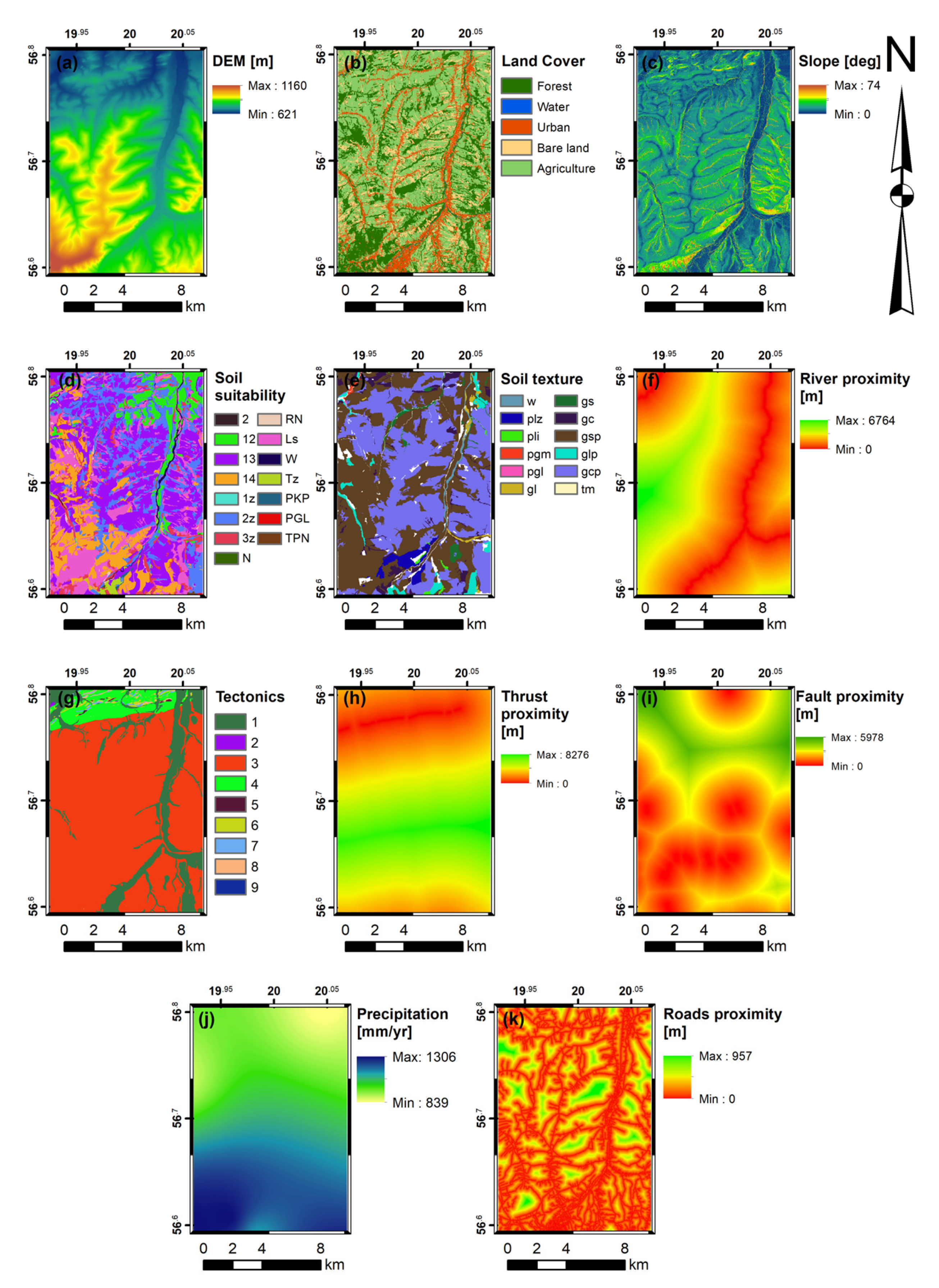
Figure A1. Example of graphical representation of landslide conditioning factors including elevation (a), land cover (b), slope (c) soil suitability (d), soil texture (e), river proximity (f), tectonics (g), thrust proximity (h), fault proximity (i), precipitation (j), roads proximity (k) for Biały Dunajec case study.
Applsci 15 08955 g0a1

Appendix A.2. Landslide Conditioning Factors for the Rożnów Case Study
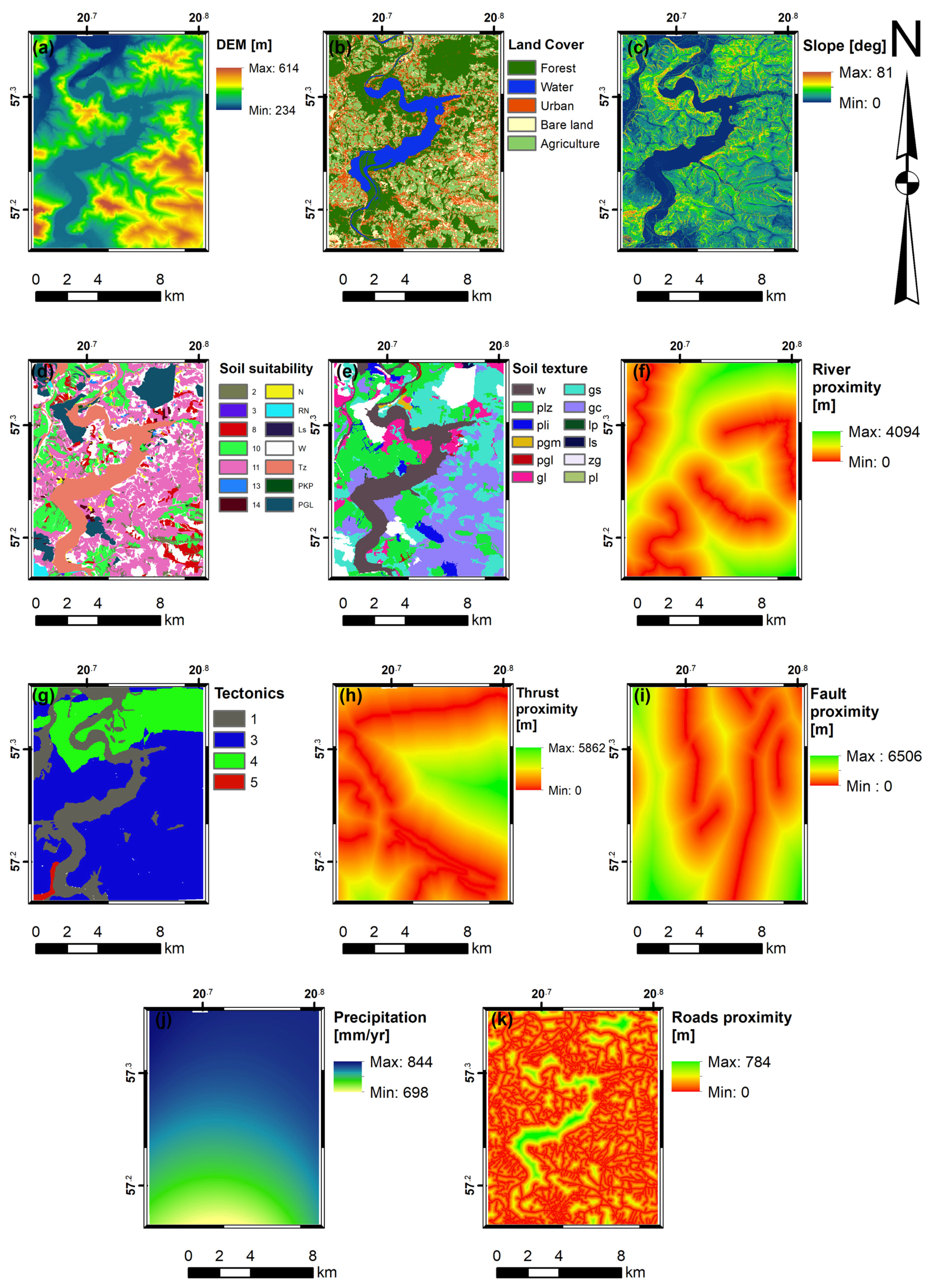
Figure A2. Example of landslide conditioning factors including elevation (a), land cover (b), slope (c) soil suitability (d), soil texture (e), river proximity (f), tectonics (g), thrust proximity (h), fault proximity (i), precipitation (j), roads proximity (k) for Rożnów case study.
Applsci 15 08955 g0a2

Appendix A.3. Description of Symbols Used for Categorical Landslide Conditioning Factors

LCFSymbolDescription
Soil suitability2good wheat
3defective wheat
8strong grain and fodder
10highland wheat
11highland grain
12weak rye
13highland oat–potato
14arable soils intended for grassland
1zvery good and good grassland
2zmedium grassland
3zweak and very weak grassland
Nwasteland
RNagriculturally unsuitable soil
Lsforests
Wwater
Tzurban areas
PKPPolish State Railway areas
PGLState Forests National Forest Holding areas
TPNTatra National Park
Soil texturewwater
plzsilt
plisilt clay
pgmstrong clay sands
pgllight clay sands
gllight clay
gsmedium clays
gcheavy clays
lpsilty loams
lsloess and loess formation
zgclay gravel
plloose sands
gspmedium silty clays
glplight silty clays
gcpheavy silty clays
tmpeat and silt
Tectonics1Quaternary
2Neogen
3Paleogene
4Upper Cretaceous
5Upper Jurassic
6malm–neakon
7Upper Jurassic
8Middle Jurassic
9Triassic

References

  1. Schuster, R.L.; Fleming, R.W. Economic losses and fatalities due to landslides. Bull. Assoc. Eng. Geol. 1986, 23, 11–28. [Google Scholar] [CrossRef]
  2. Schuster, R.L.; Highland, L.M. Socioeconomic and Environmental Impacts of Landslides in the Western Hemisphere; Open-File Report 2001-276; USGS: Reston, VA, USA, 2001. [CrossRef]
  3. Prakash, N.; Manconi, A.; Loew, S. Mapping landslides on EO data: Performance of deep learning models vs. Traditional machine learning models. Remote Sens. 2020, 2, 346. [Google Scholar] [CrossRef]
  4. Haque, U.; Blum, P.; Da Silva, P.F.; Andersen, P.; Pilz, J.; Chalov, S.R.; Malet, J.P.; Auflič, M.J.; Andres, N.; Poyiadji, E.; et al. Fatal landslides in Europe. Landslides 2016, 13, 1545–1554. [Google Scholar] [CrossRef]
  5. Froude, M.J.; Petley, D.N. Global fatal landslide occurrence from 2004 to 2016. Nat. Hazards Earth Syst. Sci. 2018, 18, 2161–2181. [Google Scholar] [CrossRef]
  6. Fidan, S.; Tanyaş, H.; Akbaş, A.; Lombardo, L.; Petley, D.N.; Görüm, T. Understanding fatal landslides at global scales: A summary of topographic, climatic, and anthropogenic perspectives. Nat. Hazards 2024, 120, 6437–6455. [Google Scholar] [CrossRef]
  7. Varnes, D.J. Landslide types and processes. In Landslides and Engineering Practice; Literary Licensing, LLC.: Whitefish, MT, USA, 1958; Volume 24, pp. 20–47. [Google Scholar]
  8. Hungr, O.; Leroueil, S.; Picarelli, L. The Varnes classification of landslide types, an update. Landslides 2014, 11, 167–194. [Google Scholar] [CrossRef]
  9. Pawłuszek, K.; Borkowski, A. Automatic landslides mapping in the principal component domain. In Advancing Culture of Living with Landslides: Volume 5 Landslides in Different Environments; Springer International Publishing: Berlin/Heidelberg, Germany, 2017; pp. 421–428. [Google Scholar] [CrossRef]
  10. Razavizadeh, S.; Solaimani, K.; Massironi, M.; Kavian, A. Mapping landslide susceptibility with frequency ratio, statistical index, and weights of evidence models: A case study in northern Iran. Environ. Earth Sci. 2017, 76, 499. [Google Scholar] [CrossRef]
  11. Reichenbach, P.; Rossi, M.; Malamud, B.D.; Mihir, M.; Guzzetti, F. A review of statistically-based landslide susceptibility models. Earth-Sci. Rev. 2018, 180, 60–91. [Google Scholar] [CrossRef]
  12. Pawluszek-Filipiak, K.; Oreńczak, N.; Pasternak, M. Investigating the effect of cross-modeling in landslide susceptibility mapping. Appl. Sci. 2020, 10, 6335. [Google Scholar] [CrossRef]
  13. Ngo, P.T.T.; Panahi, M.; Khosravi, K.; Ghorbanzadeh, O.; Kariminejad, N.; Cerda, A.; Lee, S. Evaluation of deep learning algorithms for national scale landslide susceptibility mapping of Iran. Geosci. Front. 2021, 12, 505–519. [Google Scholar] [CrossRef]
  14. Schuster, R.L.; Wieczorek, G.F. Landslide triggers and types. In Landslides; Routledge: Abingdon, UK, 2018; pp. 59–78. [Google Scholar]
  15. McColl, S.T. Landslide causes and triggers. In Landslide Hazards, Risks, and Disasters; Elsevier: Amsterdam, The Netherlands, 2002; pp. 13–41. [Google Scholar] [CrossRef]
  16. Wojciechowski, T.; Laskowicz, I.; Kos, J.; Marciniec, P.; Uścinowicz, G.; Karkowska, K.; Przyłucka, M.; Wódka, M. Geohazards in Poland in 2021. Przegląd Geol. 2021, 70, 617–626. (In Polish) [Google Scholar]
  17. Brabb, E.E. Innovative approaches to landslide hazard and risk mapping. In Proceedings of the IV International Symposium on Landslides [Canadian Geotechnical Society], Toronto, ON, Canada, 16–21 September 1984. [Google Scholar]
  18. Dahal, A.; Huser, R.; Lombardo, L. At the junction between deep learning and statistics of extremes: Formalizing the landslide hazard definition. J. Geophys. Res. Mach. Learn. Comput. 2024, 1, e2024JH000164. [Google Scholar] [CrossRef]
  19. Caleca, F.; Lombardo, L.; Steger, S.; Tanyas, H.; Raspini, F.; Dahal, A.; Nefros, C.; Mărgărint, M.C.; Drouin, V.; Jemec-Auflič, M.; et al. Pan-European landslide risk assessment: From theory to practice. Rev. Geophys. 2025, 63, e2023RG000825. [Google Scholar] [CrossRef]
  20. Roccati, A.; Paliaga, G.; Luino, F.; Faccini, F.; Turconi, L. GIS-based landslide susceptibility mapping for land use planning and risk assessment. Land 2021, 10, 162. [Google Scholar] [CrossRef]
  21. Corominas, J.; van Westen, C.; Frattini, P.; Cascini, L.; Malet, J.P.; Fotopoulou, S.; Catani, F.; Van Den Eeckhaut, M.; Mavrouli, O.; Agliardi, F.; et al. Recommendations for the quantitative analysis of landslide risk. Bull. Eng. Geol. Environ. 2014, 73, 209–263. [Google Scholar] [CrossRef]
  22. Guzzetti, F.; Reichenbach, P.; Cardinali, M.; Galli, M.; Ardizzone, F. Probabilistic landslide hazard assessment at the basin scale. Geomorphology 2005, 72, 272–299. [Google Scholar] [CrossRef]
  23. Kıncal, C.; Akgun, A.; Koca, M.Y. Landslide susceptibility assessment in the Izmir (West Anatolia, Turkey) city center and its near vicinity by the logistic regression method. Environ. Earth Sci. 2009, 59, 745–756. [Google Scholar] [CrossRef]
  24. Mashari, S.; Solaimani, K.; Omidvar, E. Landslide susceptibility mapping using multiple regression and GIS tools in Tajan Basin, North of Iran. Environ. Nat. Resour. Res. 2012, 2, 43. [Google Scholar] [CrossRef]
  25. Mezughi, T.H.; Akhir, J.M.; Rafek, A.G.; Abdullah, I. Landslide susceptibility assessment using frequency ratio model applied to an area along the EW highway (Gerik-Jeli). Am. J. Environ. Sci. 2011, 7, 43. [Google Scholar] [CrossRef]
  26. Pourghasemi, H.R.; Moradi, H.R.; Fatemi Aghda, S.M.; Gokceoglu, C.; Pradhan, B. GIS-based landslide susceptibility mapping with probabilistic likelihood ratio and spatial multi-criteria evaluation models (North of Tehran, Iran). Arab. J. Geosci. 2014, 7, 1857–1878. [Google Scholar] [CrossRef]
  27. Mohammady, M.; Pourghasemi, H.R.; Pradhan, B. Landslide susceptibility mapping at Golestan Province, Iran: A comparison between frequency ratio, Dempster–Shafer, and weights-of-evidence models. J. Asian Earth Sci. 2012, 61, 221–236. [Google Scholar] [CrossRef]
  28. Ilia, I.; Tsangaratos, P. Applying weight of evidence method and sensitivity analysis to produce a landslide susceptibility map. Landslides 2016, 13, 379–397. [Google Scholar] [CrossRef]
  29. Yilmaz, I.; Keskin, I. GIS based statistical and physical approaches to landslide susceptibility mapping (Sebinkarahisar, Turkey). Bull. Eng. Geol. Environ. 2009, 68, 459–471. [Google Scholar] [CrossRef]
  30. Ado, M.; Amitab, K.; Maji, A.K.; Jasińska, E.; Gono, R.; Leonowicz, Z.; Jasiński, M. Landslide susceptibility mapping using machine learning: A literature survey. Remote Sens. 2022, 14, 3029. [Google Scholar] [CrossRef]
  31. Azarafza, M.; Akgün, H.; Atkinson, P.M.; Derakhshani, R. Deep learning-based landslide susceptibility mapping. Sci. Rep. 2021, 11, 24112. [Google Scholar] [CrossRef]
  32. Liu, Z.; L’Heureux, J.S.; Glimsdal, S.; Lacasse, S. Modelling of mobility of Rissa landslide and following tsunami. Comput. Geotech. 2021, 140, 104388. [Google Scholar] [CrossRef]
  33. Sahin, E.K. Assessing the predictive capability of ensemble tree methods for landslide susceptibility mapping using XGBoost, gradient boosting machine, and random forest. Appl. Sci. 2020, 2, 1308. [Google Scholar] [CrossRef]
  34. Sahin, E.K. Comparative analysis of gradient boosting algorithms for landslide susceptibility mapping. Geocarto Int. 2020, 37, 2441–2465. [Google Scholar] [CrossRef]
  35. Abbaszadeh Shahri, A.; Maghsoudi Moud, F. Landslide susceptibility mapping using hybridized block modular intelligence model. Bull. Eng. Geol. Environ. 2021, 80, 267–284. [Google Scholar] [CrossRef]
  36. Wang, S.; Zhuang, J.; Zheng, J.; Fan, H.; Kong, J.; Zhan, J. Application of Bayesian hyperparameter optimized random forest and XGBoost model for landslide susceptibility mapping. Front. Earth Sci. 2021, 9, 712240. [Google Scholar] [CrossRef]
  37. Tanyaş, H.; van Westen, C.J.; Allstadt, K.E.; Jessee, M.A.N.; Görüm, T.; Jibson, R.W.; Godt, J.W.; Sato, H.P.; Schmitt, R.G.; Marc, O.; et al. Presentation and analysis of a worldwide database of earthquake-induced landslide inventories. J. Geophys. Res. Earth Surf. 2017, 122, 1991–2015. [Google Scholar] [CrossRef]
  38. Chen, M.; Tang, C.; Xiong, J.; Chang, M.; Li, N. Spatio-temporal mapping and long-term evolution of debris flow activity after a high magnitude earthquake. Catena 2024, 236, 107716. [Google Scholar] [CrossRef]
  39. Zhao, B.; Yuan, L.; Geng, X.; Su, L.; Qian, J.; Wu, H.; Liu, M.; Li, J. Deformation characteristics of a large landslide reactivated by human activity in Wanyuan city, Sichuan Province, China. Landslides 2022, 19, 1131–1141. [Google Scholar] [CrossRef]
  40. Xiong, H.; Ma, C.; Li, M.; Tan, J.; Wang, Y. Landslide susceptibility prediction considering land use change and human activity: A case study under rapid urban expansion and afforestation in China. Sci. Total Environ. 2023, 866, 161430. [Google Scholar] [CrossRef] [PubMed]
  41. Kim, S.W.; Chun, K.W.; Kim, M.; Catani, F.; Choi, B.; Seo, J.I. Effect of antecedent rainfall conditions and their variations on shallow landslide-triggering rainfall thresholds in South Korea. Landslides 2021, 18, 569–582. [Google Scholar] [CrossRef]
  42. Johnston, E.C.; Davenport, F.V.; Wang, L.; Caers, J.K.; Muthukrishnan, S.; Burke, M.; Diffenbaugh, N.S. Quantifying the effect of precipitation on landslide hazard in urbanized and non-urbanized areas. Geophys. Res. Lett. 2021, 48, e2021GL094038. [Google Scholar] [CrossRef]
  43. Pilecka, E.; Moskal, M. The influence of foundation for the initiation and growth of the landslide in the Carpathian Flysch. Tech. Trans. 2017, 114, 113–121. [Google Scholar] [CrossRef]
  44. Holcombe, E.A.; Beesley, M.E.; Vardanega, P.J.; Sorbie, R. Urbanisation and landslides: Hazard drivers and better practices. Proc. Inst. Civ. Eng. Civ. Eng. 2016, 169, 137–144. [Google Scholar] [CrossRef]
  45. Ren, Z.; Liu, H.; Li, L.; Wang, Y.; Sun, Q. On the effects of rheological behavior on landslide motion and tsunami hazard for the Baiyun Slide in the South China Sea. Landslides 2023, 20, 1599–1616. [Google Scholar] [CrossRef]
  46. Abbas, F.; Zhang, F.; Abbas, F.; Ismail, M.; Iqbal, J.; Hussain, D.; Khan, G.; Alrefaei, A.F.; Albeshr, M.F. Landslide susceptibility mapping: Analysis of different feature selection techniques with artificial neural network tuned by bayesian and metaheuristic algorithms. Remote Sens. 2023, 15, 4330. [Google Scholar] [CrossRef]
  47. Pham, Q.B.; Achour, Y.; Ali, S.A.; Parvin, F.; Vojtek, M.; Vojteková, J.; Al-Ansari, N.; Achu, A.L.; Costache, R.; Khedher, K.M.; et al. A comparison among fuzzy multi-criteria decision making, bivariate, multivariate and machine learning models in landslide susceptibility mapping. Geomat. Nat. Hazards Risk 2021, 12, 1741–1777. [Google Scholar] [CrossRef]
  48. Pradhan, A.M.S.; Kim, Y.T. Rainfall-induced shallow landslide susceptibility mapping at two adjacent catchments using advanced machine learning algorithms. ISPRS Int. J. Geo-Inf. 2020, 9, 569. [Google Scholar] [CrossRef]
  49. Singh, B.; Kushwaha, N.; Vyas, O.P. A feature subset selection technique for high dimensional data using symmetric uncertainty. J. Data Anal. Inf. Process. 2014, 2, 95–105. [Google Scholar] [CrossRef]
  50. Yu, L.; Cao, Y.; Zhou, C.; Wang, Y.; Huo, Z. Landslide susceptibility mapping combining information gain ratio and support vector machines: A case study from Wushan segment in the three gorges reservoir area, China. Appl. Sci. 2019, 9, 4756. [Google Scholar] [CrossRef]
  51. Chen, C.; Fan, L. Selection of contributing factors for predicting landslide susceptibility using machine learning and deep learning models. Stoch. Environ. Res. Risk Assess. 2023, 1–26. [Google Scholar] [CrossRef]
  52. Wang, Z.; Zhao, C. Assessment of Landslide Susceptibility Based on ReliefF Feature Weight Fusion: A Case Study of Wenxian County, Longnan City. Sustainability 2025, 17, 3536. [Google Scholar] [CrossRef]
  53. Dung, N.V.; Hieu, N.; Phong, T.V.; Amiri, M.; Costache, R.; Al-Ansari, N.; Prakash, I.; Le, H.V.; Nguyen, H.B.; Pham, B.T. Exploring novel hybrid soft computing models for landslide susceptibility mapping in Son La hydropower reservoir basin. Geomat. Nat. Hazards Risk 2021, 12, 1688–1714. [Google Scholar] [CrossRef]
  54. Pawluszek, K.; Borkowski, A. Landslides identification using airborne laser scanning data derived topographic terrain attributes and support vector machine classification. In The International Archives of the Photogrammetry, Remote Sensing and Spatial Information Sciences; The ISPRS Foundation: Baton Rouge, LA, USA, 2016; Volume 41, pp. 145–149. [Google Scholar] [CrossRef]
  55. Camilo, D.C.; Lombardo, L.; Mai, P.M.; Dou, J.; Huser, R. Handling high predictor dimensionality in slope-unit-based landslide susceptibility models through LASSO-penalized Generalized Linear Model. Environ. Model. Softw. 2017, 97, 145–156. [Google Scholar] [CrossRef]
  56. Lombardo, L.; Mai, P.M. Presenting logistic regression-based landslide susceptibility results. Eng. Geol. 2018, 244, 14–24. [Google Scholar] [CrossRef]
  57. Micheletti, N.; Foresti, L.; Robert, S.; Leuenberger, M.; Pedrazzini, A.; Jaboyedoff, M.; Kanevski, M. Machine learning feature selection methods for landslide susceptibility mapping. Math. Geosci. 2014, 46, 33–57. [Google Scholar] [CrossRef]
  58. Caleca, F.; Confuorto, P.; Raspini, F.; Segoni, S.; Tofani, V.; Casagli, N.; Moretti, S. Shifting from traditional landslide occurrence modeling to scenario estimation with a “glass-box” machine learning. Sci. Total Environ. 2024, 950, 175277. [Google Scholar] [CrossRef]
  59. Sun, D.; Shi, S.; Wen, H.; Xu, J.; Zhou, X.; Wu, J. A hybrid optimization method of factor screening predicated on GeoDetector and Random Forest for Landslide Susceptibility Mapping. Geomorphology 2021, 379, 107623. [Google Scholar] [CrossRef]
  60. Kumar, C.; Walton, G.; Santi, P.; Luza, C. An ensemble approach of feature selection and machine learning models for regional landslide susceptibility mapping in the arid mountainous terrain of Southern Peru. Remote Sens. 2023, 15, 1376. [Google Scholar] [CrossRef]
  61. Meena, S.R.; Hussain, M.A.; Ullah, H.; Ullah, I. Landslide susceptibility mapping using hybrid machine learning classifiers: A case study of Neelum Valley, Pakistan. Bull. Eng. Geol. Environ. 2025, 84, 242. [Google Scholar] [CrossRef]
  62. Nirbhav; Malik, A.; Maheshwar; Jan, T.; Prasad, M. Landslide susceptibility prediction based on decision tree and feature selection methods. J. Indian Soc. Remote Sens. 2023, 51, 771–786. [Google Scholar] [CrossRef]
  63. Can, R.; Kocaman, S.; Gokceoglu, C. A comprehensive assessment of XGBoost algorithm for landslide susceptibility mapping in the upper basin of Ataturk dam, Turkey. Appl. Sci. 2021, 11, 4993. [Google Scholar] [CrossRef]
  64. Wójcik, A.; Wojciechowski, T.; Wódka, M.; Krzysiek, U. Mapa Osuwisk i Terenów Zagrożonych Ruchami Masowymi. Gmina Gródek nad Dunajcem, Skala 1:10,000; Państwowy Instytut Geologiczny: Warszawa, Poland, 2015. (In Polish)
  65. Gałdyn, P.; Balon, J.; Maciejowski, W. Zagrożenie osuwiskami a planowanie przestrzenne w wybranych gminach podhalańskich. Pr. Geogr. 2024, 176, 61–75. (In Polish) [Google Scholar] [CrossRef]
  66. Varnes, D.J. Slope movement types and processes. In Landslides, Analysis and Control; Transportation Research Board, Special Report; National Academy of Science: Washington, DC, USA, 1978; Volume 176, pp. 11–33. [Google Scholar]
  67. Cruden, D.M.; Varnes, D.J. Landslides Types and Processes; Transportation Research Board, Special Report; NRC: Washington, DC, USA, 1996; Volume 247, pp. 36–75. [Google Scholar]
  68. Dikau, R.; Brunsden, D.; Schrott, L.; Ibsen, M.L. (Eds.) Landslide Recognition. Identification, Movement and Causes; John Wiley & Sons: Hoboken, NJ, USA, 1996. [Google Scholar]
  69. Wódka, M. Conditions of landslide development during the last decade in the Rożnów Dam-Lake region (Southern Poland) based on Airborne Laser Scanning (ALS) data analysis. Geol. Q. 2022, 66, 4. [Google Scholar] [CrossRef]
  70. Chowaniec, J.; Wójcik, A.; Mrozek, T.; Rączkowski, W.; Nescieruk, P.; Perski, Z.; Wojciechowski, T.; Marciniec, P.; Zimnal, Z.; Granoszewski, W. Osuwiska w województwie małopolskim. In Atlas-Przewodnik; Chowaniec, J., Wójcik, A., Eds.; Departament Środowiska, Rolnictwa i Geodezji Urzędu Marszałkowskiego Województwa Małopolskiego, Zespół Geologii: Kraków, Poland, 2012. (In Polish) [Google Scholar]
  71. Zabuski, L.; Thiel, K.; Bober, L. Osuwiska we Fliszu Polskich Karpat: Geologia, Modelowanie, Obliczenia Stateczności; Institute of Hydro-Engineering of Polish Academy of Sciences: Gdańsk, Poland, 1999. (In Polish) [Google Scholar]
  72. Cieszkowski, M.; Koszarski, A.; Leszczyñski, S.; Michalik, M.; Radomski, A.; Szulc, J. Szczegółowa Mapa Geologiczna Polski w Skali 1:50,000, Arkusz Ciężkowice; Państwowy Instytut Geologiczny: Warszawa, Poland, 1987. (In Polish)
  73. Cieszkowski, M. Michalczowa Zone–A new unit of the Fore-Magura Zone, West Carpathians, South Poland. Geologia 1992, 18, 1–125, (In Polish with English Summary). [Google Scholar]
  74. Kurczyński, Z.; Bakuła, K. Generowanie referencyjnego numerycznego modelu terenu o zasięgu krajowym w oparciu o lotnicze skanowanie laserowe w projekcie ISOK. In Arch Fotogram Kartogr i Teledetekcji; Zarząd Główny Stowarzyszenia Geodetów Polskich: Warszawa, Poland, 2013; pp. 59–68. (In Polish) [Google Scholar]
  75. Pawłuszek, K.; Borkowski, A.; Tarolli, P. Towards the optimal Pixel size of dem for automatic mapping of landslide areas. In The International Archives of the Photogrammetry, Remote Sensing and Spatial Information Sciences; The ISPRS Foundation: Baton Rouge, LA, USA, 2017; Volume 42, pp. 83–90. [Google Scholar] [CrossRef][Green Version]
  76. Burrough, P.A.; McDonell, R.A.; Lloyd, C.D. Principles of Geographical Information Systems; Oxford University Press: Oxford, UK, 2015. [Google Scholar]
  77. Jenson, S.K.; Domingue, J.O. Extracting topographic structure from digital elevation data for geographic information system analysis. Photogramm. Eng. Remote Sens. 1988, 54, 1593–1600. [Google Scholar]
  78. ESRI. Curvature Function—Help|ArcGIS for Desktop. ArcGIS Help Page. 2016. Available online: https://desktop.arcgis.com/en/arcmap/latest/manage-data/raster-and-images/curvature-function.htm (accessed on 8 August 2025).
  79. Yang, X.; Chapman, G.A.; Gray, J.M.; Young, M.A. Delineating soil landscape facets from digital elevation models using compound topographic index in a geographic information system. Soil Res. 2007, 45, 569–576. [Google Scholar] [CrossRef]
  80. Iverson, L.R.; Scott, C.T.; Dale, M.E.; Prasad, A. Development of an Integrated Moisture Index for Predicting Species Composition; USDA Forest Service: Washington, DC, USA, 1995.
  81. Iverson, L.R.; Prasad, A.M. A GIS-derived integrated moisture index. In Characteristics of Mixed Oak Forest Ecosystems in Southern Ohio Prior to the Reintroduction of Fire; Sutherland, E.K., Hutchinson, T.F., Eds.; Gen. Technical Report NE-299; US Department of Agriculture, Forest Service, Northeastern Research Station: Newtown Square, PA, USA, 2003; pp. 29–41, 299. [Google Scholar]
  82. Balice, R.G.; Miller, J.D.; Oswald, B.P.; Edminster, C.; Yool, S.R. Forest Surveys and Wildfire Assessment in the Los Alamos Region; 1998–1999 (No. LA-13714-MS); Los Alamos National Lab: Los Alamos, NM, USA, 2000. [CrossRef]
  83. Evans, J.; Oakleaf, J.; Cushman, S.; Theobald, D. An ArcGIS Toolbox for Surface Gradient and Geomorphometric Modeling, Version 2.0-0, 2014, Laramie, WY. Available online: https://evansmurphy.wixsite.com/evansspatial/arcgis-gradient-metrics-toolbox (accessed on 8 August 2025).
  84. Dilts, T. Topography Tools for ArcGIS 10.1. 2015. Available online: http://www.arcgis.com/home/item.html?id=b13b3b40fa3c43d4a23a1a09c5fe96b9 (accessed on 8 August 2025).
  85. Gudiyangada Nachappa, T.; Kienberger, S.; Meena, S.R.; Hölbling, D.; Blaschke, T. Comparison and validation of per-pixel and object-based approaches for landslide susceptibility mapping. Geomat. Nat. Hazards Risk 2020, 11, 572–600. [Google Scholar] [CrossRef]
  86. Di Napoli, M.; Carotenuto, F.; Cevasco, A.; Confuorto, P.; Di Martire, D.; Firpo, M.; Pepe, G.; Raso, E.; Calcaterra, D. Machine learning ensemble modelling as a tool to improve landslide susceptibility mapping reliability. Landslides 2020, 17, 1897–1914. [Google Scholar] [CrossRef]
  87. Xiao, T.; Segoni, S.; Chen, L.; Yin, K.; Casagli, N. A step beyond landslide susceptibility maps: A simple method to investigate and explain the different outcomes obtained by different approaches. Landslides 2020, 17, 627–640. [Google Scholar] [CrossRef]
  88. Rong, G.; Alu, S.; Li, K.; Su, Y.; Zhang, J.; Zhang, Y.; Li, T. Rainfall induced landslide susceptibility mapping based on Bayesian optimized random forest and gradient boosting decision tree models—A case study of Shuicheng County, China. Water 2020, 12, 3066. [Google Scholar] [CrossRef]
  89. Ahmed, B.; Rahman, M.S.; Sammonds, P.; Islam, R.; Uddin, K. Application of geospatial technologies in developing a dynamic landslide early warning system in a humanitarian context: The Rohingya refugee crisis in Cox’s Bazar, Bangladesh. Geomat. Nat. Hazards Risk 2020, 11, 446–468. [Google Scholar] [CrossRef]
  90. Arabameri, A.; Saha, S.; Roy, J.; Chen, W.; Blaschke, T.; Tien Bui, D. Landslide susceptibility evaluation and management using different machine learning methods in the Gallicash River Watershed, Iran. Remote Sens. 2020, 12, 475. [Google Scholar] [CrossRef]
  91. Arab Amiri, M.; Conoscenti, C. Landslide susceptibility mapping using precipitation data, Mazandaran Province, north of Iran. Nat. Hazards 2017, 89, 255–273. [Google Scholar] [CrossRef]
  92. Yao, J.; Qin, S.; Qiao, S.; Che, W.; Chen, Y.; Su, G.; Miao, Q. Assessment of landslide susceptibility combining deep learning with semi-supervised learning in Jiaohe County, Jilin Province, China. Appl. Sci. 2020, 10, 5640. [Google Scholar] [CrossRef]
  93. Fang, Z.; Wang, Y.; Peng, L.; Hong, H. A comparative study of heterogeneous ensemble-learning techniques for landslide susceptibility mapping. Int. J. Geogr. Inf. Sci. 2021, 35, 321–347. [Google Scholar] [CrossRef]
  94. Pokharel, B.; Thapa, P.B. Landslide susceptibility in Rasuwa District of central Nepal after the 2015 Gorkha Earthquake. J. Nepal Geol. Soc. 2019, 59, 79–88. [Google Scholar] [CrossRef]
  95. Chen, W.; Pourghasemi, H.R.; Naghibi, S.A. A comparative study of landslide susceptibility maps produced using support vector machine with different kernel functions and entropy data mining models in China. Bull. Eng. Geol. Environ. 2018, 77, 647–664. [Google Scholar] [CrossRef]
  96. Javier, D.N.; Kumar, L. Frequency ratio landslide susceptibility estimation in a tropical mountain region. In The International Archives of the Photogrammetry, Remote Sensing and Spatial Information Sciences; The ISPRS Foundation: Baton Rouge, LA, USA, 2019; Volume 42, pp. 173–179. [Google Scholar] [CrossRef]
  97. Schober, P.; Boer, C.; Schwarte, L.A. Correlation coefficients: Appropriate use and interpretation. Anesth. Analg. 2018, 126, 1763–1768. [Google Scholar] [CrossRef]
  98. Fisher, R.A. Statistical methods for research workers. In Breakthroughs in Statistics; Springer: Berlin/Heidelberg, Germany, 1992; pp. 66–70. [Google Scholar]
  99. Sawyer, S.F. Analysis of Variance: The Fundamental Concepts. J. Man. Manip. Ther. 2009, 17, 27E–38E. [Google Scholar] [CrossRef]
  100. Chen, T.; Guestrin, C. XGBoost: A scalable tree boosting system. In Proceedings of the 22nd International Conference on Knowledge Discovery and Data Mining, San Francisco, CA, USA, 13–17 August 2016; pp. 785–794. [Google Scholar] [CrossRef]
  101. Nogueira, F. Bayesian Optimization: Open Source Constrained Global Optimization Tool for Python. 2014. Available online: https://bayesian-optimization.github.io/BayesianOptimization/master/ (accessed on 8 August 2025).
  102. Ayalew, L.; Yamagishi, H.; Ugawa, N. Landslide susceptibility mapping using GIS-based weighted linear combination, the case in Tsugawa area of Agano River, Niigata Prefecture, Japan. Landslides 2004, 1, 73–81. [Google Scholar] [CrossRef]
  103. Chen, J.; Yang, S.T.; Li, H.W.; Zhang, B.; Lv, J.R. Research on geographical environment unit division based on the method of natural breaks (Jenks). In The International Archives of the Photogrammetry, Remote Sensing and Spatial Information Sciences; The ISPRS Foundation: Baton Rouge, LA, USA, 2013; Volume 40, pp. 47–50. [Google Scholar] [CrossRef]
  104. Li, J. Area under the ROC Curve has the most consistent evaluation for binary classification. PLoS ONE 2024, 19, e0316019. [Google Scholar] [CrossRef]
  105. Basist, A.; Bell, G.D.; Meentemeyer, V. Statistical Relationships between Topography and Precipitation Patterns. J. Clim. 1994, 7, 1305–1315. [Google Scholar] [CrossRef]
  106. Gouvas, M.; Sakellariou, N.; Xystrakis, F. The relationship between altitude of meteorological stations and average monthly and annual precipitation. Stud. Geophys. Geod. 2009, 53, 557–570. [Google Scholar] [CrossRef]
  107. Pawluszek, K.; Borkowski, A.; Tarolli, P. Sensitivity analysis of automatic landslide mapping: Numerical experiments towards the best solution. Landslides 2018, 15, 1851–1865. [Google Scholar] [CrossRef]
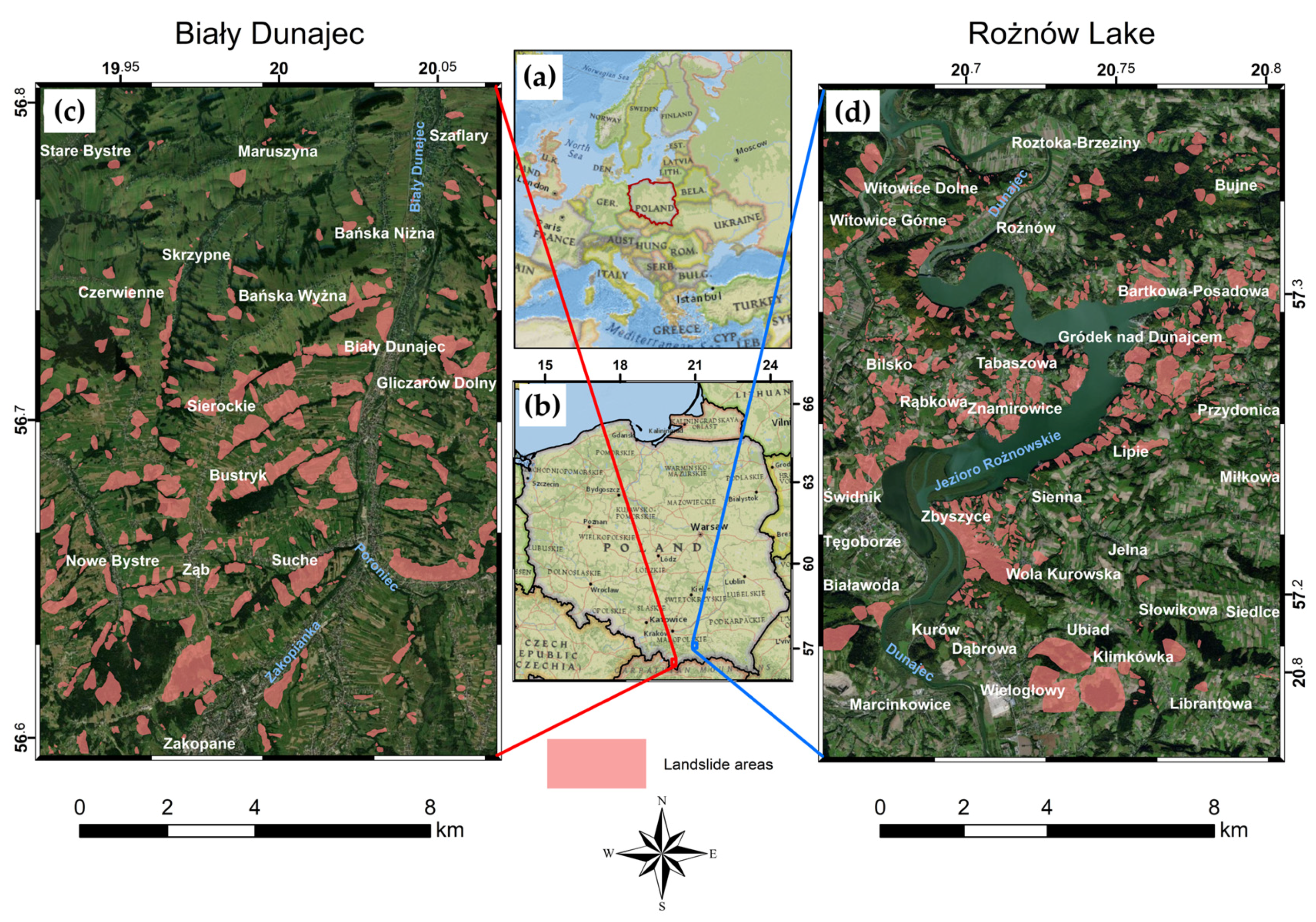
Figure 1. Locations of the study cases (a,b) together with the landslide inventory maps for the first study case, named Biały Dunajec, (c) and the second study case, named Rożów Lake (d).
Applsci 15 08955 g001
Figure 2. Flowchart of methodology adopted in this study.
Applsci 15 08955 g002
Figure 3. Pearson correlation matrix between each LCF and the “target” layer (landslides) for the Biały Dunajec case study.
Applsci 15 08955 g003
Figure 4. Pearson correlation matrix between each LCF and the “target” layer (landslides) for the Rożnów area.
Applsci 15 08955 g004
Figure 5. Normalized feature importance scores for Biały Dunajec (a) and Rożnów (b) case studies.
Applsci 15 08955 g005
Figure 6. Landslide susceptibility maps generated for Biały Dunajec case study (ac) and Rożnów case study (df) for Pearson method (a,d), ANOVA (b,e), and SU (c,f).
Applsci 15 08955 g006
Figure 7. ROCs for Biały Dunajec case study (a) and Rożnów case study (b). Green line for ANOVA in (a) is overlapped by red line.
Applsci 15 08955 g007
Table 1. All input data used for LCF generation and their types and sources.
DataData TypeSourceLink
1.DEMRasterISOKhttps://www.geoportal.gov.pl (accessed on 8 August 2025)
2.Geology mapsRasterPGIhttps://geolog.pgi.gov.pl/ (accessed on 8 August 2025)
3.Soil suitability mapsRasterMIIPhttps://mapymalopolski.pl/app/mapa/miip/1f402b8a-47c0-6894-4ed2-d4ef71d84ede/ (accessed on 8 August 2025)
4.Satellite imagesRasterSentinel-2https://browser.dataspace.copernicus.eu/ (accessed on 8 August 2025)
5.Road networkShapefileOSMhttps://download.geofabrik.de/ (accessed on 8 August 2025)
6.River networkShapefileOSMhttps://download.geofabrik.de/ (accessed on 8 August 2025)
7.PrecipitationPointsIMGWhttps://danepubliczne.imgw.pl/ (accessed on 8 August 2025)
Table 3. LCFs rejected from further investigation based on the analyzed feature selection methods.
Biały Dunajec Case StudyRożnów Case Study
MethodNo. of Rejected FeaturesNo. of Preserved FeaturesRejected FeaturesNo. of Rejected FeaturesNo. of Preserved FeaturesRejected Features
PCC617Curvature, curvature planar, curvature
profile, river proximity, soil texture, TPI
320Curvature, curvature planar, curvature
profile
ANOVA1013Aspect, curvature, curvature planar,
curvature profile, flow direction, LC, main
geological units, river proximity, TPI
617Curvature profile, DEM, curvature,
curvature planar, precipitation, road proximity
SU914CTI, curvature, curvature planar, DEM, fault
proximity, IMI, river proximity, thrust
proximity, TPI
320River proximity, CTI, IMI
Table 4. Accuracy assessment results for Biały Dunajec (BD) and Rożnów (R) case studies.
Feature Selection Method
MeasurePearsonBDANOVABDSUBDPearsonRANOVARSUR
Accuracy0.930.930.900.930.910.93
Precision0.660.650.570.690.620.67
Recall0.930.930.890.940.920.93
F10.770.760.690.790.740.78
AUC0.9850.9810.9810.9830.9720.980
Table 5. Accuracy assessment for the presented study compared to some related works found in the literature.
MethodTraining–Testing RatioFeature ListFeature SelectionOverall AccuracyPrecisionRecallF1-ScoreAUC
Wang et al., 2021 [36]XGBoost70–30%Slope, aspect, altitude, lithology, average annual rainfall, distance to rivers, HI, TWI, NDVI, distance to roads, distance to villages, curvaturePearson correlation coefficient0.7840.8020.7580.7790.860
Sahin, 2020 [33] XGBoost70–30%Slope, elevation, TWI, STI, drainage density, lithology, NDVI, LULC, SPI, aspect, distance to rivers, TRI, TPI, plan curvature, profile curvatureSU0.875---0.957
Pradhan and Kim, 2020 [48] XGBoostTwo areas for training and testingAspect, elevation, slope, curvature, drainage proximity (horizontal), drainage proximity (vertical), SPI, STI, TWI, forest, soil, geologyVariance inflation0.740.600.700.6570.740
Can et al., 2021 [63] XGBoost80–20%Lithology, altitude, TWI, slope orientation, slope gradient, drainage density, plan curvature, SPI, profile curvature-0.900.860.910.880.96
This work, Biały Dunajec case studyXGBoost70–30%DEM, aspect, slope, flow direction, CTI, IMI, SEI, stream proximity, precipitation, tectonics, fault proximity, thrust proximity, road proximity, soil suitability, soil type, NDVI, land coverPCC0.930.650.930.770.985
This work, Roźnów case studyXGBoost70–30%DEM, aspect, slope, flow direction, CTI, IMI, TPI, SEI, stream proximity, precipitation, tectonics, fault proximity, thrust proximity, road proximity, river proximity, soil suitability, soil texture, soil type, NDVI, land coverPCC0.930.690.940.790.980
Disclaimer/Publisher’s Note: The statements, opinions and data contained in all publications are solely those of the individual author(s) and contributor(s) and not of MDPI and/or the editor(s). MDPI and/or the editor(s) disclaim responsibility for any injury to people or property resulting from any ideas, methods, instructions or products referred to in the content.