Abstract
Accurate prediction of coal demand is essential for optimizing energy resources in long-term power system planning. This paper examines the coal demand in North China from 2007 to 2022 using econometric methods to identify key influencing factors as input variables. Then, the Sparrow Search Algorithm (SSA) is used to optimize the key parameters of the Least Squares Support Vector Machine (LSSVM) algorithm to enhance the prediction accuracy of coal demand. Case studies are conducted on actual data in North China, and the results show that the proposed hybrid SSA and LSSVM method outperforms traditional approaches in small-sample, multivariable forecasting, making it suitable for predictions in long-term power system planning.
1. Introduction
Coal resource endowment underpins its strategic role in China’s energy landscape. By 2022, non-fossil energy reached 49.6% of the installed capacity in the power sector, accelerating the substitution of coal power. However, the random volatility of renewable energy increases the uncertainty in the long-term planning of the power systems, raising the difficulty of unit commitment for coal power plants to ensure safety and flexibility. Accurate forecasting of coal demand is essential for developing effective coal strategies in power system planning. This paper develops an intelligent forecasting model to predict long-term coal demand that provides critical support for long-term power system planning.
Existing forecasting methods can be categorized into traditional statistics-based models, single machine-learning models, and combined intelligent models. Traditional forecasting models include time series, elasticity coefficient, and error correction-based approaches. For instance, Rybak, A et al. applied ARIMA and GM models to predict coal demand in various Chinese regions from 2017 to 2025, finding that coal demand targets could be met, but the pressure for its expansion remained [1]. Jiang, S et al. also used ARIMA to predict China’s coal demand, with ARIMA providing the best results [2]. The elasticity coefficient method, developed by Teng, M., et al., forecasted China’s coal demand from 2010 to 2020, while the error correction method [3], adopted by Jia et al., improved the GM model’s accuracy with Hidden Markov Chain corrections [4]. Single machine learning-based models, such as artificial neural networks (ANNs), Support Vector Machines (SVMs), wavelet analysis, and genetic algorithms, have also been used. For example, Liu, Y et al. employed BP neural networks to predict the coal demand and emissions from 2014 to 2020, showing an ongoing rise in consumption and carbon emissions [5]. Li, S et al. combined Grey–Markov chains to predict coal demand in Gansu Province, achieving 92% accuracy but struggling with policy-induced structural breaks [6]. Elasticity coefficient models, as applied by Yan, W et al., faced challenges in addressing multicollinearity among variables like GDP and energy intensity [7]. However, these individual models have limitations in stability and performance across datasets.
Some research efforts combined prediction optimization models by leveraging various intelligent algorithms to optimize traditional models. For example, Yuan et al. used an LSSVM-based model whose parameters are optimized by the gravity search algorithm for short-term prediction of wind power generation, showing superior results compared to single models [8]. Zhang X., et al. utilized BP neural networks to forecast coal consumption, reducing RMSE by 18% compared to ARIMA. However, single-algorithm models often suffer from overfitting in small-sample scenarios, as noted in Tianjin’s case study [9]. Yuan et al. optimized LSSVM parameters using the Gravity Search Algorithm (GSA) for wind power forecasting, inspiring similar applications in coal demand [10]. Similarly, Malvoni et al. used a quadratic Renyi model combined with principal component analysis and LSSVM for wind power load prediction, achieving better performance in various conditions [11]. However, traditional models often require large sample sizes and struggle with abnormal data, while single intelligent algorithms, such as ANNs and SVMs, may face challenges with accuracy and training time.
To overcome these limitations, this paper proposes a novel algorithm for coal demand forecasting by analyzing historical data from five provinces in North China and incorporating social and environmental factors. The proposed econometric method is used to identify the quantitative relationship between influencing factors affecting forecasting accuracy. Additionally, parameter optimization is adopted for the LS-SVM method using the SSA algorithm, which enhances prediction accuracy, particularly for small-sample multivariate forecasting, making it suitable for long-term power system planning. This study aims to develop a hybrid SSA-LSSVM model that integrates econometric causality testing with swarm intelligence to address the challenges of small-sample, multivariable coal demand forecasting in long-term energy planning.
2. Key Factors Affecting Coal Demand
- (1)
- Gross Domestic Product (GDP) per Capita
GDP per capita is defined as the ratio of the total value of final products and services produced by all resident units of a country (or region) over a certain period to the population within the country (or region). As coal is a major energy source, its consumption is influenced by the level of national economic development. Since GDP per capita also affects economic growth, it is important to consider this factor when forecasting coal demand.
- (2)
- CO2 Emissions per Capita
Under the carbon peaking and carbon neutralization policy framework, also known as the “Dual-Carbon” policy in China, CO2 emissions per capita, which are affected by coal demand, have a negative effect on coal demand. This is primarily because China’s carbon emission authorities are actively promoting the formulation and enforcement of the “carbon tax”. This initiative encourages industries and individuals with high carbon emissions to reduce fossil fuel consumption by replacing energy-consuming equipment, improving production processes, and adopting other measures voluntarily. As a result, this helps curb the growth of coal demand by reducing the consumption of fossil energy and CO2 emissions.
- (3)
- Energy Consumption Intensity
Energy consumption intensity is defined as the ratio of energy consumption to GDP, which serves as a good indicator of energy efficiency. From 2007 to 2022, energy consumption intensity in Beijing, Tianjin, and Hebei declined steadily, with only a slight rebound in a few years. This indicates a significant improvement in the quality of economic development in these regions. In contrast, the decline in energy consumption intensity in Inner Mongolia and Shaanxi provinces has been less noticeable, with some minor rebounds in recent years, suggesting a need for further transition toward high-quality development. A decline in energy intensity signals a shift away from fossil energy dependence in economic growth, which suppresses the rise in coal demand.
- (4)
- Industrial Structure
The secondary industry has long been a crucial driver of economic growth in China and remains the dominant source of coal demand. The four major energy-intensive sectors, including electricity, steel, building materials, and chemicals, collectively account for over 90% of China’s coal demand, with the proportion continuing to rise between 2015 and 2022 [12]. Although there has been a gradual decline in the share of the secondary industry in GDP due to ongoing structural adjustments in the national economy, China remains in the midst of industrialization. In this study, the proportion of the secondary industry within the national economy is treated as an independent variable to assess its influence on coal demand.
- (5)
- Urbanization Rate
Urbanization rate is defined as the proportion of the urban population relative to the total population. A notable upward trend across most provinces in North China in recent years has been observed. The exception is Beijing, where strict household registration policies limit migration. This increasing urbanization signifies a substantial migration of rural labor to urban areas, which in turn fosters the expansion of energy-intensive sectors, such as construction and manufacturing. A significant body of literature has established that urbanization in China has been a key driver of coal demand growth [12]. Consequently, the urbanization rate is incorporated as a relevant factor in this analysis.
- (6)
- Energy Structure
China’s resource endowment, characterized by an abundance of coal and the relative scarcity of oil and natural gas, has positioned coal as a dominant energy source within the national energy consumption matrix. In alignment with the goals of promoting ecological civilization, significant progress has been made in cities like Beijing and Tianjin, where policies aimed at reducing coal demand have yielded noticeable results. Similarly, Hebei Province has made strides in adjusting its energy structure. However, regions such as Shaanxi and Inner Mongolia continue to rely heavily on coal, with the proportion of coal in their energy consumption even exhibiting a slight increase in recent years. The ongoing transformation of the energy structure plays a critical role in influencing the coal demand. Thus, the proportion of coal in fossil energy consumption is adopted as a key independent feature for improving the forecasting accuracy [13].
- (7)
- Fossil Energy Consumption
In recent years, the growth rate of fossil energy consumption has slowed due to increasing environmental awareness and rapid development in the new energy sector. The energy production and consumption landscape is gradually shifting from a fossil energy-dominated structure to one increasingly driven by new energy sources [14]. This transition is expected to exert a direct influence on coal demand. Furthermore, coal remains a significant component of fossil energy, and there is likely a notable bidirectional relationship between its consumption and the overall consumption of fossil fuels.
- (8)
- Population Size
Population size is a key determinant of coal demand, as larger population drives higher demand for industrial goods and services, as well as provides a larger labor force for the social production sector. This, in turn, stimulates industrial growth and increases the demand for coal. Additionally, a significant portion of coal demand in China is attributed to residential uses, such as heating and cooking. The consumption of coal for domestic purposes is directly correlated with population size, further reinforcing the relationship between demographic factors and coal demand.
- (9)
- Thermal Power Generation
In the context of the national energy policy of carbon peaking by 2030 and carbon neutralization by 2060, the share of thermal power in China’s energy mix has declined in recent years. However, thermal power generation continues to offer distinct advantages, including low per-kilowatt-hour costs, compact infrastructure requirements, and system stability support. As a result, thermal power will remain a predominant source of electricity in China for the foreseeable future. Coal consumed by thermal power generation accounts for more than half of the total coal demand for commodities, making it a significant and persistent factor influencing coal demand. The model variables are shown in Table 1.

Table 1.
Definition of input and output variables.
3. Least Squares Support Vector Machine (LS-SVM)
As a variant of the Support Vector Machine, LS-SVM simplifies the SVM solution process by using a loss function and converting the quadratic optimization problem into a linear equation system, making the solution process more straightforward. It offers several advantages, including a simpler model, faster solution speed, and no loss of accuracy [15,16].
We let denote the set of training samples, where represents the input variables and represents the outputs. The LS-SVM learning mechanism is formulated through Equation (1), where φ is the input vector and φ(x) represents a mapping function projecting the input features of the original space to a high-dimensional space, ω is the weight vector, and b is the offset value. Thus, such transformation maps the nonlinear regression in input space to a linear problem in the high-dimensional feature space.
The structural risk function is expressed in Equation (2), where defines the model complexity. The parameter C, also referred to as the regularization parameter or penalty factor, quantifies the penalty imposed on errors exceeding the acceptable threshold. Additionally, represents the empirical risk factor.
For minimizing the structural risk, can be formulated as a quadratic expression. Consequently, the regression problem of coal demand forecasting can ultimately be formulated as a constrained optimization problem:
where ξ is the error slack variable, .
By applying the Lagrange multiplier method and dyadic transformation techniques, the above optimization problem can be reformulated into the following Lagrange function, representing an unconstrained optimization problem:
The coefficients of the regression model can be determined by solving the following linear equations derived from the Karush–Kuhn–Tucker (KKT) conditions:
where ; contains l elements. LS-SVM offers Sigmoid, RBF, and polynomial kernel functions to map data into higher dimensions for linear separation. Among these, the RBF kernel function is widely used in practical problems due to its minimal requirement for parameter pre-setting and its adaptability to diverse scenarios. Consequently, the RBF kernel function is adopted in this paper for the LS-SVM model, expressed as
where σ is the kernel width parameter. Finally, the LS-SVM model can be expressed in Equation (8):
where α and b are the parameters that can be determined using the Least Squares method. Furthermore, to enhance the accuracy of the prediction model, two critical parameters must be optimized, including the regularization parameter C and the kernel function parameter σ. In this study, these two parameters are optimized using the Sparrow Search Algorithm (SSA).
4. SSA-Based LS-SVM Model for Coal Demand Forecasting
4.1. LS-SVM Model
When constructing the coal demand prediction model for North China, the selection of characteristic parameters is crucial. An excessive number of parameters can lead to high computational costs, thereby hindering the model’s generalization ability. On the other hand, selecting too few parameters may result in reduced prediction accuracy. Therefore, it is essential to strike a balance in parameter selection to ensure both computational efficiency and predictive accuracy.
Based on the LS-SVM algorithm, the regression model is formulated in Equation (9):
The final prediction output represents the forecasted coal demand across different provinces, with each intermediate node corresponding to a support vector, where x1, x2,…,xn denote the input variables.
4.2. SSA-Optimized LSSVM Prediction Model
In fact, the performance of the LSSVM model for coal demand prediction using RBF as its kernel function is primarily influenced by two critical parameters: the regularization parameter C and the kernel function parameter σ. The regularization parameter C governs the trade-off between the model’s confidence range and the empirical risk. A large value of C imposes a higher penalty for errors during the training of the LSSVM, which can lead to model overfitting, while a smaller value of C reduces the model’s complexity, potentially underfitting the data. On the other hand, σ determines the distribution’s complexity of the sample data in the high-dimensional feature space. A larger value of σ reduces model complexity but increases the risk of overfitting, whereas a smaller value results in a smoother model fit.
In [17], Abualigah, L et al. introduced the Salp Swarm Algorithm (SSA), a novel heuristic optimization approach inspired by the swarming behavior of salps. The SSA divides the population into two groups: (1) Leaders at the front of the chain and (2) Followers trailing behind the leaders. The leader guides the salp chain in the search space, while the followers mimic the leader’s movements, enabling a global search. This chain-based behavior enhances the algorithm’s global optimization capability and reduces the likelihood of converging to local optima.
Inspired by the above work, this paper employs the SSA algorithm to optimize C and σ to enhance the model’s predictive accuracy. The proposed hybrid SSA-LSSVM models for coal demand forecasting are constructed for five provinces in North China. The main steps of the SSA-LSSVM forecasting model are outlined as follows:
- Parameter Settings: The key parameters of the SSA algorithm consist of the number of variables (dim), the maximum number of iterations (Mite), the number of search agents (SAN), the upper bound (ub), and lower bound (lb) of the variables. In this paper, the values are set as follows: SAN = 50, Mite = 300, dim = 2, ub = [100,000; 100,000], and lb = [1; 1].
- Population Initialization: With the above initial parameter settings, a random salp population is created to initiate the iteration process, as described in Equation (10). The initial iteration value is set to 1.
- The Fitness Function: In this study, the SSA-LSSVM model is applied to forecast the coal demand across five provinces in North China. The fitness function is defined by calculating the error between the actual values and the predicted values using the Mean Absolute Percentage Error (MAPE) criterion, as shown in Equation (11).where is the actual coal demand and denotes the forecasted coal demand.
- Optimization Process: Starting with the initial population values, the fitness of all salps is computed, and the position of the salp exhibiting the best fitness is designated as variable F, which must be updated at each iteration. Upon identifying F, both the leader and the follower salps update their positions to converge toward the global optimum.
- Completion of Optimization: The optimal salp position and its corresponding fitness value are obtained at each iteration. When the maximum number of iterations is reached, the optimization process concludes. Subsequently, all fitness values are sorted, and the optimal value is selected. The salp position corresponding to this optimal value is then used to determine the optimal regularization parameter C for the LSSVM model and the optimal kernel function parameter σ for the RBF kernel function, as identified by the SSA method.
The main flowchart of the proposed SSA-LSSVM method for coal demand forecasting in five provinces of North China is illustrated in Figure 1.
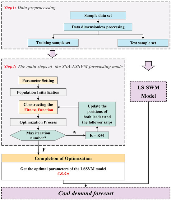
Figure 1.
Framework diagram of coal demand forecasting technology.
5. Case Study
5.1. Data Description
The data utilized in this study, including GDP per capita, CO2 emissions per capita, energy intensity, industrial structure, urbanization rate, energy structure, fossil energy consumption, total population, thermal power generation, and coal demand in the provinces of North China from 2014 to 2024, are obtained from the China Energy Statistical Yearbook (2014–2024) and the reports on the macroeconomic and social development of each region in previous years.
5.2. Granger Causal and Correlation Tests
Stock, J.H et al. showed that causality tests are highly sensitive to time series stability [18]. The initial step is to perform a stationarity test on the time series data of the influencing variables and coal demand. The Augmented Dickey–Fuller (ADF) values for the selected factors significantly exceed the critical value of 0.05, indicating that these five variables are second-order stationary series. Due to space constraints, the detailed ADF test procedure is omitted in this paper. From Table 2, the Granger causality test results reveal the following relationships:
- A.
- GDP per capita (x1) is found to be Granger causal for coal demand in North China with a second-order lag at a 0.1 confidence level. However, coal demand (y) exhibits Granger causality for GDP per capita in certain provinces.
- B.
- Carbon dioxide emissions per capita (x2) is a Granger cause for coal demand, while coal demand (y) is also found to Granger cause carbon dioxide emissions in some provinces.
- C.
- Urbanization rate (x4) in North China is Granger causal for coal demand in some provinces, but coal demand (y) is not a Granger cause of the urbanization rate.
- D.
- Industrial structure (x5) is Granger causal for coal demand in North China, suggesting that industrial restructuring influences coal demand. However, the reverse causality, where coal demand drives changes in industrial structure, does not hold.
- E.
- Total population (x8) exhibits Granger causality for coal demand, but coal demand (y) is not Granger causal for population changes. This suggests that, given China’s large population base, population growth is more responsive to coal demand than vice versa.
- F.
- Thermal power generation (x10) and coal demand have bidirectional Granger causality, indicating a mutual relationship where thermal power generation and coal demand influence each other.
Table 2.
Results of the Granger Causality Test.
Table 2.
Results of the Granger Causality Test.
| Lagged Order | Beijing | Hebei | Neimenggu | Shanxi | Tianjin | |
|---|---|---|---|---|---|---|
| y is not x1 Granger dependent variable | 2 | 0.99 | 0.0794 | 0.0022 | 0.5352 | 0.3045 |
| x1 is y Granger dependent variable | 2 | 0.0715 | 0.0766 | 0.0602 | 0.0313 | 0.0111 |
| y is not x2 Granger dependent variable | 2 | 0.3132 | 0.062 | 0.0486 | 0.0884 | 0.1471 |
| x2 is y Granger causal variable | 2 | 0.0159 | 0.3999 | 0.0544 | 0.0032 | 0.0469 |
| y is x4 Granger causal variable | 2 | 0.0736 | 0.0224 | 0.0227 | 0.0833 | 0.155 |
| x4 is not y Granger causal variable | 2 | 0.4825 | 0.1009 | 0.0211 | 0.4041 | 0.736 |
| y is not x5 Granger causal variable | 2 | 0.8769 | 0.7981 | 0.3801 | 0.6969 | 0.928 |
| x5 is y Granger causal variable | 2 | 0.085 | 0.0708 | 0.0547 | 0.0742 | 0.0178 |
| y is not x8 Granger causal variable | 2 | 0.1495 | 0.6529 | 0.0549 | 0.8432 | 0.4965 |
| x8 is y Granger causal variable | 2 | 0.2174 | 0.0394 | 0.0449 | 0.627 | 0.5802 |
| y is not x9 Granger causal variable | 2 | 0.0758 | 0.0338 | 0.0139 | 0.0609 | 0.0441 |
| x9 is y Granger causal variable | 2 | 0.0885 | 0.0455 | 0.0329 | 0.0145 | 0.0556 |
These results highlight the complex interplay between economic, demographic, and industrial factors in shaping coal demand patterns in North China.
In addition, a correlation analysis is conducted with results shown in Table 3. It can be observed that the three variables x3 (energy intensity), x6 (energy structure), and x7 (fossil energy consumption) exhibit no significant correlation with y (coal demand). As a result, these variables are excluded from the subsequent multicollinearity test.
Table 3.
Variable correlation.
5.3. Performance of the Proposed Model and Discussion
- (1)
- SSA Parameter Optimization
The optimization of the LS-SVM model using the SSA optimization algorithm involves prior training and prediction of the sample set. Through this process, the combinations of model parameters C and σ are automatically optimized, leading to the identification of the optimal parameter combinations under low fitness conditions. In this study, the SSA optimization algorithm is employed, and the RBF kernel function is used for parameter optimization. After 300 iterations, the parameter optimization process is automatically terminated. At iteration 293, the fitness value reaches , indicating a high model fitting accuracy. The convergence curve further demonstrates that the SSA algorithm exhibits high convergence efficiency and fast operation speed. Thus, the resulting LS-SVM parameter combinations are considered optimal at this stage.
- (2)
- Evaluation Metrics
This study employs three error evaluation metrics—Mean Absolute Error (MAE), Root Mean Square Error (RMSE), —to assess the prediction accuracy of the SSA-LSSVM model. These metrics are calculated as follows:
where
represents the length of the test set, denotes the dimensionless actual values, and corresponds to the dimensionless predicted values. MAE and RMSE serve as indicators of the magnitude of the actual error and the residual sum of squares, respectively, with both metrics in the range of [0, +∞). A value closer to 0 indicates higher model accuracy. The value of lies within the range of (−∞, 1], with values closer to 1 indicating a better fit between the predicted and actual values.
To further validate the superiority of the SSA-LSSVM model, comparisons are made with three other models: Support Vector Regression (SVR), Random Forest (RF), and the Boosting Algorithm. Similar to the SSA-LSSVM model, the three comparison models are trained using a fixed 4:1 ratio for partitioning the dataset into training and testing sets. The normalized predicted results and actual values are then substituted into Equations (12)–(14) to compute the MAE, RMSE, and for each model. The error analysis metrics for the training set with the highest prediction accuracy for each model are then compared with those of the SSA-LSSVM model to assess its relative effectiveness.
- (3)
- Prediction Results and Analysis
The error evaluation indices obtained by the SSA-LSSVM model are presented in Table 4, Table 5, Table 6, Table 7 and Table 8. These results indicate that the prediction outcomes from the SSA-LSSVM model align closely with the actual data, demonstrating a high level of accuracy. Specifically, the model exhibits low error rates, confirming its effectiveness in capturing the underlying trends in coal demand across the provinces. The consistent performance across different regions further supports the model’s robustness and potential for broader application in coal demand forecasting.
Table 4.
Comparison of the errors of various models of Beijing coal demand.
Table 5.
Comparison of the errors of various models of Hebei coal demand.
Table 6.
Comparison of the errors of various models of Neimenggu coal demand.
Table 7.
Comparison of the errors of various models of Shanxi coal demand.
Table 8.
Comparison of the errors of various models of Tianjin coal demand.
The error evaluation indices of the SSA-LSSVM model, along with the optimal results of each comparison model obtained through 20 iterations of random partitioning, are presented in Table 4, Table 5, Table 6, Table 7 and Table 8. These results demonstrate that the SSA-LSSVM model exhibits smaller errors and superior prediction performance compared to the SVR, RF, and Boosting models. In the research and application of long-term series prediction, the challenge of generalization performance is particularly significant. The adaptability of the model to new samples, new features, or new data distributions is limited. Although the accuracy of the model proposed in this article may not be optimal for every set of data, overall, it is accurate. This suggests that the SSA-LSSVM model provides more accurate coal demand predictions and holds higher practical value.
5.4. Coal Demand Forecasting Result
Based on data from the China Statistical Yearbook and analysis results of the Granger causality test, this study compares the elastic relationships among GDP, coal prices, industrial structure, and coal demand from 2014 to 2024. Within a defined range of variation, elasticity-based predictions for coal demand are implemented.
- (1)
- Gross National Product (GNP) ForecastThe elasticity-based GNP forecast estimates potential fluctuation ranges for future GNP based on GDP growth rates. Given China’s economic “new normal” characteristics and referencing the 13th Five-Year Plan for National Economic and Social Development [19], which set a goal of “doubling the 2010 GDP by 2020”, along with analyses and projections from research institutions on national accounting indicators, the GDP growth rate for 2025–2030 is projected at 6.8–7%, with an elasticity variation reference of 0.1%.
- (2)
- Coal Consumption Share ForecastBased on data availability, China’s proportion of coal consumption in primary energy use showed a declining trend from 2019 to 2024, with an annual average growth rate ranging from −0.2% (maximum) to −3.4% (minimum). This study defines the annual growth rate fluctuation range for coal consumption share during 2025–2030 as [−3.2, −0.4%].
- (3)
- Coal Utilization Efficiency ForecastAssuming data from the study period (2019–2024), the annual growth rate of industrial value-added contributed by unit coal consumption in China reached 5.1–6.9%. This range is adopted as the projected annual growth rate interval for industrial value added generated by coal consumption during 2025–2030.
- (4)
- Clean Energy Consumption Share ForecastHistorical data indicate that the annual growth rates of natural gas, wind power, hydropower, and nuclear power ratios in China increased steadily from 2019 to 2024, with a maximum annual growth rate of 5.6% and a minimum of 0.6%. For 2025–2030, the energy substitution effect is projected to rise by 0.6–5.6 percentage points.
- (5)
- Industrial Value-Added-to-GDP Ratio ForecastReferencing the 2017 Analysis and Forecast of China’s Macroeconomic Situation [20], the ratio of secondary industry output to GDP is projected to reach 40.5–46.4% during 2025–2030. Given that the ratio of industrial value added to secondary industry output remained 88.05% throughout the study period, China’s industrial value-added-to-GDP ratio for 2019–2024 is estimated at 35.66–40.86%.
- (6)
- Coal Price ForecastNon-coal factors (e.g., transportation bottlenecks) significantly impact coal prices. Additionally, under China’s proactive coal industry strategy amid resource and environmental protection efforts, policies such as environmental damage costs, coal safety costs, and resource tax reforms inevitably affect cost-driven coal price increases. Based on historical data (2019–2024), the annual growth rate of coal ex-factory prices varied by 0.31–0.52 percentage points.
To project coal demand for 2025–2030, GDP growth rates are categorized into low, medium, and high scenarios. The other six factors are assigned random minimum or maximum growth values. For each GDP scenario, 64 (26) possible fitted values are generated annually, from which the minimum and maximum values are selected as the upper and lower bounds for coal demand. The results of China’s total coal demand projections for 2025–2030 are summarized in Figure 2.
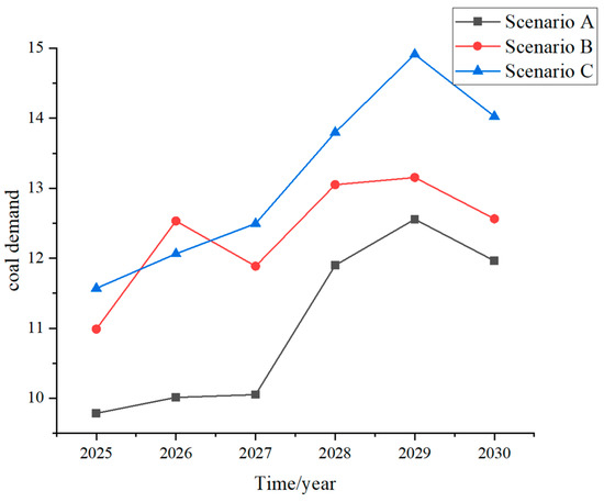
Figure 2.
Coal demand forecasting result.
It can be seen from the above figure that Scenario A and Scenario B have always shown a relatively rapid downward trend since 2018, while Scenario C is slowly rising first and then slowly decreasing, and the overall situation is relatively flat. Scenario C best fits the trend of China’s energy planning development. When the economy is at a relatively low speed, the carbon emissions per unit of GDP are at a higher rate decline, and the scientific and technological progress is at a relatively slow level, China’s coal consumption is relatively slow declining. Based on the actual situation, China’s coal consumption is in a slow growth trend, which is more consistent with the forecast of Scenario C. This shows that China’s current economic development is in the process of transitioning from high-speed development to high-quality one, and the speed has slowed down; China’s unit GDP carbon emissions are on a rapid decline, and China’s carbon emission reduction efforts have been continuously strengthened. China’s scientific and technological progress has maintained a steady growth rate. This development status is also relatively consistent with the development trend planned by the Chinese government. China’s energy development “13th Five-Year Plan” pointed out that in 2020, the total energy consumption was controlled within 5 billion tons of standard coal, and the total coal consumption was controlled within 4.1 billion tons. The total coal consumption increased by 0.7% annually. The China Energy Outlook 2030 report is expected to be around 3.6 billion tons in 2030. Based on 2015, the average annual growth rate of coal consumption is −0.52%.
6. Conclusions
To effectively support power system planning and enable more flexible and reliable unit commitment (UC) arrangements for coal power plants, this paper proposes a robust forecasting method for predicting future coal demand in the power system. By identifying and verifying the key factors influencing coal demand, this study broadens the scope of factor selection from economic, social, and environmental perspectives. The paper introduces carbon emissions per unit of GDP, industrial structure, and thermal power generation as new indicators, in addition to traditional economic and demographic factors.
Furthermore, the paper innovatively applies econometric principles to analyze the causal relationships among these variables. This approach enhances the accuracy of the prediction model by better understanding the correlations between explanatory variables and the causal relationships of the dependent variables.
Additionally, the traditional Support Vector Machine (SVM) is enhanced, and an SVM model optimized through the Salp Swarm Algorithm (SSA) is proposed. This optimization reduces the model’s dependency on sample size, making it particularly well suited for long-term power system forecasting needs. Based on the results of this study, the following conclusions can be drawn:
- The SSA-optimized LSSVM algorithm proposed in this paper outperforms traditional forecasting methods in terms of prediction accuracy. It demonstrates superior performance compared to single intelligent learning methods while also being suitable for small-sample predictions, given the limited number of samples.
- At the application level, the SSA-LSSVM algorithm outperforms Support Vector Regression (SVR), Random Forest (RF), and Boosting models in short-term predictions. In terms of prediction effectiveness, the proposed algorithm also exhibits a clear advantage in long-term forecasting.
Author Contributions
W.S.: Conceptualization, Writing–original draft. Z.S.: Project administration, Writing–review & editing. A.W.: Methodolog. R.D. Writing–review & editing. G.X.: Project administration. S.S. Writing–review & editing. All authors have read and agreed to the published version of the manuscript.
Funding
This research was funded by the 75th batch of general funding from the China Postdoctoral Science Foundation grant number [2024M75284].
Institutional Review Board Statement
Not applicable.
Informed Consent Statement
Not applicable.
Data Availability Statement
The raw data supporting the conclusions of this article will be made available by the authors on request.
Conflicts of Interest
Authors Wentao Sun and Shan Song were employed by the company State Grid Jiangsu Electric Power Co., Ltd., Economic Research Institute. The remaining authors declare that the research was conducted in the absence of any commercial or financial relationships that could be construed as a potential conflict of interest.
References
- Rybak, A.; Manowska, A.A. The forecast of coal sales taking the factors influencing the demand for hard coal into account. Gospod. Surowcami Miner. 2019, 35, 129–140. [Google Scholar] [CrossRef]
- Jiang, S.; Yang, C.; Guo, J.; Ding, Z. ARIMA forecasting of China’s coal consumption, price and investment by 2030. Energy Sources Part B Econ. Plan. Policy 2018, 13, 190–195. [Google Scholar] [CrossRef]
- Teng, M.; Burke, P.J.; Liao, H. The demand for coal among China’s rural households: Estimates of price and income elasticities. Energy Econ. 2019, 80, 928–936. [Google Scholar] [CrossRef]
- Jia, Z.; Zhou, Z.; Zhang, H.; Li, B.; Zhang, Y.X. Forecast of coal consumption in Gansu Province based on Grey-Markov chain model. Energy 2020, 199, 117444. [Google Scholar] [CrossRef]
- Liu, Y.; Du, R.; Niu, D. Forecast of coal demand in shanxi province based on GA—LSSVM under Multiple Scenarios. Energies 2022, 15, 6475. [Google Scholar] [CrossRef]
- Li, S.; Li, R. Comparison of forecasting energy consumption in Shandong, China Using the ARIMA model, GM model, and ARIMA-GM model. Sustainability 2017, 9, 1181. [Google Scholar] [CrossRef]
- Yan, W.; Jingwen, L. China’s present situation of coal consumption and future coal demand forecast. China Popul. Resour. Environ. 2008, 18, 152–155. [Google Scholar] [CrossRef]
- Yuan, X.; Chen, C.; Yuan, Y.; Huang, Y.; Tan, Q. Short-term wind power prediction based on LSSVM–GSA model. Energy Convers. Manag. 2015, 101, 393–401. [Google Scholar] [CrossRef]
- Zhang, X.; Liu, C.; Qian, Y. Coal price forecast based on ARIMA model. Financ. Forum 2020, 9, 180. [Google Scholar] [CrossRef]
- Yuan, X.; Tan, Q.; Lei, X.; Yuan, Y.; Wu, X. Wind power prediction using hybrid autoregressive fractionally integrated moving average and least square support vector machine. Energy 2017, 129, 122–137. [Google Scholar] [CrossRef]
- Malvoni, M.; Giorgi, M.D.; Congedo, P.M. Photovoltaic forecast based on hybrid PCA–LSSVM using dimensionality reducted data. Neurocomputing 2016, 211, 72–83. [Google Scholar] [CrossRef]
- Duan, H.; Luo, X. A novel multivariable grey prediction model and its application in forecasting coal consumption. ISA Trans. 2022, 120, 110–127. [Google Scholar] [CrossRef] [PubMed]
- Ji, Q.; Zhang, D. How much does financial development contribute to renewable energy growth and upgrading of energy structure in China? Energy Policy 2019, 128, 114–124. [Google Scholar] [CrossRef]
- Jiang, P.; Yang, H.; Ma, X. Coal production and consumption analysis, and forecasting of related carbon emission: Evidence from China. Carbon Manag. 2019, 10, 189–208. [Google Scholar] [CrossRef]
- Suykens, J.A.K.; Vandewalle, J. Least Squares Support Vector Machine Classifiers. Neural Process. Lett. 1999, 9, 293–300. [Google Scholar] [CrossRef]
- Baesens, B.; Viaene, S.; Van Gestel, T.; Suykens, J.; Dedene, G.; De Moor, B.; Vanthienen, J. Least Squares Support Vector Machine Classifiers: An Empirical Evaluation; Katholieke Universiteit Leuve: Leuven, Belgium, 2000; pp. 1–16. [Google Scholar]
- Abualigah, L.; Shehab, M.; Alshinwan, M.; Alabool, H. Salp swarm algorithm: A comprehensive survey. Neural Comput. Appl. 2020, 32, 11195–11215. [Google Scholar] [CrossRef]
- Stock, J.H.; Watson, M.W. Evidence on structural instability in macroeconomic time series relations. J. Bus. Econ. Stat. 1996, 14, 11–30. [Google Scholar] [CrossRef]
- The Central Compilation Group of the Communist Party of China Outline of the 13th Five Year Plan for National Economic and Social Development of the People’s Republic of China; People’s Publishing House: Beijing, China, 2016.
- Li, Y. Analysis and Forecast of China’s Economic Situation in 2017; Social Sciences Literature Press: Beijing, China, 2016. [Google Scholar]
Disclaimer/Publisher’s Note: The statements, opinions and data contained in all publications are solely those of the individual author(s) and contributor(s) and not of MDPI and/or the editor(s). MDPI and/or the editor(s) disclaim responsibility for any injury to people or property resulting from any ideas, methods, instructions or products referred to in the content. |
© 2025 by the authors. Licensee MDPI, Basel, Switzerland. This article is an open access article distributed under the terms and conditions of the Creative Commons Attribution (CC BY) license (https://creativecommons.org/licenses/by/4.0/).