Abstract
Vehicle suspension significantly influences the safety of cargo transportation. This study presents a 14-degree-of-freedom vehicle–cargo coupling model that explicitly incorporates the frequency-dependent stiffness of air springs. Systematic parametric investigations of air spring orifice resistance, loading mass, and cargo stiffness reveal the following: (a) Compared with leaf spring suspension, air suspension vehicles attenuated the first peak of acceleration power spectral density by over 50%, while slightly amplifying the second peak; (b) When replacing leaf spring suspension with air suspension, the upper-layer cargo exhibited significantly larger vibration reductions (14% vertical, 28% pitch) than the lower-layer cargo under identical cargo parameters. The roll angle should be controlled to prevent the cargo overturning when equipping air suspensions; (c) Under light loading conditions, the vertical vibration response in upper-layer cargo is amplified. This amplification can be effectively suppressed through two complementary approaches, i.e., employing low-stiffness cushion materials and reducing orifice resistance through tunable orifices, which collectively attenuate characteristic peaks in the frequency-domain response and comprehensively mitigate the vertical vibration of cargo. These findings provide guidance for designing transportation schemes for cargo in air suspension vehicles to enhance cargo safety.
1. Introduction
Within modern logistics systems, the efficiency and safety of vehicle transportation are critical, and these significantly influence economic development. Key vehicle subsystems such as the chassis [1], suspension [2], and tires [3] exert a profound influence on these performance metrics. Among these subsystems, the suspension system functions as the primary vibration isolation component, playing a vital role in ride comfort and stability. This system is particularly critical for logistics operations, as it directly governs the dynamic loads imposed on cargo and overall transportation safety. Therefore, examining suspension characteristics and their impact on the dynamic response of cargo is valuable in research and practice. This work helps optimize transport packaging system design and balance protective effectiveness against economic costs.
Air spring suspensions significantly improve vehicle ride comfort due to their unique advantages, including adjustable stiffness, low natural frequency, and excellent vibration isolation performance [4,5]. Consequently, their application is increasingly expanding into freight transport vehicles. Air suspension modeling targets vertical dynamics to capture its vibration isolation. As the core vibration isolation component, air springs have garnered significant research attention [6,7,8,9,10,11,12,13], particularly regarding their dynamic characteristics. Currently, most air spring models are thermodynamic models derived from the ideal gas equation of state, the gas variable process equation, and fluid mechanics equations. The advantage of such models is the ability to directly guide the design of air spring system parameters. For instance, Quaglia et al. [12] derived a thermodynamic model for air springs based on thermodynamics and fluid mechanics, which further confirmed the distinct frequency-dependent stiffness characteristics. Nieto et al. [13] established nonlinear and linearized models of air spring, validating both models against experimental data. Their findings demonstrate that both models accurately capture the dynamic characteristics of air springs. Therefore, the thermodynamic model serves as an effective tool for characterizing air spring and thus predicts overall suspension performance.
In order to investigate the dynamic characteristics of vehicles incorporating air suspension models, two primary modeling approaches prevail: multi-body dynamics simulation [14,15] and lumped-parameter multi-degree-of-freedom (MDOF) modeling [16,17,18,19,20,21]. The MDOF modeling approach derives governing equations of motion via Newton’s law or Lagrange’s equations, providing an efficient and physically interpretable framework for dynamic analyses of air suspension vehicles. This approach exhibits flexibility in embedding the dynamic characteristics of air springs within dynamic analyses of vehicles. Consequently, this study adopts the MDOF modeling approach due to these advantages.
However, existing MDOF studies on air suspension vehicles exhibit significant limitations. These studies focus almost exclusively on vehicle performance metrics while disregarding cargo. For instance, Moheyeldein et al. [18] employed a quarter-vehicle model to compare the vibration reduction performance of air suspensions versus passive suspensions, demonstrating superior ride comfort in air suspension vehicles. However, this simplified model inherently neglected cargo. Separately, Le et al. [19] established a 14-degree-of-freedom model including cargo. While this model boasts considerable complexity in representing the vehicle, it treats the cargo as lumped rigidly with the vehicle body, thereby ignoring the essential dynamic coupling effects between the cargo and the vehicle. Consequently, there remains limited understanding of how unique dynamic properties of air suspension vehicles influence cargo dynamic response and potential damage risks during transport operations.
In cargo transport packaging design, the core challenge lies in accurately predicting dynamic cargo responses under transport conditions to balance protective requirements against over-packaging. Research efforts have consequently focused on analyzing cargo vibration characteristics [22,23,24,25,26,27]. These studies recognize the significant influence of vehicle–cargo coupling effects and spatial distribution factors on dynamic response. For example, Huang et al. [26] developed a vehicle–cargo coupling model elucidating vibration transmission mechanisms, though it was limited to vehicles with traditional leaf spring suspensions. Molnár et al. [27] analyzed vibration acceleration in triple-stacked packaging units during transport simulations and field testing, demonstrating escalating vibration intensity with increased stacking height. However, these studies into the vibration responses of cargo neglect the increasing adoption of air suspension systems and their unique dynamic behaviors.
Collectively, current research exhibits limitations in two key areas. Firstly, research on air suspension vehicle dynamics concentrates primarily on vehicle performance metrics themselves while neglecting cargo response influences, and it often employs oversimplified models that inadequately capture realistic coupling effects. Secondly, research on cargo vibration, though incorporating vehicle–cargo coupling and spatial distribution factors, rarely accounts for the impacts of air spring suspension.
To bridge these gaps, this study addresses the following central questions: How does the frequency-dependent stiffness of air springs influence vehicle–cargo dynamics, and what parametric strategies mitigate vibration-induced cargo risks? Guided by these objectives, this study proposes three mechanistic hypotheses:
- The frequency-dependent stiffness of air springs significantly influences peaks in the acceleration power spectral density of cargo;
- Compared with leaf spring suspensions, air suspensions provide different vibration reduction effects for upper and lower cargo layers;
- Tuning orifice resistance and cargo parameters suppresses cargo vibration.
To test these hypotheses, this study incorporates the frequency-dependent stiffness characteristics of air spring suspensions to establish a 14-degree-of-freedom (14-DOF) vehicle–cargo coupling model, which contains two layers of cargo. This study also analyzes the influence of the air spring parameter (orifice resistance) and cargo parameters (loading mass and cargo stiffness) on the dynamic response of the model. The findings from this comprehensive modeling and parametric analysis can guide the design of air suspension vehicle transport schemes to improve cargo safety.
2. Vehicle–Cargo Coupling Model
2.1. Model Assumptions
The vehicle–cargo coupling model incorporates the following key assumptions:
- Vehicle motion is restricted to straight-line travel, neglecting yaw dynamics and lateral vibrations;
- The contact forces between cargo and vehicle floor and the interaction forces between cargo layers are represented as uniformly distributed loads. This simplification is valid for stacked palletized cargo under real-world transport conditions;
- All mass components in the model are idealized as rigid bodies. This assumption holds because structural deformations are negligible compared with gross motion displacements;
- Suspension deflection is constrained to small displacements near static equilibrium. This assumption holds because deflection amplitudes typically remain within small working ranges in highway driving simulations.
2.2. Model Establishment
Following the modeling assumptions, a 14-DOF vehicle–cargo coupling model is established (Figure 1). All 14 degrees of freedom defined above are explicitly annotated using red symbols in Figure 1. This model explicitly defines the degrees of freedom allocated to distinct subsystems, as follows:
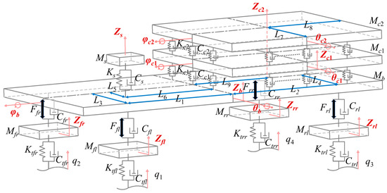
Figure 1.
Structural schematic diagram of a 14-DOF vehicle–cargo coupling model.
- Wheels (unsprung mass): Zfl, Zfr (front left/right vertical displacements); Zrl, Zrr (rear left/right vertical displacements);
- Driver’s seat: Zs (vertical displacement);
- Vehicle body (floor): Zb (vertical displacement), θb (pitch angle), φb (roll angle);
- Lower-layer cargo: Zc1 (vertical displacement), θc1 (pitch angle), φc1 (roll angle);
- Upper-layer cargo: Zc2 (vertical displacement), θc2 (pitch angle), φc2 (roll angle).
All vertical displacements are in meters (m) and all rotational angles are in radians (rad). Road elevation inputs q1 to q4 correspond to excitation profiles at the front-left, front-right, rear-left, and rear-right wheels, respectively. Remaining parameters are defined in Table 1 and Table 2. Notice that unlike conventional lumped stiffness (N·m−1), the cargo distributed stiffness has units of N·m−3, representing equivalent stiffness per unit contact area [26]. The equivalent stiffness is the compression displacement of the cargo cushion under static loading. Similarly, distributed damping is expressed in units of N·s·m−3.

Table 1.
Vehicle parameter values.
Table 2.
Cargo parameter values.
By decoupling the suspension-specific stiffness forces from the overall system stiffness forces, the system governing equation of motion at equilibrium is derived through the damped Lagrange’s equations, as follows:
where the generalized coordinate vector Z(t), stiffness matrix K, damping matrix C, coefficient matrix B1, and external force matrix Q(t) are as defined in the Appendix A, the mass matrix M is a diagonal matrix given by diag(Mfl, Mfr, Mrl, Mrr, Ms, Mb, Ibx, Iby, Mc1, Ic1x, Ic1y, Mc2, Ic2x, Ic2y), and the suspension force vector FS is defined as follows:
where Ffl, Ffr, Frl, and Frr denote the suspension force components of FS, determined by their respective suspension characteristics.
The suspension characteristic models used in this study are as follows:
- For the leaf spring suspension system adopted in this study, the suspension output forces follow a linear force-displacement relationship and are calculated about the static equilibrium using Equation (3), as follows:where Fleaf denotes the leaf spring suspension output force (N), Kij represents the leaf spring’s linear stiffness (N·m−1) with subscripts i (front/rear position) and j (left/right position), and h is the suspension deflection (m);
- Following the modeling approach described in the literature [12,13] for the air spring suspension, this study linearizes the nonlinear model (derived from thermodynamic and fluid dynamic principles) using Taylor series expansion about the static equilibrium position. The linearization process yields the governing equations presented in Equation (4), as follows:where P1 and P2 are the pressures in the main and the auxiliary chamber, respectively (Pa), G is the inter-chamber gas mass flow rate (kg s−1), and Fair denotes the air spring output force (N). The air suspension in this study features two air springs per side, resulting in an output force twice that of a single air spring. Remaining parameters are provided in Table 3.
Table 3. Vehicle rear suspension parameter values.
Notice that the orifice model adheres to the ISO 6358 standard [28] for quasi-static conditions. According to the Reference [12], the orifice resistance RF (the core parameter of the orifice model) is treated as a constant value inversely related to orifice conductance C. As stipulated by ISO 6358, C is positively correlated with the orifice diameter Do (the key parameter for tuning gas flow dynamics). The RF quantifies flow resistance during gas exchange between main and auxiliary chambers. Higher RF values indicate greater flow resistance, consequently restricting gas transfer.
The frequency-dependent characteristics of the linearized model are derived in Section 3.2. Figure 2 shows the air spring model under static equilibrium.
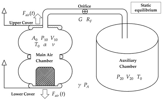
Figure 2.
The air spring model under static equilibrium.
This study utilizes a model based on a Dongfeng truck. In this model, the front suspension retains its original leaf spring configuration, while the rear suspension is modified by replacing the original leaf spring with a commercial air spring [12]. The original leaf spring rear suspension serves as the benchmark for comparison. The parameters of the air spring suspension are specifically matched to the benchmark based on the principle of static equilibrium load. All parameters are detailed in Table 1, Table 2 and Table 3. The parameter values of the model original vehicles and cargo used in this study are taken from Reference [26], while the air suspension parameters are sourced from Reference [12].
The matching rule states that under loaded conditions, the single-side support reaction force FAS of the rear suspension is calculated by , then the operating pressure P10 of the air spring can thus be determined.
2.3. Solution Approaches
The solution accuracy of the model was verified through two independent approaches: Laplace transform approach and Simulink simulation approach. Both of these were used for modeling and computation with MATLAB (R2022a).
2.3.1. Laplace Transform Approach
The Laplace transform applied to differential Equations (1), (3) and (4) gives the following:
where Kair(s) denotes the frequency-dependent stiffness of the air spring, with s being the complex frequency variable from the Laplace transform; KV12 and KV1 represent the stiffness components related to the chamber volume; KA is the stiffness associated with the effective area; and CR signifies the pneumatic capacities of the auxiliary chamber. KV12, KV1, KA and CR are intermediate variables characterizing the dynamic stiffness of air springs in mathematical models, enabling accurate representation of Kair(s).
Consequently, FS(s) in Equation (5) can be expressed as Equation (8):
where the transfer function matrix H(s) is given by diag(Hfl(s), Hfr(s), Hrl(s), Hrr(s)), and the coefficient matrix B2 is defined in the Appendix A. The expression for Hij(s) depends on the suspension type, as follows:
- For leaf spring suspensions: Hij(s) = Kij;
- For air spring suspensions: Hij(s) = 2Kair(s).
Substituting Equation (8) into Equation (5) and rearranging terms yields the following:
The frequency-domain response Z(s) is then obtained from Equation (9). The corresponding time-domain response Z(t) follows via inverse Laplace transform.
2.3.2. Simulink Simulation Approach
The Simulink simulation approach constructs a computational framework in MATLAB/Simulink. By interconnecting functional modules, it establishes the system’s state-space representation to solve for the time-domain response.
The system state vector is defined as follows:
The output vector is defined as follows:
Equation (10) converts the equations of motion (1) into the following state-space form:
where the input vector V is defined by V = Q + B1FS, and the remaining state-space matrices are defined as follows:
The suspension force vector FS is calculated from suspension deflection, which is derived from output vector . Figure 3 shows the methodological framework implementation of the Simulink simulation approach for the 14-DOF vehicle–cargo coupling model.
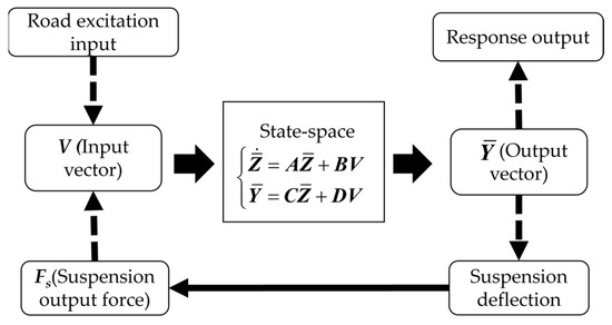
Figure 3.
Simulink simulation framework for solving the 14-DOF vehicle–cargo coupling model.
A numerical validation was conducted to ensure solution accuracy. The root mean square (RMS) acceleration of the vehicle floor under harmonic excitation served as the validation metric. Time integration employed the fourth-order Runge–Kutta scheme. To determine an appropriate time step, simulations were run with steps from 0.01 s down to 0.00125 s. The results indicated that step sizes of 0.0025 s or smaller kept RMS variations under 0.5%. Based on this finding, a step size of 0.0025 s was implemented. Convergence tests were performed across a range of relative tolerances, from 10−3 to 10−5. These tests showed that RMS variations remained below 0.1%. Consequently, the default relative tolerance in Simulink of 10−3 was retained.
3. Response Analysis
Assuming the road excitation follows a zero-mean isotropic Gaussian process, this study adopted the filtered white noise approach to generate Grade B (ISO 8608 [29]) road elevation profiles q1 to q4 as system inputs at a vehicle speed of 20 m·s−1 (72 km·h−1).
3.1. Verification of Model and Solution Approaches
In order to validate model accuracy and solution approaches, dynamic responses of air suspension vehicle were derived through Laplace transform and Simulink simulation. These simulated results were then benchmarked against collective vertical acceleration power spectral density (PSD) data from the vehicle floor from air suspension vehicles [30]. Figure 4 compares the PSDs from both solution approaches with this test data. Relevant parameters are detailed in the figure caption and Table 1, Table 2 and Table 3. The test data represent averaged acceleration PSD measurements from multiple air suspension trucks operating on diverse routes, demonstrating representative generality.
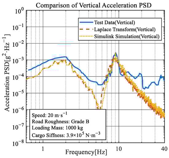
Figure 4.
Comparison of vertical acceleration PSD of vehicle floor.
As shown in Figure 4, results from both approaches demonstrate close agreement, validating the solution accuracy. Simulated and test data corresponded well in frequency and magnitude of the first two primary peaks in acceleration PSD, confirming the accuracy of coupling model. However, high-frequency peaks associated with vehicle frame structural modes were absent from the simulations due to modeling simplifications. Given the negligible discrepancy between the approaches, subsequent parameter analysis employed the Simulink simulation approach.
3.2. Effect of Orifice Resistance of Air Spring on Coupling Model
The influence of the orifice resistance (RF) on air spring stiffness characteristics was investigated. According to reference [12], values of RF = 0.5 × 10⁶ Pa·s·kg−1, 2.0 × 10⁶ Pa·s·kg−1, and 8.0 × 10⁶ Pa·s·kg−1 were selected, with other parameters listed in Table 3. According to reference [31], substituting s = iω into Equation (7), where ω denotes the angular frequency (rad·s−1), the dynamic stiffness Kair is expressed as follows:
where K1 and K2 denote storage stiffness and loss stiffness. Consequently, the magnitude ∣Kair∣ and phase angle φair are then given as follows:
Figure 5 shows the frequency-dependent stiffness under different RF. The results are plotted against cyclic frequency f (Hz), where the conversion ω = 2πf is implicitly applied. The air spring exhibits significant frequency dependence, demonstrating lower stiffness at low frequencies and higher stiffness at high frequencies. This characteristic aligns with the results presented in the literature [12,13]. Increased RF elevates gas flow impedance between chambers, causing systems with higher RF to reach high-stiffness plateaus more rapidly under rising excitation frequencies.
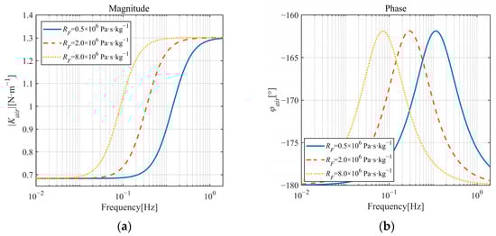
Figure 5.
The frequency-dependent stiffness of air springs under different RF: (a) Dynamic stiffness magnitude; (b) Dynamic stiffness phase.
System responses were computed under different orifice resistance (RF), with other parameters as specified in Table 1, Table 2 and Table 3. The resulting acceleration PSD responses for the vehicle floor and the two layers of cargo are shown in Figure 6, Figure 7 and Figure 8.
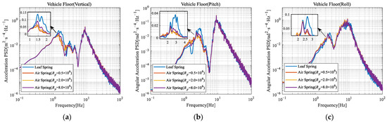
Figure 6.
Comparison of acceleration PSD of vehicle floor under different orifice resistance: (a) Vehicle floor (vertical); (b) Vehicle floor (pitch); (c) Vehicle floor (roll). [RF] = Pa·s·kg−1.
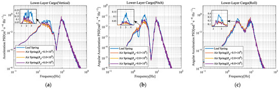
Figure 7.
Comparison of acceleration PSD of lower-layer cargo under different orifice resistance: (a) Lower-layer cargo (vertical); (b) Lower-layer cargo (pitch); (c) Lower-layer cargo (roll). [RF] = Pa·s·kg−1.
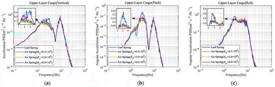
Figure 8.
Comparison of acceleration PSD of upper-layer cargo under different orifice resistance: (a) Upper-layer cargo (vertical); (b) Upper-layer cargo (Pitch); (c) Upper-layer cargo (roll). [RF] = Pa·s·kg−1.
Compared with the leaf spring suspension vehicle, the air suspension vehicle exhibited substantially lower magnitudes of the first peak (reduced by more than 50%) in vertical, pitch, and roll acceleration PSD. However, the magnitudes of the second peak were marginally higher (by approximately 10%). This reduction occurred because the frequency-dependent stiffness of air spring provides lower stiffness at low frequencies and higher stiffness at high frequencies. Consequently, the air suspension vehicle–cargo coupling model demonstrates softer suspension behavior in the low-frequency range, yielding smaller acceleration responses. Conversely, stiffer suspension characteristics in the high-frequency range produce larger acceleration responses.
Furthermore, increasing the orifice resistance elevates the suspension’s equivalent stiffness by modifying the air spring’s dynamic behavior. This increases the magnitude of first peak (within the suspension frequency band) in the acceleration PSD.
To quantitatively compare vibration reduction performance between suspension types, this study considered the relative vibration reduction effect (E) as follows:
where and denote the RMS values of the acceleration response for the leaf spring suspension vehicle and air suspension vehicle, respectively.
Figure 9 shows the relative vibration reduction effect (E) of the air suspension vehicles compared with the leaf spring suspension vehicles, with regard to the vehicle floor and two layers of cargo under different RF conditions. The error bars represent the standard deviation calculated from five independent random road excitation tests. The results demonstrate superior vibration reduction for air suspension in the vertical direction and pitch rotation. However, the air suspension exhibits comparatively inferior performance in roll rotation. This deficiency is attributed to its lower vertical stiffness, which consequently compromises roll stability. This finding aligns with previous research [21], which reported that softer suspensions reduce vibration but degrade roll stability. Furthermore, comparison of the relative vibration reduction effect (E) across cargo layers shows significantly reduced vibration in the upper layer in the vertical direction (14%) and pitch (28%) rotation.
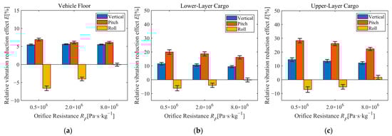
Figure 9.
Relative vibration reduction effect under different orifice resistance: (a) Vibration reduction (vehicle floor); (b) Vibration reduction (lower-layer cargo); (c) Vibration reduction (upper-layer cargo).
Comparative validation against published test data [32] confirmed the effectiveness of air suspension system used in this study. The vibration reduction effect (E) calculated from cargo vertical acceleration RMS measurements [32] ranges between 10–42%. The majority of simulated vertical vibration reduction effects (two layers of cargo) in Figure 9 fall within this range. Observed difference primarily may stem from simplifications in vehicle model and variations in cargo properties.
Figure 9 also illustrates the influence of RF on the relative vibration reduction effect. Increasing RF accelerates the transition of the air suspension to its high-frequency stiffness plateau. This stiffening elevates the effective roll stiffness, enhancing roll moment resistance and consequently improving E in the roll rotation. Conversely, the increased stiffness reduces E for vertical and pitch motions.
Therefore, adjustment of RF can optimize vertical vibration reduction performance. Since RF is related to orifice diameters, implementing variable orifice resistance in commercial freight vehicles is technically feasible. Engineers can actively control gas flow between the main and auxiliary air chambers using tunable orifices such as the mechanical multi-orifice valve that can be switched between predefined orifice diameters. This adjustment directly influences the air spring’s dynamic characteristics, optimizing vertical vibration reduction performance.
3.3. Effect of Loading Mass on Coupling Model
Simulations were conducted at three distinct truck loading levels: 20%, 60%, and 100% of the rated capacity. These correspond to total cargo masses of Mc = Mc1 + Mc2 = 1000 kg, 3000 kg, and 5000 kg, respectively. The rotational inertia of the cargo varied proportionally with the loading mass. For each loading condition, the rear suspension axle load was calculated through static equilibrium conditions, and the initial operating pressures of the air springs were subsequently determined based on these calculated loads. Table 4 presents the resulting initial air spring pressures for the air suspension vehicle under different loading mass.
Table 4.
Initial operating pressure of air spring under different loading mass.
The initial air spring operating pressures were set according to loading mass, while other parameters (excluding loading mass and cargo rotational inertia) remained consistent with Table 1, Table 2 and Table 3. Consequently, the system responses under the different loading mass conditions were computed. As this study concentrates on the influence of the air suspension on cargo dynamics, subsequent analyses focus exclusively on cargo responses.
Figure 10 and Figure 11 compare cargo acceleration PSD under different loading mass. As the total cargo mass increases, both mass and rotational inertia increase while cargo stiffness remains unchanged. This reduces the natural frequencies of vibration modes dominated by cargo, shifting the first peak toward lower frequencies across all response PSD. The following key trends were also observed in the cargo responses:
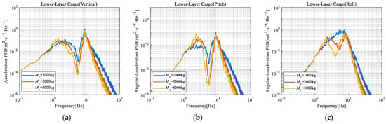
Figure 10.
Comparison of acceleration PSD of lower-layer cargo under different loading mass: (a) Lower-layer cargo (vertical); (b) Lower-layer cargo (pitch); (c) Lower-layer cargo (roll).
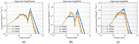
Figure 11.
Comparison of acceleration PSD of upper-layer cargo under different loading mass: (a) Upper-layer cargo (vertical); (b) Upper-layer cargo (pitch); (c) Upper-layer cargo (roll).
- Vertical Response PSD: The increasing mass reduces the magnitude of second peak, particularly for upper-layer cargo where reductions exceed 95%. The attenuation of the second peak might be attributed to reduced acceleration resulting from increased mass under equivalent excitation forces;
- Pitch Response PSD: As loading mass increases, the magnitude of the first peak rises. Conversely, the magnitude of the second peak decreases, exhibiting a pronounced reduction for the upper-layer cargo. The first peak amplification may result from mass-induced modal frequency shift, concentrating vibrational energy within specific bands. The second peak attenuation may result from the reduction in acceleration due to increased mass under equivalent excitation;
- Roll Response PSD: Peak coalescence is observed in the roll response at the lowest loading mass level. This phenomenon may originate from mass-induced modal frequency shift in the vehicle–cargo coupling model.
3.4. Effect of Cargo Stiffness on Coupling Model
In this study, the cargo stiffness is defined as the equivalent stiffness derived from the compression displacement of the cargo cushion under static loading. In agreement with the literature [26], the cargo cushion compression displacements were set to 2 cm, 3 cm, and 4 cm under a static load of 5000 kg. The corresponding distributed stiffness coefficient of the cargo (Kc = Kc1 = Kc2) were calculated as 3.90 × 10⁵ N·m−3, 2.60 × 10⁵ N·m−3, and 1.95 × 10⁵ N·m−3. A constant cargo damping ratio of 0.1 was maintained across all configurations. Additional parameters are detailed in Table 1, Table 2 and Table 3. The acceleration PSD responses of the cargo for these stiffness conditions are presented in Figure 12 and Figure 13.
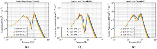
Figure 12.
Comparison of acceleration PSD of lower-layer cargo under different cargo stiffness: (a) Lower-layer cargo (vertical); (b) Lower-layer cargo (pitch); (c) Lower-layer cargo (roll).
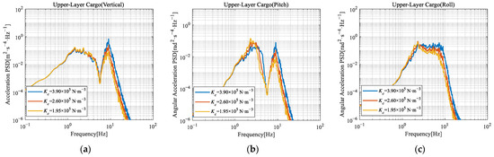
Figure 13.
Comparison of acceleration PSD of upper-layer cargo under different cargo stiffness: (a) Upper-layer cargo (vertical); (b) Upper-layer cargo (pitch); (c) Upper-layer cargo (roll).
Analysis reveals that reducing cargo stiffness from 3.90 × 10⁵ N·m−3 to 1.95 × 10⁵ N·m−3 at constant mass lowers the natural frequencies of vibration modes dominated by cargo, thereby shifting the first peak of PSD toward lower frequencies. The following other key response trends were observed:
- Vertical Response PSD: The stiffness reduction primarily affects the second peak of PSD (upper-layer cargo), reducing its magnitude by up to 87%. This magnitude reduction is likely associated with depressed modal stiffness. Overall, decreased stiffness correlates with reduced vibration intensity, aligning with previous findings [26];
- Pitch Response PSD: The magnitude of the first peak increases, while the second peak magnitude decreases significantly for upper-layer cargo. This phenomenon stems from system modal restructuring due to the reduction of cargo stiffness;
- Roll Response PSD: Similarly, the stiffness reduction primarily attenuates the second peak, particularly for upper-layer cargo. This reduction results from modal restructuring due to the changing stiffness.
Overall, the reduction of cargo stiffness exhibits a more pronounced effect on the upper-layer cargo. This heightened sensitivity is likely due to its position within the cargo stack.
4. Conclusions and Discussion
This study investigates the dynamic response of a vehicle–cargo coupling model, explicitly accounting for the frequency-dependent stiffness characteristics in air suspension. Key findings are summarized as follows:
- Compared with vehicles equipped with leaf spring suspensions, air suspension vehicles exhibit a significant magnitude reduction (>50%) of the first peak in acceleration PSD. Although the magnitude of second peak increases by approximately 10%, the overall vibration attenuation performance of air suspensions remains superior;
- Replacing the leaf spring suspension with an air suspension significantly improves vibration suppression in upper-layer cargo (14% vertical, 28% pitch reduction) compared with lower-layer cargo under identical parameters. However, cargo roll angles should be controlled to prevent potential overturning incidents;
- Parametric studies reveal that increased orifice resistance directly influences the frequency-dependent stiffness of the suspension, amplifying its high-frequency stiffening characteristics. This leads to elevated magnitude of the first peak in PSD and an overall increase in system response. Increased loading mass or reduced cargo stiffness shift peaks in PSD toward lower frequencies, attenuating the second peak of PSD. Upper-layer cargo exhibits higher sensitivity to parameter variations. Consequently, light loading conditions significantly amplify the vertical vibrations of upper-layer cargo. This can be mitigated by combining low-stiffness cushioning materials with tunable valve control to reduce orifice resistance (RF), effectively suppressing distinct frequency-domain resonance peaks.
These findings provide practical guidelines for designing cargo transportation schemes in air suspension vehicles to enhance cargo safety. The following three major limitations in this study can be addressed in future research:
- The model assumes small displacement amplitudes, restricting its applicability to nonlinear regimes involving large suspension travels;
- This study employed stationary Gaussian random road signals, whereas actual road profiles exhibit non-Gaussian characteristics with transient impacts;
- The current model specifically applies to two-axle vehicles. Extensions to tri-axle trucks or tractor-trailers require dedicated modeling frameworks due to their fundamentally distinct structural configurations.
Author Contributions
Conceptualization, Z.-W.W. and Y.-T.Z.; methodology, Z.-W.W. and Y.-T.Z.; software, Y.-T.Z.; validation, Y.-T.Z.; writing original draft preparation, Y.-T.Z.; writing—review and editing, Z.-W.W. and Y.-T.Z.; supervision, Z.-W.W.; funding acquisition, Z.-W.W. All authors have read and agreed to the published version of the manuscript.
Funding
This research was funded by National Natural Science Foundation of China (No. 50775100).
Institutional Review Board Statement
Not applicable.
Informed Consent Statement
Not applicable.
Data Availability Statement
The original contributions presented in the study are included in the article. Further inquiries can be directed to the corresponding author.
Acknowledgments
DeepSeek-R1 was employed during the preparation of this manuscript for language polishing and refinement. The authors have thoroughly reviewed and edited the AI-generated content and take full responsibility for the content of this publication.
Conflicts of Interest
The authors declare no conflicts of interest.
Abbreviations
The following abbreviations are used in this manuscript:
| MDOF | Multi-degree-of-freedom |
| 14-DOF | 14-degree-of-freedom |
| CM | Center of mass |
| PSD | Power spectral density |
| RMS | Root mean square |
Appendix A
References
- Agarwal, A.; Mthembu, L. Design and response surface optimization of heavy motor vehicle chassis using P100/6061 Al MMC. In Recent Advances in Materials and Modern Manufacturing: Select Proceedings of ICAMMM 2021; Springer Nature: Singapore, 2022; pp. 1–12. [Google Scholar]
- Issa, M.; Samn, A. Passive vehicle suspension system optimization using Harris Hawk Optimization algorithm. Math. Comput. Simul. 2022, 191, 328–345. [Google Scholar] [CrossRef]
- Ding, X.; Wang, Z.; Zhang, L.; Liu, J. A comprehensive vehicle stability assessment system based on enabling tire force estimation. IEEE Trans. Veh. Technol. 2022, 71, 11571–11588. [Google Scholar] [CrossRef]
- Zhou, R.; Zhang, B.; Li, Z. Dynamic modeling and computer simulation analysis of the air spring suspension. J. Mech. Sci. Technol. 2022, 36, 1719–1727. [Google Scholar] [CrossRef]
- Gavriloski, V.; Jovanova, J.; Tasevski, G.; Djidrov, M. Development of a new air spring dynamic model. FME Trans. 2014, 42, 305–310. [Google Scholar] [CrossRef]
- Wu, M.Y.; Yin, H.; Li, X.B.; Lv, J.C.; Liang, G.Q.; Wei, Y.T. A new dynamic stiffness model with hysteresis of air springs based on thermodynamics. J. Sound Vib. 2022, 521, 116693. [Google Scholar] [CrossRef]
- Zhu, H.; Yang, J.; Zhang, Y.; Feng, X. A novel air spring dynamic model with pneumatic thermodynamics, effective friction and viscoelastic damping. J. Sound Vib. 2017, 408, 87–104. [Google Scholar] [CrossRef]
- Mendia-Garcia, I.; Facchinetti, A.; Bruni, S.; Gil-Negrete, N. Analysis and modelling of the dynamic stiffness up to 400 Hz of an air spring with a pipeline connected to a reservoir. J. Sound Vib. 2023, 557, 117740. [Google Scholar] [CrossRef]
- Shi, Y.; Xu, S.F.; Li, Z.L.; Nie, Y.; Sun, Z. Dynamic frequency response characteristics of a compound regulative quasi-zero stiffness air spring system. Sci. China Technol. Sci. 2023, 66, 2013–2024. [Google Scholar] [CrossRef]
- Locken, F.; Welsch, M. The dynamic characteristic and hysteresis effect of an air spring. Int. J. Appl. Mech. Eng. 2015, 20, 127–145. [Google Scholar] [CrossRef]
- Li, Y.; Xiao, S.; Xie, J.; Zhu, T.; Zhang, J. Nonlinear dynamic mechanical characteristics of air springs based on a fluid–solid coupling simulation method. Appl. Sci. 2023, 13, 12677. [Google Scholar] [CrossRef]
- Quaglia, G.; Sorli, M. Air suspension dimensionless analysis and design procedure. Veh. Syst. Dyn. 2001, 35, 443–475. [Google Scholar] [CrossRef]
- Nieto, A.J.; Morales, A.L.; Gonzalez, A.; Chicharro, J.M.; Pintado, P. An analytical model of pneumatic suspensions based on an experimental characterization. J. Sound Vib. 2008, 313, 290–307. [Google Scholar] [CrossRef]
- Chen, Y.; Peterson, A.W.; Ahmadian, M. Achieving anti-roll bar effect through air management in commercial vehicle pneumatic suspensions. Veh. Syst. Dyn. 2019, 57, 1775–1794. [Google Scholar] [CrossRef]
- Li, H.; Li, S.; Sun, W.; Wang, L.; Lv, D. The optimum matching control and dynamic analysis for air suspension of multi-axle vehicles with anti-roll hydraulically interconnected system. Mech. Syst. Signal Process. 2020, 139, 106605. [Google Scholar] [CrossRef]
- Bai, X.; Lu, L.; Zhang, C.; Geng, W. Research on height adjustment characteristics of heavy vehicle active air suspension based on fuzzy control. World Electr. Veh. J. 2023, 14, 210. [Google Scholar] [CrossRef]
- Van, L.V.; Tung, N.T. Application of air suspension system on multi-purpose forest fire fighting vehicle for reducing dynamic load. J. Vib. Eng. Technol. 2024, 12, 7219–7230. [Google Scholar] [CrossRef]
- Moheyeldein, M.M.; Abd-El-Tawwab, A.M.; Abd El-Gwwad, K.A.; Salem, M.M.M. An analytical study of the performance indices of air spring suspensions over the passive suspension. Beni-Suef Univ. J. Basic Appl. Sci. 2018, 7, 525–534. [Google Scholar] [CrossRef]
- Le, V.Q. Comparing the performance of suspension system of semi-trailer truck with two air suspension systems. Vibroengineering Procedia 2017, 14, 220–226. [Google Scholar] [CrossRef]
- Guowei, D.; Wenhao, Y.; Zhongxing, L.; Khajepour, A.; Senqi, T. Sliding mode control of laterally interconnected air suspensions. Appl. Sci. 2020, 10, 4320. [Google Scholar] [CrossRef]
- Zhu, H.; Yang, J.; Zhang, Y. Dual-chamber pneumatically interconnected suspension: Modeling and theoretical analysis. Mech. Syst. Signal Process. 2021, 147, 107125. [Google Scholar] [CrossRef]
- Bernad, C.; Laspalas, A.; González, D.; Liarte, E.; Jiménez, M.A. Dynamic study of stacked packaging units by operational modal analysis. Packag. Technol. Sci. Int. J. 2010, 23, 121–133. [Google Scholar] [CrossRef]
- Wang, Z.W.; Wang, L.J. Accelerated random vibration testing of transport packaging system based on acceleration PSD. Packag. Technol. Sci. 2017, 30, 621–643. [Google Scholar] [CrossRef]
- Keyhan, S.; Shirzad, K.; Almenar, E.; Joodaky, A. Transportation Vibration Effects on Apple Bruising. Packag. Technol. Sci. 2024, 37, 1065–1071. [Google Scholar] [CrossRef]
- Wang, Z.W.; Zhong, L.L. Finite element analysis and experimental investigation of beer bottle turnover boxes transport unit under random vibration excitation. Packag. Technol. Sci. 2020, 33, 197–214. [Google Scholar] [CrossRef]
- Huang, M.Q.; Wang, Z.W. Response analysis of transportation system based on vehicle-cargo coupling. J. Vib. Eng. 2024, 37, 1906–1916. [Google Scholar]
- Molnár, B.; Böröcz, P. Experimental comparison of field and accelerated random vertical vibration levels of stacked packages for small parcel delivery shipments. Appl. Sci. 2021, 11, 2927. [Google Scholar] [CrossRef]
- ISO 6358-1:2013; Pneumatic Fluid Power-Determination of Flowrate Characteristics of Components Using Compressible Fluids. Part 1: General Rules and Test Methods for SteadyState Flow. ISO: Geneva, Switzerland, 2013.
- ISO 8608:2016; Mechanical Vibration-Road Surface Profiles-Reporting of Measured Data. ISO: Geneva, Switzerland, 2016.
- Singh, J.; Singh, S.P.; Joneson, E. Measurement and analysis of US truck vibration for leaf spring and air ride suspensions, and development of tests to simulate these conditions. Packag. Technol. Sci. Int. J. 2006, 19, 309–323. [Google Scholar] [CrossRef]
- Zheng, Y.; Shangguan, W.B. A combined analytical model for orifice-type and pipe-type air springs with auxiliary chambers in dynamic characteristic prediction. Mech. Syst. Signal Process. 2023, 185, 109830. [Google Scholar] [CrossRef]
- Soleimani, B.; Ahmadi, E. Measurement and analysis of truck vibration levels as a function of packages locations in truck bed and suspension. Comput. Electron. Agric. 2014, 109, 141–147. [Google Scholar] [CrossRef]
Disclaimer/Publisher’s Note: The statements, opinions and data contained in all publications are solely those of the individual author(s) and contributor(s) and not of MDPI and/or the editor(s). MDPI and/or the editor(s) disclaim responsibility for any injury to people or property resulting from any ideas, methods, instructions or products referred to in the content. |
© 2025 by the authors. Licensee MDPI, Basel, Switzerland. This article is an open access article distributed under the terms and conditions of the Creative Commons Attribution (CC BY) license (https://creativecommons.org/licenses/by/4.0/).