Abstract
The manufacturing of multiscale composite structures in aerospace engineering is governed by complex interactions among material heterogeneity, fluid rheology, and multiphysics phenomena—including thermal, chemical, electrical, and mechanical effects. These coupled processes introduce significant challenges during both processing and post-manufacturing stages, which are often difficult to resolve using traditional (experimental) trial-and-error approaches. This review explores the potential of advanced numerical methods and simulation frameworks to address these complexities. Emphasis is placed on the use of finite element and finite volume methods, along with their respective solution strategies and domain discretisation techniques, to solve the coupled governing equations involved in composite manufacturing processes. By integrating theory, computation, and physics-based understanding, these approaches enable predictive capability and design optimisation in the development of high-performance composite components for aerospace applications; many challenges though still remain in fabrication, design, and analysis.
1. Introduction
Numerical means continue to have potential for parameter predictions in a diverse range of engineering applications such as energy, marine, automotive, and aerospace. With applications in aerospace structures, the design and manufacturing of composites are vital when considering high strength–weight ratio, light weight, durability, shape flexibility, and chemical resistance [1]. Such composites consist of two or more materials combined together prior to the manufacturing phase. These materials, generally, are classified into two main parts—matrices and reinforcements. This review will examine numerical works on the use of thermoset polymers (e.g., epoxy, polyester) and synthetic/natural fibres (e.g., carbon) as composite matrices and reinforcements, respectively. The aforementioned combination has received much attention within aerospace industries for its pivotal role in substituting metal-based parts, cost-cutting, and continuously improving efficiency. The good news is that manufacturing processes, as well as the post-manufacturing tests of fibre-reinforced polymer composites (FRPCs), can now be modelled and simulated by a variety of accurate and reliable numerical techniques. The finite element method (FEM) and finite volume method (FVM) are some of the more widely used techniques that allow the transformation (conversion) of partial differential equations (PDEs), such as the Navier–Stokes equations (for flow), into an algebraic form that can be numerically solved throughout a discretised domain—see Figure 1. Other methods include the finite difference method (FDM) [2,3] and lattice Boltzmann method (LBM) [4,5,6]; however, the FDM is restricted to structured mesh (regular grids), andthe LBM is a memory-consuming algorithm and is limited to specific flow regimes. It should be noted that the aforementioned methods are applicable to flow problems. The FEM can also be used to simulate the behaviour of objects when subjected to stresses and strains (loads and boundary conditions); similarly, the so-called boundary element method (BEM)—analysing only boundary elements of the domain—is another promising numerical solution for structural analysis [7]. AI applications in composite manufacturing, particularly machine learning and deep learning, could help reduce analysis time and predict material properties [8,9]. The integration of machine learning with multiscale FEM and FVM frameworks is transforming how composite manufacturing processes—such as permeability prediction, curing, and residual stress analysis—are modelled. Karuppusamy et al. [9] highlight the use of supervised learning models, such as artificial neural networks and support vector machines, for predicting key composite properties based on fibre–matrix interactions and processing parameters. These models reduce the computational cost of traditional simulations and enhance insight into process–structure–property relationships. Similarly, Wu et al. [10] developed gated recurrent unit (GRU) surrogates embedded into FEM multiscale workflows to approximate meso-scale mechanical behaviour, achieving significant speed improvements for tasks like resin impregnation modelling. Furthermore, Yang et al. [11] demonstrated how convolutional neural networks (CNNs) trained on FEM-generated microstructure–response data can accurately predict stress fields, enabling defect-aware property mapping without repeated simulations. Collectively, these hybrid AI–physics models provide a scalable, efficient solution to modelling the complex, nonlinear, and path-dependent behaviour of composites across manufacturing scales. However, this still requires both the quantity and quality of data, which remain areas of active research and development [12]. Figure 2 illustrates the hierarchical architecture of fibre-reinforced composites, highlighting the transition from micro-scale fibre–matrix interactions to the macro-scale laminate structure. This inherent multiscale complexity introduces major challenges in modelling and simulation, particularly in capturing properties such as permeability, cure kinetics, and local stress distributions. A key issue is how to effectively transfer information across scales—for instance, employing representative volume elements (RVEs) at the micro-scale to estimate macroscopic permeability or using meso-scale woven models to inform laminate-level behaviour. In some cases, macro-scale process data may also be used to infer micro-scale conditions, enabling inverse estimation of internal fields. Addressing these scale-bridging challenges is essential for accurate and predictive modelling of composite manufacturing processes.
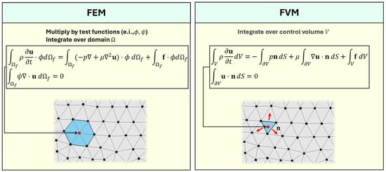
Figure 1.
Schematic comparison between the finite element method (FEM) and the finite volume method (FVM) for solving governing equations in computational fluid dynamics (CFD). In the FEM (left), the equations are weighted by test functions (e.g., , ) and integrated over the entire computational fluid domain , resulting in a weak formulation suitable for unstructured meshes and higher-order approximations. The highlighted region illustrates an element-centred discretisation approach. In contrast, the FVM (right) is based on the integral form of the governing equations over discrete control volumes V, ensuring local conservation by evaluating fluxes across control surfaces . The diagram illustrates a control volume, with surface normals n indicating flux directions across the cell.
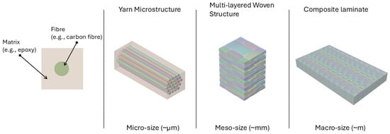
Figure 2.
Hierarchical structure of polymer-based composites shown across different length scales: fibre held within a matrix (micro-scale), yarn microstructure, multi-layered woven structure (meso-scale), and the final composite laminate (macro-scale).
This review provides insights into numerical works based on FVM and FEM for flow analyses, and FEM for structural problems. Studies on coupled (twining) approaches—fluid structural interfaces (FSIs)—are also raised. Discretisation methods and calculation approaches for PDEs are thoroughly discussed.
2. FEM in Composite Manufacturing
2.1. FEM: Governing PDEs to Algebraic Form
In this subsection, an illustrative brief example is given for a unsteady incompressible Newtonian fluid (i.e., Stokes flow), usually the case for resin moulding of composites (impregnation of fibre preforms), to demonstrate the FEM numerical solution of a CFD (flow) problem [13,14,15,16]. This usually starts with partial differential equations (PDEs) of a governing equation (e.g., Stokes flow)—see Equations (1) and (2) below:
where is the pressure gradient, is the viscous term, and is the source term. Then, a weak/variational form is applied to integrate the PDEs over the fluid domain () using test/basis functions (, ).
This allows the integration of the PDEs to attain a saddle-point matrix (i.e., algebraic form/system).
where and are matrices, while and are gradient and divergence operators, respectively. and are vectors of unknown nodal velocity and pressure, and is the body force or source term vector. is a time step size, while n and indicate the current time level and next/future time level, respectively.
2.2. Review of FEM-Based Numerical Studies
The FEM has been and still is applied in composite manufacturing as a prediction and optimisation tool to characterise parameters like permeability, porosity, tortuosity, curing, etc. For instance, Tan et al. [17] used the FEM approach to predict resin flow progression in a dual-scale porous media during an RTM process. A PoreFlow, based on a Fortran modular package, was utilised to run the FEM numerical calculations. This was to predict two-scale permeability, macro and micro, in an effort to waive the use of fitting parameters as well as to optimise the infiltration of resin into the fibrous preforms, void formation, and reverse flow. The authors [17] validated FEM-based results with available experimental data, which manifested its capability to simulate liquid moulding of composites—see Figure 3. Likewise, a study by Simacek et al. [18] adopted an FEM approach using LIMS (Liquid Injection Moulding Simulation) software to account for capillary effects within the fibre tow scale for resin impregnation modelling. The authors [18] revealed that capillarity can slow intra-tow filling and, consequently, leave voids or dry spots at the micro-level. The study emphasised the model’s reliability in such advanced transport phenomena (capillary effect inclusion) via validation against experimental data. Oliveira et al. [19] applied the FEM approach, implemented in PAM-RTM software, to perform macro-scale flow simulations (i.e., overall permeability prediction). The study [19] validated the FEM-based PAM-RTM results of flow-front progression against experimental flow behaviour in the mould, manifesting its feasibility. Dealing with curing, a study by Cheung et al. [20] addressed such phenomena using the FEM implemented in commercial Apaqus software. This was used to couple transient heat conduction with resin cure reaction (an autocatalytic model) to capture the evolution of resin temperature and degree of cure during exothermic heat generation. The FEM-based simulations were validated against experimental data—literature benchmarks—for temperature distribution and cure degree profiles. Yet another work by Sandberg et al. [21] studied the resin flow, heat transfer, and cure kinetics of a thermosetting system (polyurethane resin) in the pultrusion process, as shown in Figure 4, using FEM-based COMSOL multiphysics 5.4 software. The authors [21] compared simulated temperature and degree-of-cure profiles with available measured data from pultrusion experiments, by which a good agreement was reached, validating the developed numerical model for use in composite manufacturing analysis. Table 1 highlights key FEM-based numerical studies focused on simulating composite manufacturing processes.
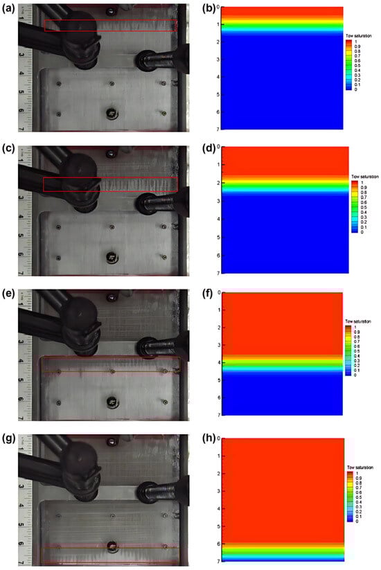
Figure 3.
Experimental and simulated flow-front progression during isothermal resin impregnation of a unidirectional fibre preform under constant pressure conditions. (a,c,e,g) show visual flow-front images captured at successive time steps. (b,d,f,h) show the corresponding numerical tow saturation contours. The colour scale indicates local saturation ranging from 0 (unsaturated) to 1 (fully saturated). These results illustrate the transient infiltration behaviour and validate the model’s ability to capture intra-tow and inter-tow flow dynamics [17].
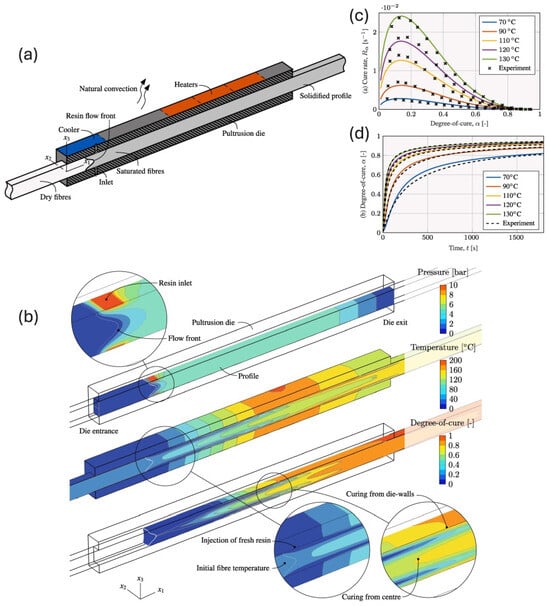
Figure 4.
Simulation results and experimental validation of a reactive pultrusion process, showing resin pressure, temperature, and degree of cure evolution along a 3D pultrusion die—(a). Left (b): Distribution of pressure (top), temperature (middle), and degree of cure (bottom) along the die, including detailed insets showing the flow-front progression and localised curing patterns from the die-walls and centre. Right: (c) Predicted cure rate versus degree of cure for various temperatures, compared with experimental data. (d) Predicted degree of cure versus time for the same temperature set, with validation against experimental measurements [21].

Table 1.
Selected numerical contributions evaluating FEM-based tools for modelling composite manufacturing processes.
FEM-based tools such as Poreflow, LIMS, PAM-RTM, and COMSOL are widely used for modelling resin flow in fibrous porous media. Poreflow and LIMS excel in permeability-focused RTM simulations, PAM-RTM is valued in industry for robust process prediction, and COMSOL offers multiphysics flexibility for integrating flow, heat transfer, and cure kinetics. Ultimately, selecting the most suitable platform depends on the modelling objectives, whether the priority is process-specific simulation or multiphysics integration.
To sum up, the FEM is well-known for its strong multiphysics coupling, integrating flow, heat transfer, chemical reactions, and structural responses within a single solver framework. The literature shows accurate flow-front tracking using this method, via Level Set approach, which effectively captures the evolution of interfaces or moving fronts. Additionally, the FEM offers great adaptability to unstructured meshes and complex geometries. However, it remains computationally intensive when simulating transient (unsteady) flows. Further work is also needed to stabilise solutions in convection-dominated regimes and to reduce numerical oscillations (errors). Overall, the FEM is preferred when detailed coupling of structural, thermal, and chemical phenomena is required.
3. FVM in Composite Manufacturing
3.1. FVM: Governing PDEs to Algebraic Form
Like the FEM, the FVM starts with the strong PDE form of the momentum and continuity equations—Stokes Equations (1) and (2), as mentioned earlier in Section 2.1 [22,23,24,25]. Instead of multiplying the PDE by test functions (like in FEM) over the domain, the FVM integrates the PDE over each control volume (cell), and uses the divergence theorem (Gauss’s theorem) to covert the control volume to surface integrals—see Equations (6) and (7).
Thereby, this leads to an algebraic form (see Equations (8) and (9)) that is appropriate for numerical calculations—typically solved using iterative schemes like SIMPLE (Semi-Implicit Method for Pressure-Linked Equations).
where is a matrix that combines transient and viscous terms, and stand for the pressure-gradient operator and divergence operator, respectively, and here includes previous time step velocity and body forces.
3.2. Review of FVM-Based Numerical Studies
The use of the FVM may be preferred to the FEM for CFD problems due to its simplicity on arbitrary meshes (e.g., tetrahedrons) and no requirement for basis or test functions—direct flux calculations. A work by Grössing et al. [26], based on the FVM, uses OpenFoam (i.e., open-source CFD) to characterise resin flow advancement in dual-scale porous medium. The FVM-based OpenFoam capability was attested in capturing unsaturated permeabilities as it agreed well with the flow-front experimental data—see Figure 5. A study by Alotaibi et al. [27] utilised ANSYS Fluent 19.2 (FVM solver) to calculate Stokes–Brinkman equations (micro–meso-scale simulation) with consideration of the yarn curvature effect on resin flow. The source term, provided in the momentum Equation, was employed for micro-permeability (intra-tow pores) while the Stokes equation (remaining terms) was applied for inter-tow pores. The numerical analysis [27] promoted the reliability of the FVM used in Fluent, and the ability to adopt a more customised flow problem—curvature/waviness impact. Wei et al. [28] adopted the FVM using the Moldex3D tool to describe the behaviour of resin flow in fibre preforms. The authors [28] concluded that the FVM-based flow-front simulations indicated consistency with the data from infusion experiments, and thus an estimation of the permeability/porosity ratio was obtained as a means to stabilise flow front in the mould. With respect to the curing of polymer composites, the work by Alotaibi et al. [29] managed to couple filling and curing simulations, using FVM-based Fluent, by incorporating customised codes into the commercial code for heat generation, viscosity evolution, and degree of cure. The coupled numerical approach was verified with the literature, and also demonstrated its capability to accurately simulate resin flows under varying process conditions (e.g., ability to predict early cure, notably during the fill stage, as can be seen in Figure 6), employing high-order upwinding interpolation schemes to enhance stability and convergence. A similar study by Yang et al. [30] used FVM-based Fluent to optimise the cure cycle (during cure stage) with the aim of achieving uniformity in cure, besides avoiding residual stresses. The numerical method was eventually validated with temperature development profiles, see Figure 7, in a resin transfer moulding (RTM) experiment. Wittemann et al. [31] analysed curing behaviour by integrating viscosity and cure models into a CFD code using OpenFoam—FVM solver. The study [31] modelled thermosets in reinforced reactive injection moulding (RRIM), whereby the FVM-based calculations matched well with experimental pressure measurements over the filling stage, showing the method’s high potential. An overview of representative FVM-based modelling efforts applied to composite manufacturing is presented in Table 2.
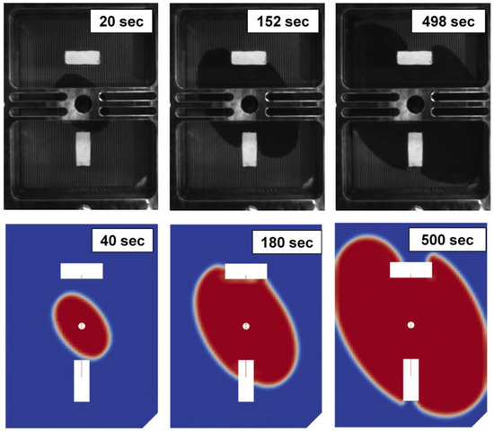
Figure 5.
Comparison of experimental (top) and simulation (bottom) results showing resin flow in a mould over time. The resin front progresses at different time steps, showing good agreement between the experiment and the numerical model [26].
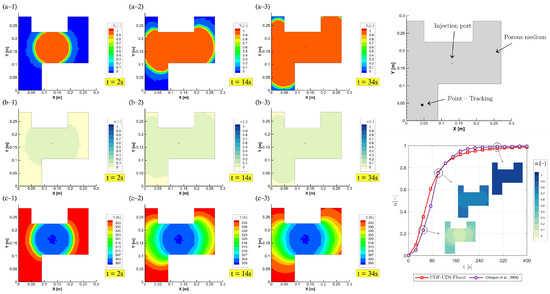
Figure 6.
Numerical simulation of resin flow, curing, and temperature distribution during the resin transfer moulding (RTM) process in a porous medium with a complex cavity shape. Sub-figures (a-1–a-3) depict the evolution of resin volume fraction at 2 s, 14 s, and 34 s, respectively. Sub-figures (b-1–b-3) show the corresponding distribution of the degree of cure , while sub-figures (c-1–c-3) illustrate the transient temperature fields in Kelvin. The top-right diagram indicates the location of the injection port, porous medium, and point-tracking position used for monitoring the curing behaviour. The bottom-right plot compares the degree of cure over time at the tracking point between the current UDF-UDS Fluent model and reference results from the literature, demonstrating strong agreement [29,32].
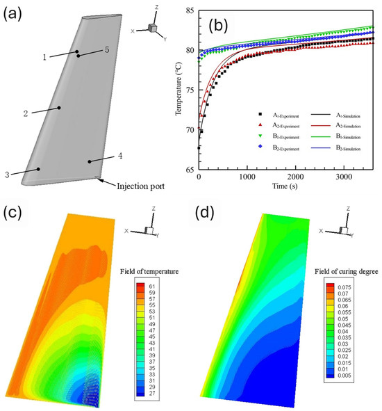
Figure 7.
Simulation and experimental validation of temperature and cure behaviour in a composite part during the resin transfer moulding (RTM) process. Top-left (a): 3D schematic of the part showing the injection port and five measurement points for temperature monitoring. Top-right (b): Comparison between experimental and simulated temperature histories at different locations (1, 2, 3, 4, 5), demonstrating good agreement across all positions. Bottom-left (c): Simulated temperature field within the part at a representative curing stage. Bottom-right (d): Corresponding field of degree of cure, showing the distribution of the curing progression throughout the part [30].
Table 2.
Selected numerical contributions evaluating FVM-based tools for modelling composite manufacturing processes.
Among the main FVM-based tools used to model resin flow in fibrous porous media, OpenFOAM, ANSYS Fluent, and Moldex3D are the most commonly applied. OpenFOAM is popular in research because it is open-source and allows users to fully customise the simulation to include important physical effects like Darcy’s law. ANSYS Fluent is a commercial tool known for its reliable results and flexibility through user-defined functions, which help model complex behaviours such as resin curing and variable viscosity. Moldex3D is often used in industry, especially for thermoplastic composites, because it is easy to use and includes built-in features for mould filling and porous flow. Overall, OpenFOAM and Fluent are preferred for more detailed and accurate simulations, while Moldex3D is chosen when ease of use and process integration are more important.
In summary, the finite volume method (FVM) is well-suited for large-scale computational fluid dynamics (CFD) problems, offering strong parallel scalability and computational efficiency. However, it has limitations in structural integration, as the finite element method (FEM) is still required to model the mechanical response. Additionally, incorporating cure kinetics or micro-scale permeability effects often requires customisation of the governing PDEs, typically through user-defined functions (UDFs). Overall, this numerical approach is generally preferred when simulation scalability is of great importance.
4. Multiphysics Coupling: Fluid, Thermo-Chemical, and Structural Domains
4.1. Coupling Hypothesis
A detailed linkage equation via coupling or the so-called digital twinning (interaction) between fluid (liquid resin) and structure (fibre tows) is given within this Section by an illustrative numerical approach for residual stresses [33,34,35,36]—see Figure 8 for more insight.
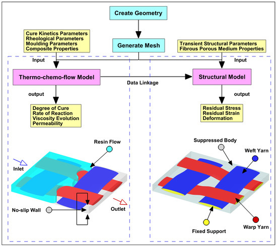
Figure 8.
Integrated simulation framework for predicting the thermo-chemo-mechanical behaviour of woven composite laminates during resin transfer moulding (RTM). The workflow begins with geometry creation and mesh generation, followed by two coupled models: the thermo-chemo-flow model (left), which takes input parameters such as cure kinetics, rheology, and moulding conditions to compute outputs including degree of cure, reaction rate, viscosity evolution, and permeability; and the structural model (right), which incorporates transient structural and fibrous medium properties to evaluate residual stress, strain, and deformation. Data linkage between the two models ensures coupling of thermal–chemical and mechanical behaviour. Bottom visualisations show the simulation setup, including resin flow domain and structural constraints applied to the woven yarn architecture [37].
These residual stresses are usually the remaining internal stresses after applying a force/load. This load can be induced by flow, heat (e.g., thermal expansion), or reaction (e.g., cure shrinkage). In this manner, Von Mises theory is used by the structure side (explained within this Section), while the fluid and/or thermo-chemical side is governed by unsteady incompressible Newtonian Stokes equations along with energy and species transport equations—the methodology is outlined in greater detail in Appendix A.
Here, is a structural displacement vector, is the stress tensor, and is the solid domain. Pressure p and velocity are computed from the fluid side to provide traction () at the interface (), likewise for temperature —see Equations (10) and (11). This traction will act as an external force (load) on a body. Based on this premise, displacements (deformation) can be caused at the solid (structure) side, and from that deformation, strains and stresses can be evaluated. Following the results of the stress tensor () in Equation (12), Von Mises stress (), from Equation (13), is calculated to map residual stresses throughout the structure body, in particular fibre tows.
4.2. Review of Numerical Studies on Multiphysics Coupling
In fluid–structure interaction (FSI) simulations, the FEM is mainly used in the solid domain, while the FVM or FEM may be used in the fluid domain. Such linkage (transient fluid to structural response) is already discussed within Section 4.1. Reviews on structural response to loads caused by resin flow or cure are discussed within this Section. Yuan et al. [38] used Abaqus coupled with UMATHT and USEFLD (user subroutines) to link thermal/chemical effects during the curing process of composite materials. This was to predict macro-scale simulations of temperature, and degree of cure at the part level, as a means to use the aforementioned results for calculating micro-stresses (residual stresses) at fibre level. The proposed twinning method (thoroughly FEM-based) was validated with temperature data obtained from the literature, as illustrated in Figure 9, suggesting that micro-stresses occur at both the fibre and polymer (matrix) sides due to thermal expansion and curing shrinkage. A study by Alotaibi et al. [37] performed fluid–solid coupling simulations using FVM-FEM linkage—Fluent+ANSYS-Mechanical—to characterise residual stresses of fibre structures at the meso-micro-level. The fluid–solid coupling included effects of flow-induced load/deformation, thermally induced expansion, and cure-induced shrinkage during the two stages: filling and curing. The developed model had the potential to twin the FVM-based convection–reaction–diffusion flow (resin) problem with the FEM-based structural (carbon fibre) response for the interpretation of deformation, and residual stresses or strains in fibre preforms. Goncalves et al. [39] investigated the development of micro-residual stresses in carbon/epoxy polymer composites during the curing process using numerical simulation. The authors [39], similar to [38], employed the commercial FEM software Abaqus with user subroutines to account for thermal, chemical, and mechanical interactions, but for a micro-scale representative volume element (RVE). The numerical method was effective in capturing micro-stresses during cure stage, revealing that higher micro-mechanisms occurred at thinner fibre gaps due to chemical shrinkage or thermal expansion. Dewangan et al. [40] studied how porosity in fibrous porous materials could affect the development of residual stresses during curing, particularly under autoclave conditions. This FEM-based work [40], utilising Abaqus–Fortran, successfully integrated energy and cure equations with structural analyses, indicating that residual stress increases as porosity decreases—see Figure 10. A study by Kim et al. [41] evaluated thermoset resin cure-induced deformation in plain woven fabrics, coupling FEM Abaqus 2022 with MATLAB R2022a to calculate cure kinetics (by MATLAB) and deformation response (by Abaqus). The accuracy and reliability of the proposed modelling approach was confirmed via comparison with experimental deformation measurements. As findings, the work stressed that larger yarn spacing could provoke distortions in woven fabrics, and such a model would be a worthy option for predicting such defects (like warping). A selection of numerical studies that evaluated multiphysics coupling for modelling composite manufacturing processes is summarized in Table 3.
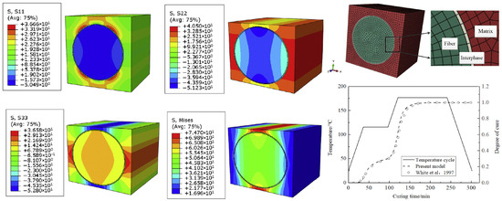
Figure 9.
Finite element analysis of residual stresses in a fibre-reinforced polymer composite during the curing process. The stress contour plots show the distributions of the normal stresses , , and , and von Mises stress in the fibre–matrix representative volume element (RVE), capturing stress gradients around the fibre and interphase region. The meshed RVE model highlights the fibre, interphase, and matrix regions. The curing cycle, including the temperature profile and degree of cure over time, is compared with the model results and data from [38].
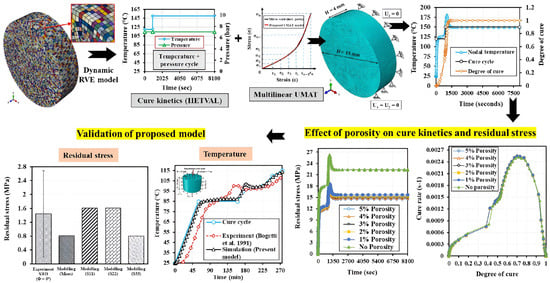
Figure 10.
Multiscale model showing the effect of porosity on cure kinetics and residual stress in composites. The model combines temperature, pressure, cure kinetics, and material behaviour. Results are validated with experiments and show that higher porosity increases residual stress and affects the cure rate [40].
Table 3.
Selected numerical contributions evaluating flow and/or thermo-chemical-induced loads for structural analysis.
5. Conclusions
This review has presented a comparative analysis of the finite element (FEM) and finite volume (FVM) methods in the context of composite manufacturing, with emphasis on their mathematical formulation and application in modelling multiscale, multiphysics phenomena. The discussion of fluid–structure interaction (FSI) further highlights the importance of coupled modelling in capturing the dynamic behaviour between fluid and solid domains during processing. By integrating theoretical insights with numerical strategies, this work underscores the potential of simulation-driven approaches to enhance process understanding, prediction, and optimization in the manufacturing of advanced composite structures. Continued development of efficient and robust computational frameworks remains essential for future advancements in this field.
Author Contributions
Conceptualisation, H.A. and M.J.; investigation, H.A.; methodology, H.A.; writing—original draft, H.A.; writing—review and editing, H.A., M.J. and C.S.; supervision; M.J., and C.S. All authors have read and agreed to the published version of the manuscript.
Funding
This research received no external funding.
Data Availability Statement
Data is contained within the article and its references.
Conflicts of Interest
The authors declare no conflicts of interest.
Appendix A. Fluid Flow, Heat Transfer, and Species Transport
During manufacturing, liquid resin—a prepolymer—exhibits fluid flow behaviour primarily dominated by convection when exposed to elevated temperatures (above room temperature). The physical processes governing this include fluid flow, heat transfer, and chemical species transport, represented mathematically by partial differential equations (PDEs) suitable for numerical treatment. These equations are discretized at nodes or control volumes depending on whether the finite element method (FEM) or finite volume method (FVM) is applied.
Appendix A.1. Flow Model
Fluid motion is described using the incompressible Navier–Stokes equations coupled with the continuity equation, which capture viscous flow dynamics as given below in Equations (A1) and (A2):
Here, denotes the average velocity field, the pressure gradient, the body force term, and represents viscous diffusion. The inertial forces are represented on the left-hand side of the momentum equation. Given that Liquid Composite Moulding (LCM) processes typically occur under slow flow conditions—characterized by a very low Reynolds number ()—viscous forces dominate and inertial terms become negligible. This simplification reduces the Navier–Stokes equations to the Stokes flow equations, which model fluid flow primarily in open regions between fibre tows— see Equations (A3) and (A4) [42,43,44,45,46]. To account for flow within porous regions (intra-tow), a source term () is introduced, leading to the Stokes–Brinkman equation. This incorporates the micro-permeability tensor , as shown in Equation (A5), which varies along directions parallel and perpendicular to fibres and can be estimated using established theoretical or analytical models [47,48,49,50,51,52,53].
When resin viscosity varies during moulding due to heat-induced curing or catalysts, chemo-rheological models such as the Castro–Macosko model [54]—Equation (A6)—are used. This model incorporates time-, temperature-, and cure-dependent viscosity changes into the governing equations. Parameters include the degree of cure , gelation point , activation energy , temperature T, gas constant R, and pre-exponential factors (, a, b).
Appendix A.2. Heat Transfer and Species Transport Models
Typically, resin infusion during mould filling can be modelled assuming constant viscosity and negligible polymerization effects, using just the continuity and momentum equations. However, when thermal effects or additives are present, the problem becomes a coupled convection–diffusion–reaction system requiring simultaneous solution of flow, energy, and species transport equations throughout impregnation and curing.
In low-velocity processes such as Resin Transfer Moulding (RTM) or Vacuum-Assisted Resin Transfer Moulding (VARTM), the Péclet number is very low, indicating local thermal equilibrium and justifying the neglect of thermal dispersion and viscous heating in the energy equation—the below Equation (A7) [55,56,57,58,59,60].
Material properties such as density , specific heat , and thermal conductivity k define the thermal response, while porosity and weight fraction w characterize the composite’s fibre and resin phases. The heat released () during curing is modelled as a source term in the energy balance, with reaction kinetics often described by an autocatalytic nth-order model (see Equation (A9)) involving pre-exponential factors (, ), reaction orders (m, n), and activation energies (, ) [61,62,63].
Dimensionless numbers such as the Graetz number (Equation (A12)) and Péclet number (Equation (A13)) play key roles in characterizing transport phenomena, determining the relative importance of conduction, convection, and dispersion [59,60]. h is the height of the mould cavity, L indicates the characteristic in-plane length of the mould, and refers to the diameter of fibres.
During the LCM process, the degree of cure is treated as a scalar field governed by the species transport Equation (A14), which accounts for transient, convective, and reactive contributions and is coupled to the energy equation through heat generation from the curing reaction.
References
- Advani, S.; Sozer, E. Liquid molding of thermoset composites. In Comprehensive Composite Materials; Elsevier: Amsterdam, The Netherlands, 2000; pp. 807–844. [Google Scholar] [CrossRef]
- Das, B.; Steinberg, S.; Weber, S.; Schaffer, S. Finite difference methods for modeling porous media flows. Transp. Porous Media 1994, 17, 171–200. [Google Scholar] [CrossRef]
- Shabro, V.; Torres-Verdín, C.; Javadpour, F.; Sepehrnoori, K. Finite-difference approximation for fluid-flow simulation and calculation of permeability in porous media. Transp. Porous Media 2012, 94, 775–793. [Google Scholar] [CrossRef]
- Belov, E.; Lomov, S.; Verpoest, I.; Peters, T.; Roose, D.; Parnas, R.; Hoes, K.; Sol, H. Modelling of permeability of textile reinforcements: Lattice Boltzmann method. Compos. Sci. Technol. 2004, 64, 1069–1080. [Google Scholar] [CrossRef]
- Eshghinejadfard, A.; Daróczy, L.; Janiga, G.; Thévenin, D. Calculation of the permeability in porous media using the lattice Boltzmann method. Int. J. Heat Fluid Flow 2016, 62, 93–103. [Google Scholar] [CrossRef]
- Liu, H.; Kang, Q.; Leonardi, C.R.; Schmieschek, S.; Narváez, A.; Jones, B.D.; Williams, J.R.; Valocchi, A.J.; Harting, J. Multiphase lattice Boltzmann simulations for porous media applications: A review. Comput. Geosci. 2016, 20, 777–805. [Google Scholar] [CrossRef]
- Sadd, M.H. 15—Numerical Finite and Boundary Element Methods. In Elasticity; Sadd, M.H., Ed.; Academic Press: Burlington, NJ, USA, 2005; pp. 413–436. [Google Scholar] [CrossRef]
- Kibrete, F.; Trzepieciński, T.; Gebremedhen, H.S.; Woldemichael, D.E. Artificial intelligence in predicting mechanical properties of composite materials. J. Compos. Sci. 2023, 7, 364. [Google Scholar] [CrossRef]
- Karuppusamy, M.; Thirumalaisamy, R.; Palanisamy, S.; Nagamalai, S.; El Sayed Massoud, E.; Ayrilmis, N. A review of machine learning applications in polymer composites: Advancements, challenges, and future prospects. J. Mater. Chem. A 2025, 13, 16290–16308. [Google Scholar] [CrossRef]
- Wu, L.; Nguyen, V.D.; Kilingar, N.G.; Noels, L. A recurrent neural network-accelerated multi-scale model for elasto-plastic heterogeneous materials subjected to random cyclic and non-proportional loading paths. Comput. Methods Appl. Mech. Eng. 2020, 369, 113234. [Google Scholar] [CrossRef]
- Yang, C.; Kim, Y.; Ryu, S.; Gu, G.X. Using convolutional neural networks to predict composite properties beyond the elastic limit. MRS Commun. 2019, 9, 609–617. [Google Scholar] [CrossRef]
- Wang, Y.; Soutis, C.; Ando, D.; Sutou, Y.; Narita, F. Application of deep neural network learning in composites design. Eur. J. Mater. 2022, 2, 117–170. [Google Scholar] [CrossRef]
- Gunzburger, M.D. Chapter 3—Navier-Stokes equations for incompressible flows: Finite-element methods. In Handbook of Computational Fluid Mechanics; Peyret, R., Ed.; Academic Press: London, UK, 1996; pp. 99–157. [Google Scholar] [CrossRef]
- Brenner, S.C.; Scott, L.R. The Mathematical Theory of Finite Element Methods, 3rd ed.; Number 15 in Texts in Applied Mathematics; Springer: New York, NY, USA, 2008. [Google Scholar]
- Donea, J.; Huerta, A. Finite Element Methods for Flow Problems, 1st ed.; Wiley: Hoboken, NJ, USA, 2003. [Google Scholar] [CrossRef]
- Elman, H.; Silvester, D.; Wathen, A. Finite Elements and Fast Iterative Solvers: With Applications in Incompressible Fluid Dynamics, 2nd ed.; Oxford University Press: Oxford, UK, 2014. [Google Scholar] [CrossRef]
- Tan, H.; Pillai, K.M. Multiscale modeling of unsaturated flow in dual-scale fiber preforms of liquid composite molding I: Isothermal flows. Compos. Part A Appl. Sci. Manuf. 2012, 43, 1–13. [Google Scholar] [CrossRef]
- Simacek, P.; Advani, S.G. A numerical model to predict fiber tow saturation during liquid composite molding. Compos. Sci. Technol. 2003, 63, 1725–1736. [Google Scholar] [CrossRef]
- Oliveira, I.; Amico, S.C.; Souza, J.; De Lima, A.G.B. Numerical analysis of the resin transfer molding process via pam-rtm software. Defect Diffus. Forum 2015, 365, 88–93. [Google Scholar] [CrossRef]
- Cheung, A.; Yu, Y.; Pochiraju, K. Three-dimensional finite element simulation of curing of polymer composites. Finite Elem. Anal. Des. 2004, 40, 895–912. [Google Scholar] [CrossRef]
- Sandberg, M.; Yuksel, O.; Baran, I.; Hattel, J.H.; Spangenberg, J. Numerical and experimental analysis of resin-flow, heat-transfer, and cure in a resin-injection pultrusion process. Compos. Part A Appl. Sci. Manuf. 2021, 143, 106231. [Google Scholar] [CrossRef]
- Perić, M. Finite-Volume Methods for Navier-Stokes Equations. In Fluids Under Pressure; Bodnár, T., Galdi, G.P., Nečasová, Š., Eds.; Springer International Publishing: Cham, Switzerland, 2020; pp. 575–638. [Google Scholar] [CrossRef]
- Versteeg, H.K.; Malalasekera, W. An Introduction to Computational Fluid Dynamics: The Finite Volume Method, 2nd ed.; Pearson Education Ltd.: Harlow, UK; New York, NY, USA, 2007. [Google Scholar]
- Patankar, S.V. Numerical Heat Transfer and Fluid Flow, 1st ed.; CRC Press: Boca Raton, FL, USA, 2018. [Google Scholar] [CrossRef]
- Ferziger, J.H.; Perić, M.; Street, R.L. Computational Methods for Fluid Dynamics; Springer International Publishing: Cham, Switzerland, 2020. [Google Scholar] [CrossRef]
- Grössing, H.; Stadlmajer, N.; Fauster, E.; Fleischmann, M.; Schledjewski, R. Flow front advancement during composite processing: Predictions from numerical filling simulation tools in comparison with real-world experiments. Polym. Compos. 2016, 37, 2782–2793. [Google Scholar] [CrossRef]
- Alotaibi, H.; Jabbari, M.; Soutis, C. A numerical analysis of resin flow in woven fabrics: Effect of local tow curvature on dual-scale permeability. Materials 2021, 14, 405. [Google Scholar] [CrossRef] [PubMed]
- Wei, B.J.; Chuang, Y.C.; Wang, K.H.; Yao, Y. Model-assisted control of flow front in resin transfer molding based on real-time estimation of permeability/porosity ratio. Polymers 2016, 8, 337. [Google Scholar] [CrossRef] [PubMed]
- Alotaibi, H.; Abeykoon, C.; Soutis, C.; Jabbari, M. A numerical thermo-chemo-flow analysis of thermoset resin impregnation in lcm processes. Polymers 2023, 15, 1572. [Google Scholar] [CrossRef] [PubMed]
- Yang, W.; Liu, W.; Jia, Y.; Chen, W. Coupled filling-curing simulation and optimized design of cure cycle in liquid composite molding. Int. J. Adv. Manuf. Technol. 2024, 132, 2489–2501. [Google Scholar] [CrossRef]
- Wittemann, F.; Maertens, R.; Bernath, A.; Hohberg, M.; Kärger, L.; Henning, F. Simulation of reinforced reactive injection molding with the finite volume method. J. Compos. Sci. 2018, 2, 5. [Google Scholar] [CrossRef]
- Shojaei, A.; Reza Ghaffarian, S.; Mohammad Hossein Karimian, S. Three-dimensional process cycle simulation of composite parts manufactured by resin transfer molding. Composite Structures 2004, 65, 381–390. [Google Scholar] [CrossRef]
- Hou, G.; Wang, J.; Layton, A. Numerical methods for fluid-structure interaction—A review. Commun. Comput. Phys. 2012, 12, 337–377. [Google Scholar] [CrossRef]
- Sigrist, J.F. Fluid-Structure Interaction: An Introduction to Finite Element Coupling; Wiley: Chichester, UK, 2015. [Google Scholar]
- Modarres-Sadeghi, Y. Introduction to Fluid-Structure Interactions; Springer International Publishing: Cham, Switzerland, 2021. [Google Scholar] [CrossRef]
- Richter, T. Fluid-structure interactions: Models, analysis and finite elements. In Lecture Notes in Computational Science and Engineering; Springer International Publishing: Cham, Switzerland, 2017; Volume 118. [Google Scholar] [CrossRef]
- Alotaibi, H.; Soutis, C.; Zhang, D.; Jabbari, M. A numerical framework of simulating flow-induced deformation during liquid composite moulding. J. Compos. Sci. 2024, 8, 401. [Google Scholar] [CrossRef]
- Yuan, Z.; Wang, Y.; Yang, G.; Tang, A.; Yang, Z.; Li, S.; Li, Y.; Song, D. Evolution of curing residual stresses in composite using multi-scale method. Compos. Part B Eng. 2018, 155, 49–61. [Google Scholar] [CrossRef]
- Gonçalves, P.T.; Arteiro, A.; Rocha, N.; Pina, L. Numerical analysis of micro-residual stresses in a carbon/epoxy polymer matrix composite during curing process. Polymers 2022, 14, 2653. [Google Scholar] [CrossRef]
- Dewangan, B.; Chakladar, N. Modelling of residual stress during curing of a polymer under autoclave conditions and experimental validation. Comput. Mater. Sci. 2024, 241, 113038. [Google Scholar] [CrossRef]
- Kim, D.H.; Kim, S.W.; Lee, I. Evaluation of curing process-induced deformation in plain woven composite structures based on cure kinetics considering various fabric parameters. Compos. Struct. 2022, 287, 115379. [Google Scholar] [CrossRef]
- Hwang, W.R.; Advani, S.G. Numerical simulations of Stokes–Brinkman equations for permeability prediction of dual scale fibrous porous media. Phys. Fluids 2010, 22, 113101. [Google Scholar] [CrossRef]
- Kuentzer, N.; Simacek, P.; Advani, S.G.; Walsh, S. Permeability characterization of dual scale fibrous porous media. Compos. Part A Appl. Sci. Manuf. 2006, 37, 2057–2068. [Google Scholar] [CrossRef]
- Parnas, R.S.; Salem, A.J.; Sadiq, T.A.; Wang, H.P.; Advani, S.G. The interaction between micro- and macro-scopic flow in RTM preforms. Compos. Struct. 1994, 27, 93–107. [Google Scholar] [CrossRef]
- Parseval, Y.D.; Pillai, K.M.; Advani, S.G. A simple model for the variation of permeability due to partial saturation in dual scale porous media. Transp. Porous Media 1997, 27, 243–264. [Google Scholar] [CrossRef]
- Gascón, L.; García, J.A.; Le Bel, F.; Ruiz, E.; Trochu, F. A two-phase flow model to simulate mold filling and saturation in Resin Transfer Molding. Int. J. Mater. Form. 2016, 9, 229–239. [Google Scholar] [CrossRef]
- Happel, J. Viscous flow relative to arrays of cylinders. AIChE J. 1959, 5, 174–177. [Google Scholar] [CrossRef]
- Sangani, A.S.; Acrivos, A. Slow flow past periodic arrays of cylinders with application to heat transfer. Int. J. Multiph. Flow 1982, 8, 193–206. [Google Scholar] [CrossRef]
- Drummond, J.E.; Tahir, M.I. Laminar viscous flow through regular arrays of parallel solid cylinders. Int. J. Multiph. Flow 1984, 10, 515–540. [Google Scholar] [CrossRef]
- Gutowski, T.G.; Cai, Z.; Bauer, S.; Boucher, D.; Kingery, J.; Wineman, S. Consolidation experiments for laminate composites. J. Compos. Mater. 1987, 21, 650–669. [Google Scholar] [CrossRef]
- Gebart, B.R. Permeability of unidirectional reinforcements for RTM. J. Compos. Mater. 1992, 26, 1100–1133. [Google Scholar] [CrossRef]
- Cai, Z.; Berdichevsky, A.L. An improved self-consistent method for estimating the permeability of a fiber assembly. Polym. Compos. 1993, 14, 314–323. [Google Scholar] [CrossRef]
- Phelan, F.R.; Wise, G. Analysis of transverse flow in aligned fibrous porous media. Compos. Part A Appl. Sci. Manuf. 1996, 27, 25–34. [Google Scholar] [CrossRef]
- Castro, J.M.; Macosko, C.W. Studies of mold filling and curing in the reaction injection molding process. AIChE J. 1982, 28, 250–260. [Google Scholar] [CrossRef]
- Bruschke, M.V.; Advani, S.G. A numerical approach to model non-isothermal viscous flow through fibrous media with free surfaces. Int. J. Numer. Methods Fluids 1994, 19, 575–603. [Google Scholar] [CrossRef]
- Abbassi, A.; Shahnazari, M.R. Numerical modeling of mold filling and curing in non-isothermal RTM process. Appl. Therm. Eng. 2004, 24, 2453–2465. [Google Scholar] [CrossRef]
- Shojaei, A.; Ghaffarian, S.R.; Karimian, S.M. Modeling and simulation approaches in the resin transfer molding process: A review. Polym. Compos. 2003, 24, 525–544. [Google Scholar] [CrossRef]
- Antonucci, V.; Giordano, M.; Nicolais, L.; Di Vita, G. A simulation of the non-isothermal resin transfer molding process. Polym. Eng. Sci. 2000, 40, 2471–2481. [Google Scholar] [CrossRef]
- Liu, B.; Advani, S.G. Operator splitting scheme for 3-D temperature solution based on 2-D flow approximation. Comput. Mech. 1995, 16, 74–82. [Google Scholar] [CrossRef]
- Dessenberger, R.B.; Tucker, C.L. Thermal dispersion in resin transfer molding. Polym. Compos. 1995, 16, 495–506. [Google Scholar] [CrossRef]
- Kamal, M.R.; Sourour, S. Kinetics and thermal characterization of thermoset cure. Polym. Eng. Sci. 1973, 13, 59–64. [Google Scholar] [CrossRef]
- Sourour, S.; Kamal, M.R. Differential scanning calorimetry of epoxy cure: Isothermal cure kinetics. Thermochim. Acta 1976, 14, 41–59. [Google Scholar] [CrossRef]
- Kamal, M.R. Thermoset characterization for moldability analysis. Polym. Eng. Sci. 1974, 14, 231–239. [Google Scholar] [CrossRef]
Disclaimer/Publisher’s Note: The statements, opinions and data contained in all publications are solely those of the individual author(s) and contributor(s) and not of MDPI and/or the editor(s). MDPI and/or the editor(s) disclaim responsibility for any injury to people or property resulting from any ideas, methods, instructions or products referred to in the content. |
© 2025 by the authors. Licensee MDPI, Basel, Switzerland. This article is an open access article distributed under the terms and conditions of the Creative Commons Attribution (CC BY) license (https://creativecommons.org/licenses/by/4.0/).