Managing Surcharge Risk in Strategic Fleet Deployment: A Partial Relaxed MIP Model Framework with a Case Study on China-Built Ships

Abstract

Container liner shipping companies operate within a complex environment where they must balance profitability and service reliability. Meanwhile, evolving regulatory policies, such as surcharges imposed on ships of a particular origin or type on specific trade lanes, introduce new operational challenges. This study addresses the heterogeneous ship routing and demand acceptance problem, aiming to maximize two conflicting objectives: weekly profit and total transport volume. We formulate the problem as a bi-objective mixed-integer programming model and prove that the ship chartering constraint matrix is totally unimodular, enabling the reformulation of the model into a partially relaxed MIP that preserves optimality while improving computational efficiency. We further analyze key mathematical properties showing that the Pareto frontier consists of a finite union of continuous, piecewise linear segments but is generally non-convex with discontinuities. A case study based on a realistic liner shipping network confirms the model’s effectiveness in capturing the trade-off between profit and transport volume. Sensitivity analyses show that increasing freight rates enables higher profits without large losses in volume. Notably, this paper provides a practical risk management framework for shipping companies to enhance their adaptability under shifting regulatory landscapes.

1. Introduction

Container liner shipping is a cornerstone of global trade, enabling the efficient transport of goods across continents and supporting much of the world’s economic activity [1]. In 2025, however, the transpacific shipping market and the broader containerized ocean transport system are experiencing significant disruptions due to new U.S. Section 301 actions targeting ships built in China or operated by Chinese companies [2,3,4]. These measures impose phased port surcharges, effective after a 180-day grace period starting 17 April 2025, with fees for Chinese ship owners/operators beginning at $50 per net ton per U.S. voyage and escalating to $140 per net ton by 17 April 2028 [5]. For China-built ships operated by non-China entities, fees start at $18 per net ton (or $120 per container unloaded) and rise to $33 per net ton (or $250 per container) by the same date, applied up to five times annually per ship [5]. Additionally, the policy mandates that a growing share of U.S. exports, such as liquefied natural gas (LNG), be carried on U.S.-operated ships, starting at 1% in 2028 and increasing to 15% by 2047 [2]. These measures have already caused significant disruptions across key sectors. In the coal sector, ship owners are refusing U.S. coal shipment contracts due to the cost increases, halting $130 billion in exports within 60 days, as the fees have raised delivered coal costs by up to 35% [6]. Agricultural exporters of corn, soybeans, and wheat are struggling to secure ocean freight since May 2025, incurring additional transportation costs of $372 million to $930 million annually [6]. Energy exports, including LNG and oil, are being curtailed due to the absence of non-China-built ships, significantly impacting shipments [6]. Operationally, carriers are suspending routes to smaller ports like Oakland in favor of larger hubs like Los Angeles, causing congestion and equipment misallocation [7]. Industry estimates indicate the fees are adding $600–$800 per container, costing the shipping sector $20 billion annually and increasing consumer prices [7]. These disruptions highlight the urgency and scale of the policy shock, underscoring the need for stakeholders to adapt swiftly to mitigate economic fallout.

Liner operators, already navigating a highly competitive and volatile market [8], must now grapple with these profound regulatory changes in addition to existing challenges such as fluctuating demand, rising operating costs, and increasing ship heterogeneity stemming from fleet expansion and alliance strategies [8,9]. This significantly complicates key decisions in operational management [9], including ship routing, fleet deployment, and transport demand acceptance, which must be carefully balanced to maintain competitiveness [10]. The introduction of such significant port surcharges based on ship origin and ownership fundamentally alters ship routing and deployment decisions. Prior studies on ship routing and scheduling emphasize that changes in cost structures, such as the imposition of new regional fees, directly affect optimal fleet routing, port call patterns, and service frequency [4,11,12]. When operational costs increase on specific routes or port calls, liner operators have strong incentives to adjust their deployment, potentially discontinuing routes that include high-fee ports to minimize surcharge exposure [4]. Empirical research and optimization models show that fleet deployment decisions are highly sensitive to regulatory and cost-driven shocks [13], with dynamic re-routing occurring not only in response to fuel price shifts and emission control area (ECA) regulations, but also as shippers and carriers seek least-cost pathways under new port or trade restrictions [14]. Consequently, shipping lines have begun reviewing fleet composition, revisiting newbuilding strategies, and considering detaching beneficial ownership links to avoid U.S. surcharges, potentially transferring China-built ships to non-U.S. trades or substituting other nations’ builds into U.S. lanes [2,4].

Against this backdrop of specific and evolving regulatory challenges, including changing cost structures, environmental rules, and geopolitical pressures, existing research has extensively studied a wide range of operational decisions in liner shipping, particularly in areas such as multi-route scheduling, fleet deployment under cost variability, ship speed optimization, and port time windows. Numerous studies develop optimization models for ship routing and scheduling, addressing both industrial and tramp segments as well as liner shipping, and often tackle multi-ship, multi-route scenarios, variable ship speeds, and constraints arising from port schedules and ship heterogeneity [11,12,15,16,17]. These frequently employ mathematical programming techniques like mixed-integer linear programming (MILP), mixed-integer nonlinear programming (MINLP), and advanced heuristic methods to handle large-scale, realistic instances [12]. Given the inherent trade-offs in liner shipping operations between economic performance, service quality, energy consumption, and environmental regulations, multi-objective optimization frameworks have gained prominence for addressing these complex decisions [18]. These frameworks aim to identify effective operational strategies by considering divergent objectives like cost minimization, profit maximization, service coverage, and on-time delivery, with much research dedicated to finding robust solutions in these multifaceted decision environments [18,19,20]. Separately, the critical role of demand acceptance in revenue management is also well established, with numerous studies addressing its optimization, particularly for scenarios involving transit-time-sensitive demand [21]. These studies highlight effective strategies for maximizing revenue based on demand characteristics. While both multi-objective optimization and demand acceptance are individually well explored, their integration within comprehensive models for optimizing ship routing, fleet deployment, and service design, particularly for models that must also account for dynamic slot allocation alongside periodic demand structures or heterogeneous fleet operations, represents an area with ongoing research opportunities [22]. In tackling such comprehensive models, they must incorporate complexities like ship heterogeneity, multi-objective trade-offs, and general regulatory constraints [12,17].

In addition, the latest U.S. measures underscore a more profound research gap: while operational decision making under general regulatory and cost constraints has been widely examined, most existing research on fleet deployment and ship routing does not fully account for the specific impacts of regulatory measures like Section 301 surcharges, which are based on a ship’s country of build or ownership [23]. Most prior studies on ship routing and fleet deployment assume homogeneous fleets or do not explicitly model the bi-objective trade-offs, indicating a clear lack of integrated models that simultaneously optimize heterogeneous ship routing in the context of specific and impactful regulatory shocks such as the Section 301 surcharges. Even when general regulatory constraints are considered, analyses rarely examine the specific operational impacts of surcharges differentiated by ship build country on route selection, ship assignment with particular attention to China-built ships compared to others, and transport demand acceptance strategies within a unified bi-objective optimization framework. Such a framework should incorporate both operational heterogeneity and policy-driven risks. There is a clear need for new models to investigate the consequences of these policies, especially regarding global fleet renewal, cross-border cargo flows, and the resilience and adaptability of international shipping networks amid shifting regulatory landscapes.

To address these gaps comprehensively, this study formulates a heterogeneous ship routing and demand acceptance (HSR-DA) problem under the influence of U.S. regulatory surcharges on China-built ships. The HSR-DA problem jointly optimizes route operation, heterogeneous ship assignments, transport demand acceptance, and chartering decisions with the dual objectives of maximizing weekly profit and total transport volume. A bi-objective mixed-integer programming (MIP) model is developed to support integrated decision making, incorporating practical constraints such as ship requirements, fleet availability considering chartering, accepted transport volume, and transport capacity limits. To enhance computational efficiency, this study further introduces a partially relaxed mixed-integer programming (PRMIP) model by leveraging the TU properties of the chartering constraint matrices, which significantly reduces computational complexity without compromising optimality. Overall, the proposed bi-objective MIP model provides a practical and implementable optimization framework for shipping companies seeking to adapt their operations optimally in response to challenging regulatory landscapes.

In particular, the multifaceted contributions of this paper are outlined as follows:

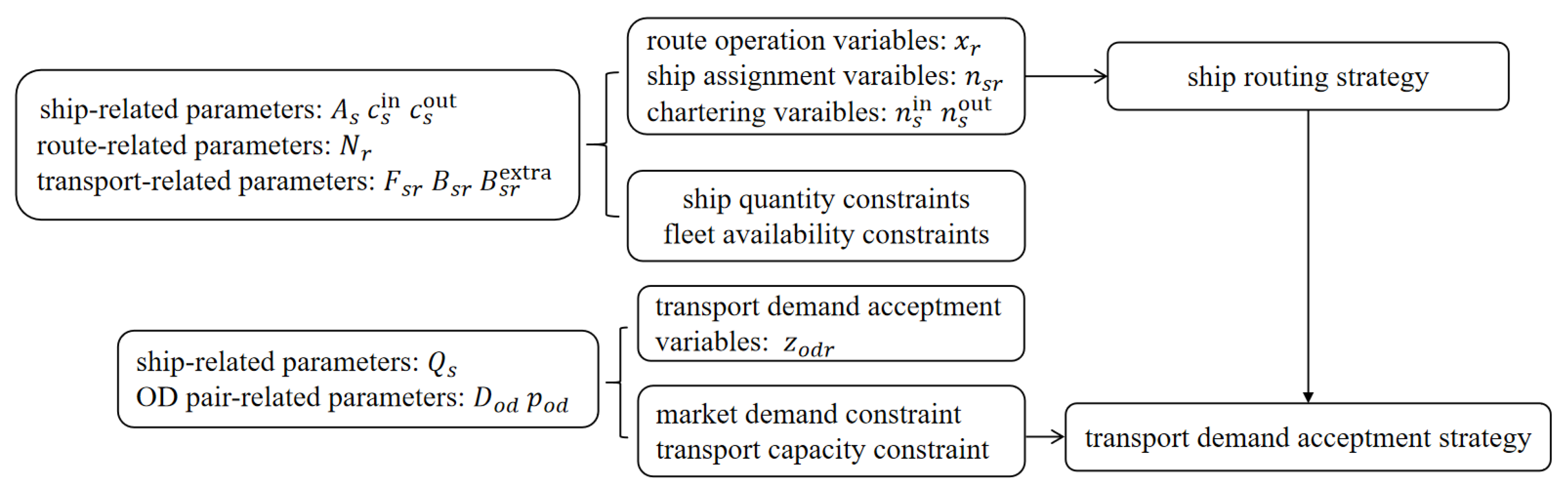
• We establish a bi-objective MIP model for jointly optimizing the heterogeneous ship routing and transport demand acceptance, subject to ship requirement constraints, fleet availability and demand acceptance limits. This formulation enables shipping companies to effectively evaluate and strategically balance the often competing objectives of maximizing weekly profit and maximizing total transport volume, thereby facilitating more informed decision making in their operational planning and resource allocation under the new regulatory pressures.
• We prove the necessity of maintaining integrality for route operation variables and ship assignment variables and develop a computationally efficient PRMIP model by leveraging the totally unimodular (TU) property of the chartering constraint matrices, allowing for continuous relaxation of the ship chartering variables without compromising optimality. The model is validated through a real-world case study, which shows that the PRMIP model achieves identical optimal solutions to the MIP model with significantly reduced computational time.
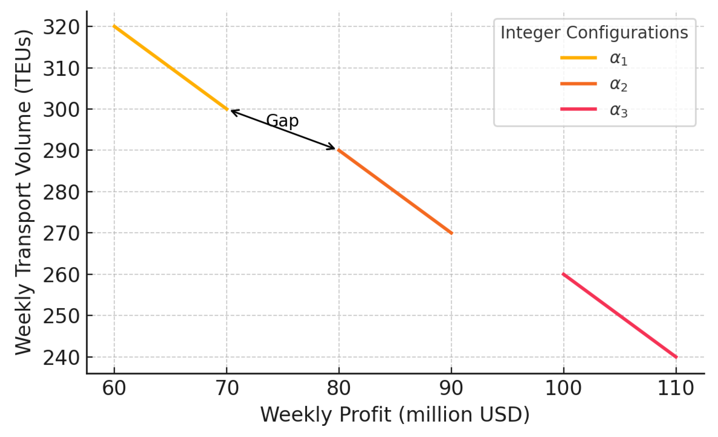
• We analyze the structural properties of the Pareto frontier for the bi-objective MIP model and find that it consists of a finite union of continuous, piecewise linear segments. We also show that the global frontier is generally non-convex and can exhibit discontinuities due to the discrete nature of ship assignment and route operation decisions. This structural insight provides a precise characterization of the optimal trade-offs between profit maximization and transport volume, illuminating the set of efficient solutions.
• Sensitivity analyses demonstrate that as freight rates increase, the Pareto frontier shifts to offer simultaneously improved profitability and transport volume potential. This shift shows diminished marginal trade-offs between the two objectives, enhancing operational flexibility.
• A case study based on a global liner network, considering the impact of U.S. surcharges, yields three major managerial insights: (i) optimal fleet deployment under the surcharges consistently involves avoiding the assignment of China-built ships to routes serving U.S. ports to minimize regulatory cost impacts; (ii) strategic selection of an operating point on the profit-volume Pareto frontier is crucial, as an extreme focus on one objective leads to disproportionate sacrifices in the other, underscoring the practical value of balanced operational strategies; and (iii) prioritizing profitability naturally drives route network rationalization and selective acceptance of higher-value cargo, which in turn reduces overall operational costs and optimizes fleet utilization.

The remainder of this paper is structured as follows. Section 2 provides an overview of the relevant literature on liner shipping optimization, fleet deployment, demand acceptance, and the impact of regulatory policies. Section 3 formulates the research problem as a bi-objective MIP model and presents its theoretical properties. Section 4 details the augmented $ϵ$-constraint method adopted to solve the bi-objective optimization model. Section 5 reports the numerical results and sensitivity experiments. Finally, Section 6 concludes the paper and outlines directions for future research.

2. Literature Review

To comprehensively understand the methodologies for ship routing, fleet deployment, and transport demand acceptance under regulatory pressures, this review examines the literature focusing on optimization models and algorithms for HSR-DA within liner shipping operational frameworks.

2.1. Ship Routing, Fleet Deployment, and Demand Acceptance

Several studies investigate the optimization of ship routing and fleet deployment under complex operational constraints. Christiansen et al. provide a comprehensive overview, addressing network design, ship routing, and speed optimization, emphasizing the necessity of integrated decision making to enhance operational efficiency [1]. Tran and Haasis review network optimization, highlighting that routing decisions must carefully account for port capacity constraints, vessel types, and market demand characteristics, typically employing mathematical programming to minimize total operational costs [24].

To minimize costs or maximize profits, Gu et al. develop a model for fleet deployment and speed optimization, explicitly considering fuel consumption heterogeneity, through integrated decisions on node selection, ship assignment, and speed setting [25]. Jiang et al. construct a MILP model to optimize route and schedule design within port time window constraints [26]. Zheng et al. propose a MILP model combined with global optimization algorithms to handle heterogeneous fleets and reduce total operational costs [18]. Multi-objective approaches are also proposed in response to environmental and regulatory pressures. Pasha et al. introduce a tactical-level joint optimization model for heterogeneous fleets, balancing CO₂ emissions reduction and profit maximization [27]. Zhao et al. incorporate low-carbon operations and fuel bunkering into a cost-minimization model for greener shipping [28]. Tran and Haasis survey various multi-objective strategies addressing multiple performance indicators including customer satisfaction and carbon emissions [24]. To solve large-scale container liner shipping optimization problems, researchers formulate MILP or MINLP models and employ exact algorithms, heuristics, and matheuristics [25,27,28,29].

Demand acceptance optimization is also receiving increasing attention. Cheaitou et al. model time-sensitive demand using integer nonlinear programming and heuristics to maximize profit [30]. Pasha et al. propose a holistic MILP model that integrates demand elasticity with fleet deployment and speed optimization [10]. Xia et al. consider joint planning of cargo allocation, speed, and fleet deployment to minimize fuel and operational costs [31]. Lai et al. adopt a two-stage robust optimization framework under demand uncertainty [32], while Zhao et al. summarize multi-objective planning approaches for demand acceptance, focusing on tonnage limits and route capacity [33].

2.2. Impact of Regulatory Policies and External Disruptions

Regulatory policies profoundly influence container liner shipping by imposing constraints that reshape routing, fleet deployment, and demand acceptance strategies, compelling operators to balance compliance with cost efficiency. Environmental regulations, such as sulfur emission caps and carbon reduction targets, promote sustainable practices. Psaraftis and Kontovas demonstrate through speed optimization models how minimizing fuel costs and emissions via measures like low sulfur fuel or speed reductions can increase operational costs by up to 20% [34]. Pasha et al. optimize tactical planning using a model that incorporates carbon taxes and varied ship efficiencies, achieving considerable emission reductions alongside cost minimization [27]. Zhao et al. propose a model for green liner shipping that balances costs and emissions through fleet deployment and fuel bunkering, resulting in significant emission reductions [28]. Trade policies, such as proposed U.S. surcharges on certain foreign built ships involving substantial fees per port call, necessitate rerouting or fleet reconfiguration [3]. Bertho et al. use regression-based econometric analysis to show that foreign investment restrictions raise shipping costs by 24–50% and reduce trade flows, necessitating adaptive routing models [35]. Notteboom et al. and Fan et al. apply descriptive statistics and network modeling to highlight how U.S.–China trade tensions increase operating costs by 5–10% and transit times by up to 12% on Asia–North America routes [36]. Safety regulations, for instance the International Ship and Port Facility Security Code, extend port turnaround times by 10–20%, indirectly increasing costs, as Bichou’s qualitative analysis indicates [37]. These studies underscore the need for optimization models that incorporate specific regulatory constraints.

External disruptions, including pandemics, geopolitical events, and natural disasters, exacerbate operational challenges in liner shipping, requiring resilient strategies to mitigate delays and costs. The COVID-19 pandemic, as Jin et al. show through AIS-driven data analysis, reduced China’s port network connectivity by 15% due to congestion, while Notteboom’s descriptive analysis reports a 20% rise in schedule disruptions, prompting network reconfiguration [38]. Ksciuk et al. propose a simulation-based optimization model, integrating simulation and optimization techniques to manage pandemic induced congestion, reducing delays and costs by up to 25% through optimized ship assignments [39]. Zhu et al. develop exact branch and bound and metaheuristic algorithms to optimize vessel deployment and routing under congestion, achieving 8–12% cost savings [40]. The 2021 Suez Canal blockage, which caused substantial daily trade losses according to Verschuur et al.’s economic modeling, necessitated rerouting via the Cape of Good Hope, increasing transit times by 10–14 days [41]. Elmi et al. advocate port skipping, which their review shows can reduce delays by up to 20% [42]. Natural disasters, addressed by Zheng et al.’s distributed predictive control model, require rapid rerouting to minimize response times [43].

2.3. Recent Trends in Multi-Objective Optimization

Recent advancements in multi-objective optimization provide methodologies that can inspire solutions for ship routing, fleet deployment, and demand acceptance in liner shipping. For instance, skip-stop strategies in urban rail transit optimize total travel time and equity in service distribution. Han et al. [44] formulate a multi-objective mixed integer nonlinear programming model to minimize both inequity and total travel time through train stop planning and scheduling, with a case study on Seoul’s urban railways. Rajabighamchi et al. [45] propose a robust multi-objective model for skip-stop scheduling, minimizing travel and waiting times while ensuring equitable service through robust scheduling under demand uncertainty. Shang et al. [46] address passenger crowding risks and revenue losses in oversaturated networks, offering insights for port call sequence optimization in liner shipping under congestion or regulatory constraints. Similarly, accessible routing strategies provide inspiration for customized routing; Lee et al. [47] develop an accessible taxi routing model based on the travel behavior of people with disabilities, using a Gaussian mixture model to optimize routes, which can guide prioritization of ports with specialized cargo needs. Additionally, Lee and Kim [48] develop a multi-objective model for submerged floating tunnel routing, balancing structural safety and travel time using Non-dominated Sorting Genetic Algorithm II (NSGA-II), achieving 9.9% to 10.5% time savings on the Mokpo–Jeju route. These techniques can inform ship routing under complex constraints like safety regulations or emission control areas.

Recent progress in liner shipping has focused on integrating multi-objective optimization with heterogeneous fleet assignment under regulatory constraints. Pasha et al. [27] propose a multi-objective MILP model for tactical-level planning in liner shipping, optimizing ship deployment and routing for heterogeneous fleets while balancing costs and CO₂ emissions under carbon tax regulations, achieving up to 15% cost savings and 20% emission reductions on a transatlantic route. Wang et al. [9] investigate co-management of heterogeneous ship fleets in liner alliances, optimizing profit-sharing, fleet utilization, and service reliability under emission caps, improving profit by 10% and reducing delays by 12% on an Asia–Europe route. Wen et al. [49] develop a multi-objective MILP model for ship scheduling, addressing port congestion and environmental regulations using queuing theory, optimizing costs, emissions, and service unreliability with improvements of 4%, 6%, and 44% over NSGA-II, applied to Maersk’s Trans-Pacific route with nine ports and five ships of 10,000 TEU. These studies highlight the potential of multi-objective MILP frameworks to balance economic, environmental, and operational objectives in liner shipping under stringent regulatory environments.

2.4. Research Gap

Despite the significant advancements in optimization models for ship routing, fleet deployment, and demand acceptance, several key gaps remain in the existing literature:

• The lack of comprehensive frameworks for coordinating ship fleet management and surging regulatory policies: While some studies have explored fleet deployment in the context of heterogeneous fleets, few models address the origin-based cost differences arising from regulatory policies, such as surcharges on certain foreign-built ships. Regulatory impacts, such as the penalties imposed on China-built ships, are often overlooked in operational models despite their significant effects on route viability and fleet deployment decisions. Christiansen et al. [1], Gu et al. [25], and Jiang et al. [26] investigate fleet deployment, but they do not consider regulatory policies like U.S. surcharges on China-built ships that directly influence fleet deployment strategies and routing decisions. Pasha et al. [27], Zhao et al. [28], and Bertho et al. [35] explore regulatory constraints like carbon taxes or fuel efficiency but do not explicitly incorporate surcharges based on ship origin or other regulatory policies into fleet deployment and routing frameworks. In contrast, our work integrates these origin-based cost differences into the optimization framework, providing a more realistic model for ship routing and fleet deployment under such regulatory pressures.
• The limited availability of integrated optimization models that jointly consider routing, fleet assignment, and demand acceptance decisions: A recurring issue in the literature is the treatment of routing, fleet assignment, and demand acceptance as separate or loosely coupled problems. This approach limits the ability to model the intricate trade-offs between short-term cost efficiency and long-term network viability, especially in markets affected by volatile demand and regulatory shocks. Song et al. [18], Jiang et al. [26], and Zhao et al. [28] develop MILP models for routing and scheduling under specific constraints but often treat fleet deployment and demand acceptance separately, missing the dynamic interactions between these components. Tran and Haasis [24] review network optimization but fail to provide a unified framework that integrates fleet deployment, routing, and demand acceptance within a single optimization model. Wang et al. [9], Pasha et al. [10], and Cheaitou et al. [30] also examine these components separately, limiting the scope of their models. Our model addresses this gap by unifying routing, fleet assignment, and demand acceptance within a single framework, enabling the consideration of trade-offs between cost, fleet utilization, regulatory constraints, and demand acceptance in an integrated manner.
• The challenge of balancing profitability and service scale under regulatory constraints: A key challenge in liner shipping optimization is the trade-off between maximizing profitability and meeting service volume targets, particularly in light of regulatory changes such as surcharges on foreign-built ships. While multi-objective optimization has been increasingly employed in shipping optimization, few models effectively address the balance between cost efficiency and service scale, especially in the context of specific regulatory pressures. Pasha et al. [27], Zhao et al. [28], and Wang et al. [9] propose multi-objective models for fleet deployment and route optimization but fail to fully address the conflict between profitability and service volume. Their models typically consider cost minimization and emission reduction without taking into account the penalties and increased costs imposed by regulatory policies. Cheaitou et al. [30], Pasha et al. [10], and Lai et al. [32] also address demand acceptance and fleet deployment but do not fully integrate the operational impact of regulatory changes on the profitability–service scale balance. Wen et al. [49] optimize ship scheduling under port congestion and environmental regulations, but their work focuses more on service reliability and emission reduction, not on explicitly balancing profitability with service volume. Our research bridges this gap by explicitly modeling the bi-objective conflict between profitability and service scale in the context of regulatory surcharges, which significantly affect route-specific costs and margins. By incorporating regulatory costs into our multi-objective optimization model, we allow liner shipping companies to make more informed decisions on how to balance profitability and service commitments.

To bridge these gaps, we propose a bi-objective MIP model designed for the HSR-DA problem, which integrates route operation, ship assignment, and transport demand acceptance. This MIP model uniquely incorporates real-world cost structures, especially surcharges such as those imposed on China-built ships. These surcharges are embedded in the objective function and play a critical role in shaping routing and deployment decisions across a heterogeneous fleet. The model formulation incorporates several practical constraints, including ship assignment limitations, fleet availability, demand-related transport volume constraints, and transport capacity requirements. This model provides a comprehensive decision-support tool for operational planning under real-world regulatory and market conditions. In particular, it provides guidance for ship routing and demand acceptance decisions under the influence of recent policy proposals to impose substantial surcharges on China-built ships calling at U.S. ports.

3. Problem Formulation

In this section, we first introduce the problem background and describe the challenges in route deployment, ship assignment, and transport demand acceptance in Section 3.1. Following that, we formulate the problem using a bi-objective MIP model in Section 3.2. Finally, Section 3.3 provides a detailed description of model analysis.

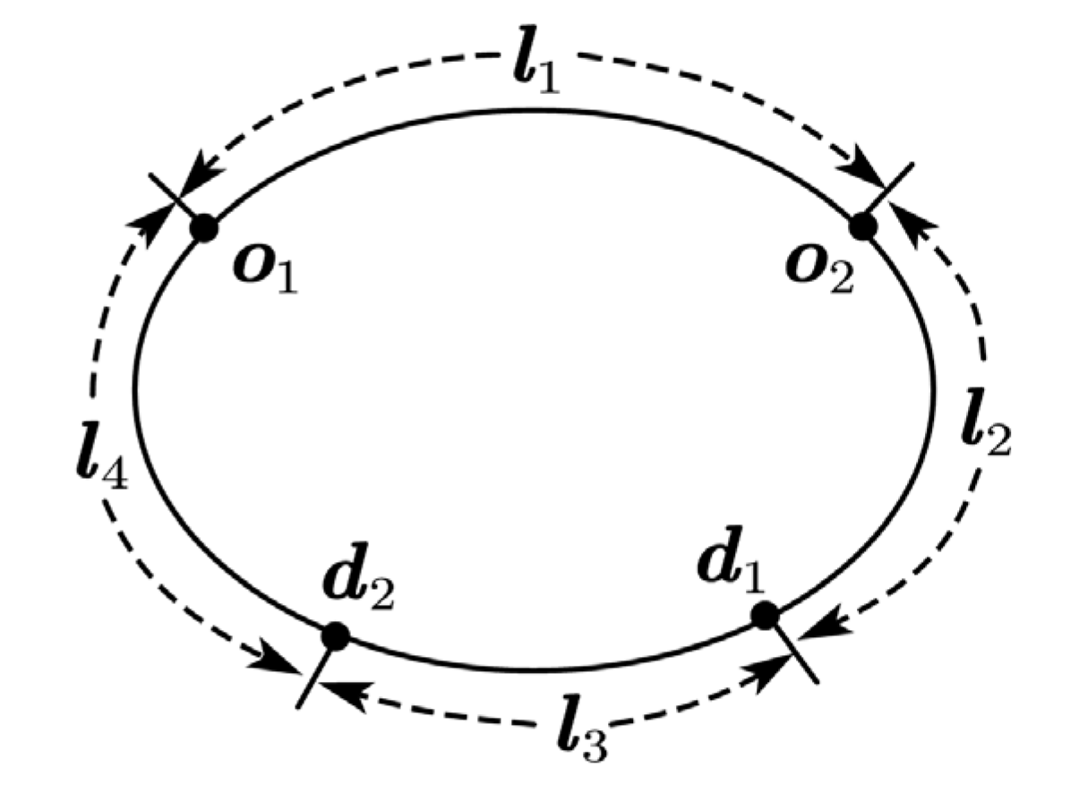
3.1. Problem Description

Container liner operators are under constant pressure to balance network coverage, asset utilization, and profitability. They must decide which cyclic routes to operate, how to deploy heterogeneous ships, and how much freight demand to accept, all while facing volatile fuel prices, charter rates, and regulatory surcharges. Recent policy proposals to levy additional port fees on China-built ships calling at U.S. ports have further complicated fleet planning. These surcharges specifically apply only to China-built ships above a certain capacity threshold, while ships constructed in other countries or smaller China-built ships are exempt [50]. As a result, carriers with mixed fleets must now carefully account for route-dependent surcharges in their cost structure. Against this backdrop, a strategic yet tractable planning framework is indispensable for maximizing profit without jeopardizing service reliability.

For the shipping company, three interdependent planning tasks are of primary importance: selecting a subset of candidate routes to operate, assigning a suitable mix of ship types to each operated route to meet the required ship count, and determining how much of the origin–destination (OD) demand to accept and how to allocate the accepted demand across the selected network. If route deployment and fleet composition are poorly matched to demand geography, high-yield OD pairs may be rejected, deployed ships may be underutilized, or routes may involve China-built ships incurring avoidable penalties at U.S. ports. In light of these considerations, it is crucial to precisely choose operating routes based on transport demand and associated costs, including fuel cost, berthing cost, and route-specific surcharges for certain ship types, and to allocate the fleet accordingly. Making informed decisions on ship deployment and chartering actions, including when to charter in and charter out ships, is vital to maintaining the cost-effectiveness and competitiveness of the operator’s network.

Consider the route–ship–demand allocation problem in a liner-shipping network that provides stable containerized services over a set of predefined cyclic routes. The set of all candidate routes is denoted by $R$ (indexed by $r$). Each route represents a predefined closed-loop trajectory involving a sequence of ports and is a candidate for service deployment with a fixed weekly schedule. The set of OD pairs is denoted by $W$, where each element $(o,d)$ indicates an origin port $o$ and a destination port $d$. For each OD pair, the subset of feasible routes that connect the two ports is denoted by $R_{od}\subseteq R$. The set of all legs between consecutive ports of call on route $r$ is denoted by $L_r$ (indexed by $l_r$). For each leg $l_r$, we denote the set of OD pairs routing passes through the leg by $W_{l_r}$ $\subseteq W$. The set of available ship types is denoted by $S$, where ships built in China are represented by the subset $\widehat{S}\subseteq S$. The available fleet includes both ships owned by the shipping company and charterable ships.

To ensure a weekly departure frequency on any operated route, a sufficient number of ships must be deployed to maintain the required frequency, given the time needed to complete a full loop. We assume that all ships sail at a uniform speed when deployed on the same route, and the total number of ships required on route $r$, denoted by $N_r$, is numerically equal to the round-trip time (in weeks) for route $r$, as one ship must depart each week while another completes the full loop.

The weekly transport demand for each OD pair is denoted by $D_{od}$, and the corresponding revenue earned per TEU transported is denoted by $p_{od}$. The total volume of accepted demand for each OD pair cannot exceed $D_{od}$, and the shipping company is allowed to reject part of the demand if full acceptance leads to unprofitable operations. Each ship type $s$ has a capacity of $Q_s$ twenty-foot equivalent units (TEUs). The transportation cost of one ship of type $s$ completing a full round trip on route $r$ includes fuel costs ($F_{sr}$), berthing costs ($B_{sr}$), and any extra penalties specifically incurred by China-built ships when deployed on routes calling at U.S. ports ($B_{sr}^{\mathrm{e}\mathrm{x}\mathrm{t}\mathrm{r}\mathrm{a}}$). The company’s owned fleet includes $A_s$ ships of type $s$. To reduce operating costs, such as avoiding penalty fees associated with deploying China-built ships on routes that call at U.S. ports, the company may choose to charter in additional ships of alternative types and charter out idle ships that are not required. The weekly cost of chartering in a ship of type $s$ is given by $c_s^{\mathrm{i}\mathrm{n}}$, and the revenue obtained from chartering out an idle ship of type $s$ is denoted by $c_s^{\mathrm{o}\mathrm{u}\mathrm{t}}$.

A route represents a complete, cyclical sequence of port calls that a ship follows. A leg is the segment of a route connecting two adjacent ports. An OD pair represents a specific transport demand from a port of origin to a port of destination, both of which lie on the same route. The path for fulfilling an OD pair’s demand consists of one or more sequential legs along the route. To visually illustrate these relationships, Figure 1 presents an illustrative diagram.

Figure 1 shows an example circle route $r$ that consists of four ports. The segments connecting adjacent ports form the four legs of the route: $l_1$, $l_2$, $l_3$, and $l_4$. The figure also illustrates two distinct OD pairs. The first is a transport demand from origin port $o_1$ to destination port $d_1$, with its path covering legs $l_1$ and $l_2$. The second is a transport demand from origin port $o_2$ to destination port $d_2$, which is fulfilled by traversing legs $l_2$ and $l_3$. This structure highlights how multiple OD demands can share capacity on common legs within a single shipping route.

The objective of this study is formulated as a bi-objective optimization that simultaneously maximizes the weekly profit and maximizes the total weekly transport volume across all OD pairs. The weekly profit consists of the total revenue from accepted transport demand, minus the total transportation costs of deployed ships, minus the cost of chartering in ships, plus the revenue generated from chartering out idle ships. To this end, we need to decide which candidate routes to operate. This decision is represented by the binary variable $x_r$, which equals 1 if route $r$ is operated, and 0 otherwise. We also determine the fleet composition on each operated route by assigning specific ship types. This is described by the integer decision variable $n_{sr}$, which indicates the number of ships of type $s$ assigned to route $r$. In addition, we consider whether ships are rented in or chartered out. The integer decision variable $n_s^{\mathrm{i}\mathrm{n}}$ denotes the number of ships of type $s$ chartered in during the planning horizon, while $n_s^{\mathrm{o}\mathrm{u}\mathrm{t}}$ represents the number of ships of type $s$ chartered out. For each OD pair $(o,d)$ and each route $r\in R_{od}$, the transport volume is determined by the continuous decision variable $z_{odr}$, which specifies the amount of accepted demand (TEUs/week) allocated to route $r$.

3.2. Model Formulation

In this subsection, we present a bi-objective MIP model based on the problem setting described above. The model captures the integrated planning decisions required for route selection, ship assignment, and demand acceptance in a container liner shipping network. It focuses on strategic decisions for which routes to operate, the type and quantity of ships assigned to each operated route, the amount of weekly transport demand for each OD pair to accept, the allocation of accepted demand across the operated routes, and the number of ships to charter in and charter out. The objective is to maximize the weekly total profit and the total weekly transport volume across all OD pairs while adhering to practical constraints such as ship assignment limitations, fleet availability, demand-related transport volume constraints, and transport capacity requirements.

Table 1. Notations used in the model formulation.

Route and OD Pair-Related Parameters
$R$	The set of all candidate routes, $r\in R$
$L_r$	The set of all legs between consecutive ports of call on route $r$, $l_r\in L_r$
$W$	The set of OD pairs, $(o,d)\in W$
$R_{od}$	The subset of feasible routes connecting $(o,d)$, $R_{od}\subseteq R$
$W_{l_r}$	The set of OD pairs that are routed via leg $l_r$, $W_{l_r}\subseteq W$
$N_r$	The total number of ships required to operate route $r$
$D_{od}$	The weekly transport demand for $(o,d)$
$p_{od}$	The revenue earned per TEU transported for $(o,d)$
Ship-Related Parameters
$S$	The set of all ship types, $s\in S$
$\widehat{S}$	The set of China-built ship types, $\widehat{S}\subseteq S$
$Q_s$	The transport capacity of a ship of type $s$
$A_s$	The number of ships of type $s$ owned by the shipping company
$c_s^{\mathrm{i}\mathrm{n}}$	The weekly cost of chartering in a ship of type $s$
$c_s^{\mathrm{o}\mathrm{u}\mathrm{t}}$	The weekly revenue from chartering out a ship of type $s$
Transport-Related Parameters
$F_{sr}$	The fuel cost of one ship of type $s$ completing one full trip on route $r$
$B_{sr}$	The berthing cost for a ship of type $s$ for a full round trip on route $r$
$B_{sr}^{\mathrm{e}\mathrm{x}\mathrm{t}\mathrm{r}\mathrm{a}}$	The extra penalty cost for a ship of type $s$ for a full round trip on route $r$
Decision Variables
$x_r$	Binary variable, which equals 1 if the candidate route $r$ is operated, and 0 otherwise
$n_{sr}$	Integer variable, indicating the number of ships of type $s$ assigned to route $r$
$n_s^{\mathrm{i}\mathrm{n}}$	Integer variable, indicating the number of ships of type $s$ chartered in
$n_s^{\mathrm{o}\mathrm{u}\mathrm{t}}$	Integer variable, indicating the number of ships of type $s$ chartered out
$z_{odr}$	Continuous variable, indicating the number of accepted TEUs per week for $(o,d)$ on route $r$

summarizes the notations used in the model.

The MIP model, formulated as Model (1), is developed to optimize route selection, ship assignment, weekly transport allocation, and chartering decisions, and can be written as follows:

max	${\displaystyle \sum _{\left(o,d\right)\in W}}{\displaystyle \sum _{r\in R_{od}}}{p}_{od}\cdot z_{odr}-{\displaystyle \sum _{r\in R}}{\displaystyle \sum _{s\in S}}{\displaystyle \frac{n_{sr}}{N_r}}\left(F_{sr}+B_{sr}\right)-{\displaystyle \sum _{r\in R}}{\displaystyle \sum _{s\in \widehat{S}}}{\displaystyle \frac{n_{sr}}{N_r}}{B}_{sr}^{\mathrm{e}\mathrm{x}\mathrm{t}\mathrm{r}\mathrm{a}}-{\displaystyle \sum _{s\in S}}{c}_s^{\mathrm{i}\mathrm{n}}\cdot n_s^{\mathrm{i}\mathrm{n}}+{\displaystyle \sum _{s\in S}}{c}_s^{\mathrm{o}\mathrm{u}\mathrm{t}}\cdot n_s^{\mathrm{o}\mathrm{u}\mathrm{t}}$		(1-1)
max	${\displaystyle \sum _{\left(o,d\right)\in W}}{\displaystyle \sum _{r\in R_{od}}}{z}_{odr}$		(1-2)
s.t.	${\displaystyle \sum _{s\in S}}{n}_{sr}=N_r\cdot x_r$	$\forall r\in R$	(1-3)
	${\displaystyle \sum _{r\in R}}{n}_{sr}\le A_s+n_s^{\mathrm{i}\mathrm{n}}-n_s^{\mathrm{o}\mathrm{u}\mathrm{t}}$	$\forall s\in S$	(1-4)
	$n_s^{\mathrm{o}\mathrm{u}\mathrm{t}}\le A_s$	$\forall s\in S$	(1-5)
	${\displaystyle \sum _{r\in R_{od}}}{z}_{odr}\le D_{od}$	$\forall \left(o,d\right)\in W$	(1-6)
	${\displaystyle \sum _{\left(o,d\right)\in W_{l_r}}}{z}_{odr}\le {\displaystyle \sum _{s\in S}}{\displaystyle \frac{Q_s\cdot n_{sr}}{N_r}}$	$\forall r\in R,l_r\in L_r$	(1-7)
	$x_r\in \left\{0,1\right\}$	$\forall r\in R$	(1-8)
	$n_{sr}\in {\mathbb{Z}}_{\ge 0}$	$\forall s\in S,\forall r\in R$	(1-9)
	$n_s^{\mathrm{i}\mathrm{n}},n_s^{\mathrm{o}\mathrm{u}\mathrm{t}}\in {\mathbb{Z}}_{\ge 0}$	$\forall s\in S$	(1-10)
	$z_{odr}\ge 0$	$\forall \left(o,d\right)\in W,\forall r\in R_{od}$	(1-11)

The objective function (1-1) maximizes the total weekly profit, which consists of four major components: the total revenue generated from accepted OD transport demand, the transportation cost (including fuel, berthing, and extra penalty costs) associated with route operation and ship assignment, the chartering cost for ships chartered in, and the revenue earned from chartering out surplus owned ships. The objective function (1-2) maximizes the total weekly transport volume across all OD pairs. Constraints (1-3) ensure that the quantity of ships assigned to each operated route equals the total number of ships required to operate that route. Constraints (1-4) ensure that the total number of ships of each type assigned to all routes does not exceed the available fleet after chartering in and chartering out. Constraints (1-5) require that the number of ships chartered out for each ship type does not exceed the company’s owned fleet. Constraints (1-6) ensure that, for each OD pair, the total accepted transport volume allocated to all routes does not exceed the total market demand for that OD pair. Constraints (1-7) denote that, for each leg on each operated route, the total transport volume assigned across all relevant OD pairs does not exceed the transport capacity of that route. Constraints (1-8)–(1-11) are the domains of the decision variables.

Figure 2 illustrates the decision-making flow of our MIP model.

3.3. Model Analysis

In this section, we introduce some theoretical properties regarding the MIP model presented in Section 3.2.

3.3.1. Integrality Necessity of Binary and Integer Variables

To improve the solving efficiency of the MIP model, we first investigate whether the binary variables $x_r$ and integer variables $n_{sr}$ can be relaxed. Through meticulous analysis, we establish Theorems 1 and 2.

Theorem 1.

The binary variables  $x_r$ cannot be relaxed to continuous ones as non-integer solutions will emerge and violate practical feasibility.

Theorem 2.

The integer variables  $n_{sr}$ cannot be relaxed to continuous ones, as this would lead to impractical fractional ship assignment.

The proofs of Theorems 1 and 2 are presented in Appendix A.1.

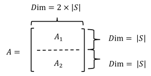
3.3.2. Totally Unimodular Property of the Coefficient Matrix for $n_s^{\mathrm{i}\mathrm{n}}$ and $n_s^{\mathrm{o}\mathrm{u}\mathrm{t}}$

A key strategy for efficiently solving large-scale optimization problems involves relaxing binary or integer variables into continuous ones without compromising the integrity of the solution. Within our proposed framework, the structure of constraints related to vessel chartering is of particular interest. By examining the mathematical properties of the corresponding coefficient matrix, we can identify conditions that permit such a relaxation, thereby enhancing the model’s tractability while preserving solution validity.

The TU property holds considerable significance in Integer Linear Programming (ILP). It enables the dropping of integer constraints without compromising optimality, thereby simplifying the solution process [51]. In practical scenarios, an ILP problem, which is generally NP-hard, can be solved efficiently through simpler LP techniques that work in polynomial time. This makes the TU property highly valuable in applications like network flows, scheduling, and resource allocation, where the underlying matrices often naturally possess this characteristic.

We introduce the following theorem to formalize this property for the variables $n_s^{\mathrm{i}\mathrm{n}}$ and $n_s^{\mathrm{o}\mathrm{u}\mathrm{t}},\forall s\in S$.

Theorem 3.

For all  $s$in$S$, the coefficient matrices of  $n_s^{\mathrm{i}\mathrm{n}}$ and $n_s^{\mathrm{o}\mathrm{u}\mathrm{t}}$ are TU.

The proof of Theorem 3 is presented in Appendix A.2. Combining Theorem 3 with the fact that the right-hand-side terms of constraints (1-4) and (1-5) are always integral allows for the relaxation of the integer variables $n_s^{\mathrm{i}\mathrm{n}}$and $n_s^{\mathrm{o}\mathrm{u}\mathrm{t}}$ to be continuous. The integrality of the right-hand side is assured, as these terms are constructed solely from the integer variables $n_{sr},\forall s\in S, \forall r\in R$ and the integer parameters $A_s, \forall s\in S$. The direct consequence of this relaxation is a significant reduction in the model’s computational burden, achieved without compromising the optimality of the solution.

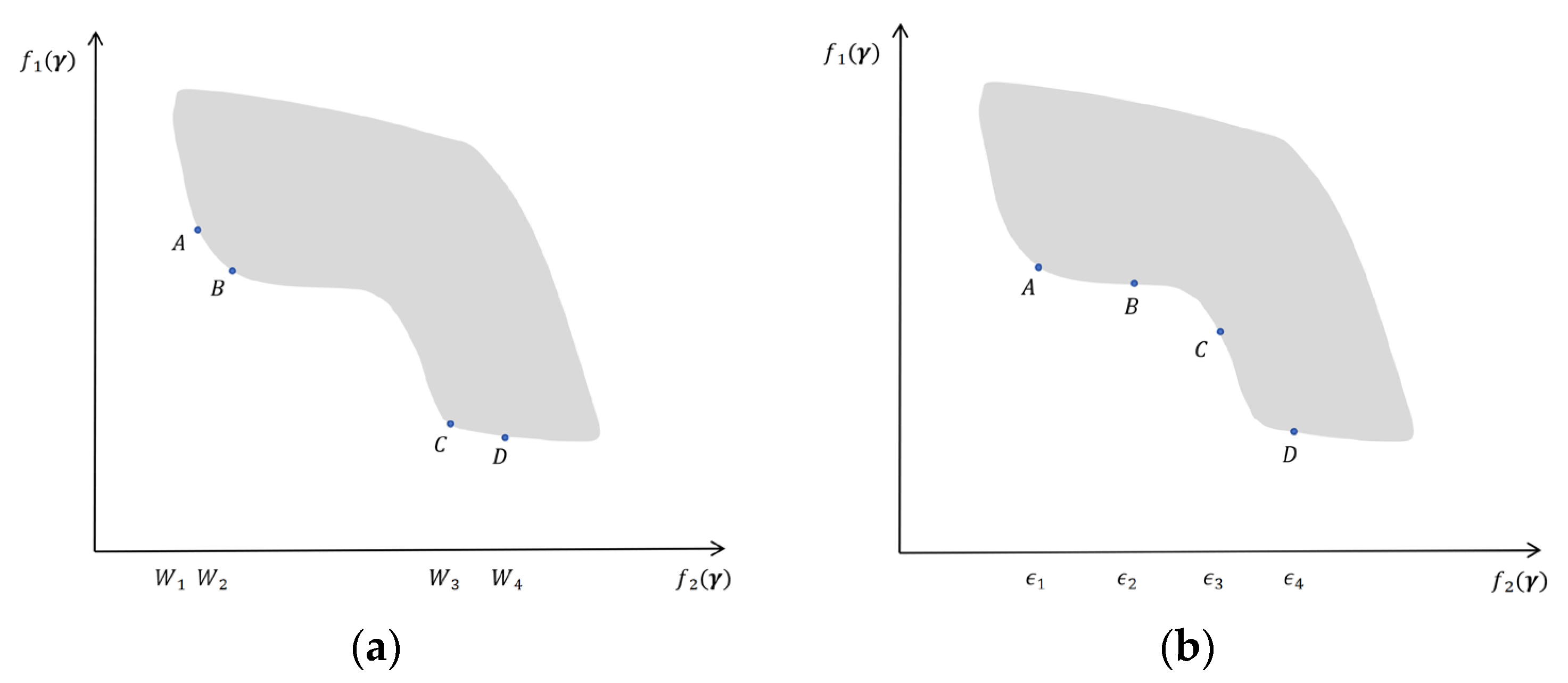
3.3.3. Structural Properties of the Pareto Frontier

To understand the structure of trade-offs between weekly profit and transport volume, it is essential to analyze the mathematical characteristics of the Pareto frontier generated by the bi-objective MIP model. Unlike single-objective models, bi-objective optimization yields a set of non-dominated solutions rather than a unique optimum. The following theorem characterizes the geometric and continuity properties of the Pareto frontier, providing foundational understanding for both theoretical analysis and algorithmic development.

Theorem 4.

The Pareto frontier consists of a finite union of line segments, and within each segment, the Pareto frontier is continuous and piecewise linear.

Theorem 5.

The Pareto frontier is generally non-convex and exhibits discontinuities.

The proofs of Theorems 4 and 5 are presented in Appendix A.3. This structure, which is non-convex and exhibits discontinuities due to distinct integer configurations, is illustrated in Figure 3, which provides a visual representation of the disconnected Pareto frontier. Each colored segment corresponds to the subset of solutions in the Pareto frontier under a fixed-integer configuration.

3.3.4. Diminishing Returns Within Local Pareto Segments

While the global Pareto frontier of the bi-objective model is composed of disconnected, non-convex segments arising from distinct integer configurations (as shown in Theorems 4 and 5), each individual segment associated with a fixed configuration exhibits a more regular structure. In particular, when integer decisions are held constant, the remaining problem reduces to a linear program over continuous variables, whose Pareto-efficient outcomes form a convex and piecewise-linear frontier. Within such a local segment, the trade-off between the two objectives intensifies progressively: improving one objective further requires increasingly larger sacrifices in the other. This structural property is formally characterized below.

Theorem 6.

The local Pareto frontier under a fixed-integer configuration becomes progressively steeper, indicating an increasing marginal rate of substitution between the two objectives.

The proof of Theorem 6 is presented in Appendix A.4.

4. Solving Method

4.1. Bi-Objective Optimization

Consider a bi-objective maximization problem formulated as follows:

$$\left\{\begin{array}{c}\underset{\mathit{g}\in G}{\mathrm{m}\mathrm{a}\mathrm{x}}{f}_1(\mathit{g})\\ \underset{\mathit{g}\in G}{\mathrm{m}\mathrm{a}\mathrm{x}}{f}_2(\mathit{g}),\end{array}\right.$$

(2)

where the solution $\mathit{g}$ belongs to a non-empty, compact set $G$. The two objective functions, $f_1\left(\mathit{g}\right)$ and $f_2\left(\mathit{g}\right)$, are upper semi-continuous functions to be maximized over this set. These objectives can be represented by a single objective vector $\mathit{f}\left(\mathit{g}\right)={\left(f_1\left(\mathit{g}\right),f_2\left(\mathit{g}\right)\right)}^{\mathrm{T}}$. Any such vector generated by a solution $\mathit{g}\in G$ is termed a feasible objective vector. The universe of all such achievable outcomes is the set $\mathbb{Y}=\left\{{\left(f_1\left(\mathit{g}\right),f_2\left(\mathit{g}\right)\right)}^{\mathrm{T}}|\mathit{g}\in G\right\}$. Within this framework, the goal is to identify Pareto-optimal solutions. A feasible solution $\mathit{g}$ is designated as Pareto optimal if it generates a non-dominated objective vector. A vector $\overline{\mathit{f}}\left(\mathit{g}\right)\in \mathbb{Y}$ is defined as non-dominated if no other feasible vector in $\mathbb{Y}$ offers a superior outcome. Specifically, there exists no other vector that is at least as good in all objectives (i.e., $f_i\left(\mathit{g}\right)>\overline{f_i}\left(\mathit{g}\right)$ for $i=1, 2$) and strictly better in at least one objective (i.e., $f_i\left(\mathit{g}\right)>\overline{f_i}\left(\mathit{g}\right)$ for some $i$). This definition aligns with the principle that a Pareto-optimal solution cannot be improved with respect to one objective without a simultaneous degradation in at least one of the others [52]. The locus of all such Pareto-optimal solutions, formally described by the set $\Psi =\left\{\mathit{g}\in G|\left(f_1\left(\mathit{g}\right),f_2\left(\mathit{g}\right)\right)\in \mathbb{Y}\right\}$, is designated as the Pareto frontier.

In previous research, the weighted sum method has been one of the most extensively applied approaches for addressing the multi-objective optimization problem of marine shipping route planning and ship allocation (e.g., [53,54,55]). This method aggregates multiple objectives, such as navigation risk, fuel consumption, travel time, and operational costs, into a single objective function by assigning specific weights to each objective. These weights reflect the relative importance of each objective and are typically determined through expert judgment, as exemplified by standardized allocations of 0.4 for risk, 0.3 for fuel consumption, and 0.3 for travel time in one study [53]. Alternatively, weights may be derived using systematic techniques such as the Analytic Hierarchy Process (AHP) combined with entropy-based methods to ensure robustness in complex scenarios like Arctic rescue operations [54]. In some cases, weights are dynamically adjusted during algorithm execution, accompanied by sensitivity analysis to assess their impact on the solution, as seen in hub-and-spoke network optimization for short sea shipping [55].

The weighted sum method is advantageous due to its simplicity, as it allows for an easy assessment of the trade-offs between different objectives based on assigned weights. It also facilitates the interaction between decision makers’ subjective preferences and the system’s objective information through the adjustment of the weight combinations for various objective functions. Nevertheless, this approach has certain limitations when applied to multi-objective optimization problems. As an a priori technique, it necessitates predetermined weights for each objective function, meaning that the optimal result obtained is heavily dependent on these assigned weights. Therefore, when the relative importance of each objective is uncertain or cannot be established beforehand, which is common in hazardous waste management system planning due to the complexity of balancing environmental risks, economic costs, and social impacts, the weighted sum method becomes less effective. In the context of a posteriori decision making, Das and Dennis [56] noted that it cannot produce a well-distributed set of Pareto solutions or a comprehensive array of points along the Pareto frontier. An example shown in Figure 4 of this study demonstrates that the weighted sum method is unable to identify the Pareto frontier within a non-convex feasible region, with their work providing further details about the method’s limitations.

4.2. The Augmented $ϵ$-Constraint Method

Given the limitations of the weighted sum method, especially in scenarios where objective importance is unclear or in a posteriori decision making, it becomes necessary to explore alternative approaches. As an a posteriori method, the $ϵ$-constraint method has been extensively employed in the literature for approximating the Pareto frontier in multi-objective problems [52]. In this approach, one objective is selected as the primary goal, with the remaining objectives reformulated as constraints. However, identifying extreme value points typically requires sorting, expansion, and compression steps, which are time-consuming and make it difficult to estimate the maximum attainable value of the objective to be maximized. To address the bi-objective MIP model, we utilize the augmented $ϵ$-constraint approach, which enhances the standard method by adding a penalty term to the objective function. This innovation brings multiple key advancements over classical $ϵ$-constraint techniques. In contrast to the basic $ϵ$-constraint method, which often generates weakly efficient solutions that allow one objective function to be improved while keeping the other objective functions unaffected, the augmented $ϵ$-constraint method effectively eliminates such weak solutions by integrating both objectives into a single penalized objective function. Specifically, non-Pareto-optimal solutions require manual removal through pairwise comparisons. The augmented approach integrates both objectives into a single optimized function, inherently filtering out non-Pareto-optimal candidates during computation and eliminating the need for post-processing steps. Additionally, the penalty term’s design allows dynamic adjustment of the tolerance level $ϵ$, enabling more flexible and precise control over solution density. For instance, when objective functions take integer values, setting $ϵ<1$ ensures the augmented method captures the full set of non-dominated objective vectors, making it particularly suitable for complex scenarios like transportation route optimization where fine-grained management of trade-offs between objectives (such as time and risk) is critical [57]. This improvement not only helps to better manage infeasible solutions but also accelerates convergence toward the Pareto frontier. Moreover, compared with traditional $ϵ$-constraint variants (such as the revised or improved revised methods) that require solving two separate single-objective models for each iteration, the augmented method achieves equivalent results with only one model, significantly reducing redundant calculations and boosting computational efficiency. Overall, this approach effectively balances solution quality and computational efficiency while maintaining the theoretical rigor of Pareto optimality. The augmented $ϵ$-constraint method is elaborated as follows.

Based on the bi-objective optimization model (2), let $f_1^{\mathrm{m}\mathrm{a}\mathrm{x}}:=\underset{\mathit{g}\in G}{\mathrm{m}\mathrm{a}\mathrm{x}}{f}_1(\mathit{g})$ and $f_2^{\mathrm{m}\mathrm{a}\mathrm{x}}:=\underset{\mathit{g}\in G}{\mathrm{m}\mathrm{a}\mathrm{x}}{f}_2(\mathit{g})$. Let $f_1^{\mathrm{m}\mathrm{i}\mathrm{n}}:=\underset{\mathit{g}\in G}{\mathrm{m}\mathrm{a}\mathrm{x}}{f}_1(\mathit{g})$ subject to $f_2(\mathit{g})\ge f_2^{\mathrm{m}\mathrm{a}\mathrm{x}}$, $\mathit{g}\in G$. Let $ϵ$ be a small positive number such that $f_1^{\mathrm{m}\mathrm{a}\mathrm{x}}-f_1^{\mathrm{m}\mathrm{i}\mathrm{n}}$ is an integer multiple of $ϵ$. Define a multiset $\mathsf{\Omega }:=\mathrm{\varnothing }$, where $\mathsf{\Omega }$ represents a multiset composed of obtained solutions by the augmented $ϵ$-constraint method. Define $K$ as the parameter that determines the maximum number of iterations in the subsequent iterative process. It essentially quantifies how many discrete steps can be taken based on the chosen $ϵ$. $K:=\left(f_1^{\mathrm{m}\mathrm{a}\mathrm{x}}-f_1^{\mathrm{m}\mathrm{i}\mathrm{n}}\right)/ϵ$. Set $k\leftarrow K$ where $k$ is an iteration counter initializing to the value of $K$. In each iteration of the algorithm, the value of $k$ will be updated based on the results of the optimization in that iteration. We solve the following single-objective optimization model:

$$\mathrm{m}\mathrm{a}\mathrm{x}\left\{f_2\left(\mathit{g}\right)+ϵ{\displaystyle \frac{f_1\left(\mathit{g}\right)-f_1^{\mathrm{m}\mathrm{i}\mathrm{n}}}{f_1^{\mathrm{m}\mathrm{a}\mathrm{x}}-f_1^{\mathrm{m}\mathrm{i}\mathrm{n}}}}\right\}$$

(3)

subject to

$$f_1\left(\mathit{g}\right)\ge f_1^{\mathrm{m}\mathrm{i}\mathrm{n}}+kϵ, \mathit{g}\in G,$$

(4)

Then, we let $\dot{\mathit{g}}\left(k\right)$ be an optimal solution obtained by (2) and $\mathsf{\Omega }\leftarrow \mathsf{\Omega }\cup \left\{\dot{\mathit{g}}\left(k\right)\right\}$ in each iteration. Let $\widehat{k}$ be the largest integer satisfying $f_1^{\mathrm{m}\mathrm{i}\mathrm{n}}+\widehat{k}ϵ<f_1\left(\dot{\mathit{g}}\left(k\right)\right)$. If $\widehat{k}<0$, return $\mathsf{\Omega }$ and stop. Conversely, if $\widehat{k}\ge 0$, we update the value of $k$ by $k\leftarrow \widehat{k}$. Then, the procedure of solving (2) is repeated. This iterative process continues until $\widehat{k}<0$, gradually refining and expanding the set of optimal solutions stored in $\mathsf{\Omega }$. Through this iterative mechanism, the algorithm systematically explores the solution space of the bi-objective optimization problem, aiming to converge at the Pareto-optimal set. Compared to classical scalarization techniques, this method provides a balance between exploration and efficiency by embedding trade-off control directly into the objective function and requiring only one model to be solved per iteration, making it especially suitable for large-scale or computation-intensive bi-objective optimization problems.

The pseudocode for the augmented $ϵ$-constraint method is shown in Algorithm 1.

Algorithm 1 Augmented $ϵ$-constraint method

1: Calculate $f_1^{\mathrm{m}\mathrm{a}\mathrm{x}}=\underset{\mathit{g}\in G}{\max }{f}_1\left(\mathit{g}\right)$ 2: Calculate $f_2^{\mathrm{m}\mathrm{a}\mathrm{x}}=\underset{\mathit{g}\in G}{\max }{f}_2\left(\mathit{g}\right)$ 3: Calculate $f_1^{\mathrm{m}\mathrm{i}\mathrm{n}}=\mathrm{m}\mathrm{a}\mathrm{x}{f}_1\left(\mathit{g}\right)$ subject to $f_2\left(\mathit{g}\right)\ge f_2^{\mathrm{m}\mathrm{i}\mathrm{n}}$, $\mathit{g}\in G$ 4: $ϵ\leftarrow$a small positive number such that $f_1^{\mathrm{m}\mathrm{a}\mathrm{x}}-f_1^{\mathrm{m}\mathrm{i}\mathrm{n}}$ is an integer multiple of $ϵ$ 5: $k\leftarrow \left(f_1^{\mathrm{m}\mathrm{a}\mathrm{x}}-f_1^{\mathrm{m}\mathrm{i}\mathrm{n}}\right)/ϵ$ 6: $\dot{\mathit{g}}\left(k\right)\leftarrow \mathrm{n}\mathrm{u}\mathrm{l}\mathrm{l}$ 7: $\mathsf{\Omega }\leftarrow \mathrm{\varnothing }$ 8: $\widehat{k}\leftarrow 0$ 9: while $\widehat{k}\ge 0$ do 10: Solve the model $\left(14\right)$, and obtain an optimal solution $\dot{\mathit{g}}\left(k\right)$. 11: $\mathsf{\Omega }\leftarrow \mathsf{\Omega }\cup \left\{\dot{\mathit{g}}\left(k\right)\right\}$ 12: Calculate the largest integer $\widehat{k}$ satisfying $f_1^{\mathrm{m}\mathrm{i}\mathrm{n}}+\widehat{k}ϵ<f_1\left(\dot{\mathit{g}}\left(k\right)\right)$. 13: $k\leftarrow \widehat{k}$ 14: end while 15: Return $\mathsf{\Omega }$.

5. Experiments

To validate the performance of our proposed model, this section presents a series of computational experiments. All numerical tests were conducted on a desktop equipped with a 13th Generation Intel Core i7 CPU and 32 GB of RAM. All codes are computed in Python (version 3.11.5) and the mathematical models are solved by Gurobi (version 10.0.1). The experiment section contains mainly two parts: a case study based on the real shipping network, where we established a baseline of results by assigning initial values to the model’s parameters, and detailed sensitivity analyses on critical parameters, through which we systematically investigate how variations in these parameters influence the outcomes.

5.1. Experiment Settings

The parameters are divided into three categories as follows:

• Ship-Type-Related Parameters. Three ship capacities (12,000-TEU, 15,000-TEU, and 20,000-TEU) and two types of countries of construction (China and other countries) are considered, resulting in six distinct ship types. The weekly charter-in prices $c_s^{\mathrm{i}\mathrm{n}}$ for the 12,000-TEU, 15,000-TEU, and 20,000-TEU ships are set at 0.6 million USD, 0.7 million USD, and 1 million USD, respectively. The corresponding charter-out prices $c_s^{\mathrm{o}\mathrm{u}\mathrm{t}}$ are fixed at 80% of the charter-in prices, i.e., $c_s^{\mathrm{o}\mathrm{u}\mathrm{t}}=0.8c_s^{\mathrm{i}\mathrm{n}}$. Based on operational data detailing the CMA CGM‘s owned fleet deployed in Asia, Europe, and North America [58,59,60,61], and in line with reports indicating that and 64% of its newbuilding capacity was on order at Chinese yards [62], we consider 15 China-built 12,000-TEU ships, 25 China-built 15,000-TEU ships, 41 China-built 20,000-TEU ships, 10 non-China-built 12,000-TEU ships, 13 non-China-built 15,000-TEU ships, and 23 non-China-built 20,000-TEU ships. The specific technical parameters corresponding to these six categories are presented in

  Table 2. The parameters for the six types of ships.

  ID	Countries of Construction	${\mathit{Q}}_{\mathit{s}}$(TEUs)	${\mathit{c}}_{\mathit{s}}^{\mathbf{i}\mathbf{n}}$ (Million USD)	${\mathit{c}}_{\mathit{s}}^{\mathbf{o}\mathbf{u}\mathbf{t}}$ (Million USD)	${\mathit{A}}_{\mathit{s}}$
  1	China	12,000	0.6	0.48	15
  2	China	15,000	0.7	0.56	25
  3	China	20,000	1.0	0.80	41
  4	Other countries	12,000	0.6	0.48	10
  5	Other countries	15,000	0.7	0.56	13
  6	Other countries	20,000	1.0	0.80	23

  .
• Rout-Related Parameters. In this study, we select 20 candidate routes, including their ports of call and the corresponding number of ships required to ensure a weekly departure frequency on each operated route [62,63,64,65,66,67,68]. The routes and their weekly departure frequencies are detailed in

  Table 3. The parameters for the 20 routes.

  ID	${\mathit{N}}_{\mathit{r}}$	$\mathbf{Ports} \mathbf{of} \mathbf{Call}$	Includes U.S. Port
  1	9	Qingdao → Shanghai → Ningbo → Xiamen → Yantian → Singapore → Felixstowe → Zeebrugge → Gdynia → Wilhelmshaven → Singapore → Yantian → Qingdao	No
  2	8	Tianjin → Dalian → Qingdao → Shanghai → Ningbo → Singapore → Rotterdam → Hamburg → Antwerp → Shanghai → Tianjin	No
  3	9	Qingdao → Ningbo → Yantian → Tanjung Pelepas → Antwerp → Gdynia → Gdansk → Klaipeda → King Abdullah Port → Singapore → Qingdao	No
  4	15	Yokohama → Busan → Shanghai → Ningbo → Yantian → Hong Kong → Singapore → Port Klang → Laem Chabang → Haiphong → Manila → Kaohsiung → Suez Canal → Piraeus → Valencia → Barcelona → Genoa → Salerno → Naples → Gioia Tauro → Istanbul → Alexandria → Algeciras → Suez Canal → Chennai → Tanjung Pelepas → Yokohama	No
  5	9	Yokohama → Tokyo → Kobe → Nagoya → Busan → Kaohsiung → Singapore → Suez Canal → Piraeus → Valencia → Barcelona → Suez Canal → Singapore → Yokohama	No
  6	6	Singapore → Suez Canal → Genoa → Rotterdam → Hamburg → Antwerp → Suez Canal → Singapore	No
  7	9	Hamburg → Rotterdam → Antwerp → Le Havre → Felixstowe → Gdansk → Oslo → Copenhagen → Stockholm → Piraeus → Barcelona → Genoa → Valencia → Salerno → Naples → Istanbul → Alexandria → Algeciras → Haifa → Hamburg	No
  8	4	Hamburg → Rotterdam → Antwerp → Le Havre → Piraeus → Barcelona → Genoa → Valencia → Hamburg	No
  9	9	Tokyo → Shimizu → Kobe → Nagoya → Singapore → Suez Canal → Damietta → Rotterdam → Hamburg → Le Havre → Suez Canal → Singapore → Tokyo	No
  10	8	Busan → Tanjung Pelepas → Southampton → Le Havre → Hamburg → Rotterdam → Port Klang → Busan	No
  11	8	Southampton → Antwerp → Rotterdam → Bremerhaven → Le Havre → New York → Norfolk → Baltimore → Southampton	Yes
  12	6	Antwerp → Rotterdam → Bremerhaven → Liverpool → Newark → Savannah → Everglades → North Charleston → Antwerp	Yes
  13	9	Laem Chabang → Singapore → Colombo → Suez Canal → Halifax → New York → Savannah → Jacksonville → Norfolk → Halifax → Suez Canal → Jebel Ali → Singapore → Laem Chabang	Yes
  14	9	Busan → Gwangyang → Shanghai → Xiamen → Yantian → Hong Kong → Tanjung Pelepas → Singapore → Jakarta → Surabaya → Jakarta → Tanjung Pelepas → Singapore → Subic → Manila → Kaohsiung → Tokyo → Busan	No
  15	9	Penang → Singapore → Laem Chabang → Danang → Busan → Long Beach → Oakland → Yokohama → Ningbo → Shanghai → Xiamen → Yantian → Singapore → Penang	Yes
  16	8	Danang → Haiphong → Yantian → Ningbo → Shanghai → Qingdao → Busan → Seattle → Prince Rupert → Vancouver → Busan → Danang	Yes
  17	6	Haiphong → Xiamen → Nansha → Yantian → Los Angeles → Haiphong	Yes
  18	6	Qingdao → Shanghai → Ningbo → Los Angeles → Oakland → Busan → Qingdao	Yes
  19	8	Haiphong → Yantian → Ningbo → Shanghai → Seattle → Los Angeles → Yokohama → Xiamen → Haiphong	Yes
  20	7	Xingang → Qingdao → Gwangyang → Ningbo → Yantian → Tanjung Pelepas → Algeciras → Bremerhaven → Xingang	No

  .
• Transport-Related Parameters. We select a set of OD pairs and estimate the pairs’ weekly transport demand $D_{od}$ for each OD pair. To ensure these estimations are grounded in realistic market conditions, they are carefully calibrated. This calibration is based on aggregated containerized cargo flow data from [69] and insights into global shipping trends from [70], ensuring that the demand volumes and their distribution are representative of actual trade patterns. The weekly transport demand of these OD pairs $D_{od}$ are detailed in

  Table 4. The weekly transport demands of the OD pairs.

  ID	$\mathbf{(}\mathit{o},\mathit{d}\mathbf{)}$	${\mathit{D}}_{\mathit{o}\mathit{d}}$ (TEUs/Week)	ID	$\mathbf{(}\mathit{o},\mathit{d}\mathbf{)}$	${\mathit{D}}_{\mathit{o}\mathit{d}}$ (TEUs/Week)
  1	(Shanghai, Rotterdam)	35,000	31	(Nagoya, Rotterdam)	10,500
  2	(Ningbo, Felixstowe)	28,000	32	(Shimizu, Hamburg)	7000
  3	(Ningbo, Antwerp)	28,000	33	(Laem Chabang, Savannah)	7000
  4	(Shanghai, Piraeus)	21,000	34	(Singapore, Jacksonville)	10,500
  5	(Yantian, Barcelona)	14,000	35	(Colombo, Halifax)	3500
  6	(Yokohama, Piraeus)	3500	36	(Rotterdam, Savannah)	17,500
  7	(Busan, Valencia)	2800	37	(Bremerhaven, Newark)	17,500
  8	(Singapore, Genoa)	4200	38	(Liverpool, Everglades)	14,000
  9	(Kaohsiung, Barcelona)	2450	39	(Antwerp, North Charleston)	17,500
  10	(Port Klang, Salerno)	1750	40	(Tanjung Pelepas, Gdansk)	10,500
  11	(Laem Chabang, Istanbul)	1400	41	(Antwerp, Klaipeda)	14,000
  12	(Haiphong, Gioia Tauro)	1750	42	(Gdynia, King Abdullah Port)	7000
  13	(Manila, Algeciras)	1050	43	(Busan, Tokyo)	7000
  14	(Hamburg, Piraeus)	5600	44	(Singapore, Tokyo)	10,500
  15	(Rotterdam, Barcelona)	7000	45	(Xiamen, Kaohsiung)	14,000
  16	(Antwerp, Genoa)	4900	46	(Yantian, Subic)	10,500
  17	(Le Havre, Valencia)	4200	47	(Hong Kong, Jakarta)	14,000
  18	(Felixstowe, Istanbul)	2800	48	(Tanjung Pelepas, Surabaya)	7000
  19	(Gdansk, Alexandria)	2100	49	(Singapore, Manila)	10,500
  20	(Oslo, Naples)	1400	50	(Manila, Kaohsiung)	7000
  21	(Copenhagen, Algeciras)	2450	51	(Long Beach, Shanghai)	2300
  22	(Stockholm, Haifa)	1750	52	(Shanghai, Seattle)	5500
  23	(Tokyo, Rotterdam)	10,500	53	(Ningbo, Seattle)	3800
  24	(Busan, Rotterdam)	14,000	54	(Busan, Seattle)	2000
  25	(Singapore, Rotterdam)	17,500	55	(Xiamen, Los Angeles)	8000
  26	(Rotterdam, New York)	21,000	56	(Ningbo, Los Angeles)	10,000
  27	(Antwerp, New York)	21,000	57	(Ningbo, Bremerhaven)	5000
  28	(Le Havre, New York)	17,500	58	(Yantian, Algeciras)	4000
  29	(Colombo, New York)	7000	59	(Tanjung Pelepas, Bremerhaven)	3500
  30	(Kobe, Rotterdam)	10,500	60	(Xingang, Bremerhaven)	3700

  . The involved ports are classified into three geographic regions: East Asia and Southeast Asia, Europe and the Mediterranean, and North America. Based on [71,72,73] we further estimate the freight rate per transported TEU for each OD pair, which is detailed in

  Table 5. Profit parameters of OD pairs.

  ID	Origin	Destination	${\mathit{p}}_{\mathit{o}\mathit{d}}$ (USD/TEU)
  1	East Asia and Southeast Asia	Europe and the Mediterranean	1101
  2	Europe and the Mediterranean	East Asia and Southeast Asia	232
  3	East Asia and Southeast Asia	North America	1445
  4	North America	East Asia and Southeast Asia	1295
  5	North America	Europe and the Mediterranean	421
  6	Europe and the Mediterranean	North America	1021
  7	East Asia and Southeast Asia	East Asia and Southeast Asia	353
  8	Europe and the Mediterranean	Europe and the Mediterranean	250
  9	North America	North America	1500

  .

All ships use very low-sulfur fuel oil (VLSFO). Referring to [74], the daily consumption (ton/day) of ships of type $s$ sailing on route $r$ at speed $v$ is expressed as follows:

$$f_{sr}\left(v\right)=a_{sr}·v^{b_{sr}},$$

(5)

where $a_{sr}$ and $b_{sr}$ are parameters related to ship types and sea conditions on the route. The fuel cost parameters for ships with different capacities are presented in

Table 6. The fuel cost parameters for ships of different capacities.

${\mathit{Q}}_{\mathit{s}}$ (TEUs)	${\mathit{a}}_{\mathit{s}\mathit{r}}$	${\mathit{b}}_{\mathit{s}\mathit{r}}$
12,000	0.01210	2.947
15,000	0.00433	3.314
20,000	0.02420	2.914

, with $a_{sr}$ and $b_{sr}$ derived from the median of the value ranges provided in [74].

The sailing speed is uniformly set to $v=20$ knots. The round-trip time required for one ship to complete the full loop at speed $v$ is denoted by $t_r$ (weeks), which is numerically equal to $N_r$. Thus, the fuel cost of one ship of type $s$ completing one full trip on route $r$ is calculated by $F_{sr}=7t_r·c_f·f_{sr}\left(v\right)$, where $c_f$ is the unit fuel price, set as 574 USD/ton based on global bunker prices [75].

The berthing cost for one ship of type $s$ per port visit is denoted by $c_s^{\mathrm{b}\mathrm{e}\mathrm{r}\mathrm{t}\mathrm{h}}$, specifically 0.3 million USD, 0.4 million USD, and 0.5 million USD for the 12,000-TEU, 15,000-TEU, and 20,000-TEU ships, respectively. Given the number of ports visited on route $r$ (denoted by $P_r$), the berthing cost for a ship of type $s$ for a full round trip on route $r$ is calculated as $B_{sr}=c_s^{\mathrm{b}\mathrm{e}\mathrm{r}\mathrm{t}\mathrm{h}}·P_r$.

The extra penalties specifically incurred by China-built ships when deployed on routes calling at U.S. ports are based on [50]. Specifically, only China-built ships with capacities above 4000 TEUs incur an extra fee of 120 USD/TEU per rotation or per string of U.S. port calls. China-built ships below 4000 TEUs and ships built in other countries are exempt from this fee when calling at U.S. ports. As all China-built ship types considered in this study have capacities exceeding 4000 TEUs; they are all subject to this extra fee when sailing on routes which include U.S. port calls.

After establishing the parameter settings, we use these values to derive the basic results, and then we conduct a sensitivity analysis on a key parameter.

5.2. Basic Results

This section presents the detailed basic results derived from the proposed bi-objective MIP model using the augmented $ϵ$-constraint method, with $ϵ=\left(f_1^{\mathrm{m}\mathrm{a}\mathrm{x}}-f_1^{\mathrm{m}\mathrm{i}\mathrm{n}}\right)/20$. Section 5.2.1 provides a comprehensive bi-objective optimization analysis, during which three representative Pareto-optimal solutions were identified along the Pareto frontier. Section 5.2.2 analyzes these three Pareto-optimal solutions in terms of route operation strategy, ship charter strategy, and route assignment, as well as transport demand assignment.

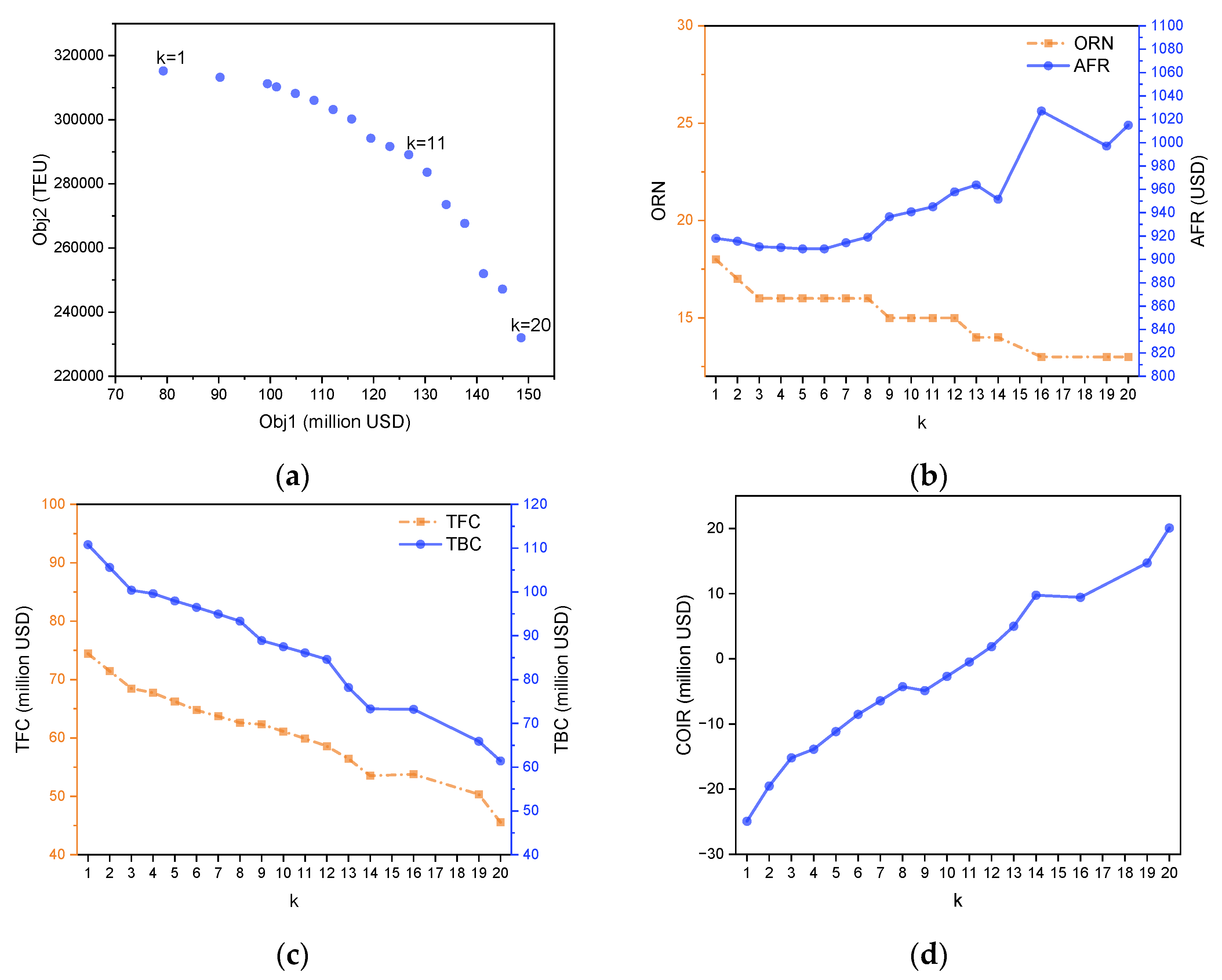
5.2.1. Bi-Objective Optimization Results Analysis

Figure 5 shows the optimal results of the bi-objective MIP model. Figure 5a shows the Pareto frontier, with the x-axis representing the total weekly profit (Obj 1) and the y-axis representing the total weekly transport volume (Obj 2). In Figure 5b–d, the x-axis represents $k$, tracking increasing values of Obj 1. The y-axis of Figure 5b–d corresponds to the values of indicators, including the number of operated routes (ORN) and the average freight rate (AFR) of accepted transport demand, the total fuel cost (TFC) and the total berthing cost (TBC) of all ships, and the revenue from chartering out idle ships minus the cost of chartering in ships (COIR).

The Pareto frontier depicted in Figure 5a demonstrates the inherent trade-off between Obj 1 and Obj 2. The Pareto frontier provides a powerful decision-making reference for shipping managers by revealing two distinct layers of choice. The first layer concerns major strategic decisions. For a shipping company, these correspond to discrete, high-impact actions, for example, activating an entire service route or reallocating a specific ship type. This structure indicates that when the company wants to pursue one objective significantly, such as substantially increasing profit, it must make these major adjustments to its route operations and fleet deployment. This is fundamentally different from making small-scale adjustments to accepted cargo while the network structure remains fixed. In situations where only minor fine-tuning between profit and transport volume is desired, keeping the activated routes and deployed ships constant while adjusting cargo acceptance is the more effective strategy. This clear distinction between major structural changes and minor operational adjustments provides a practical validation of Theorem 5, which establishes that the frontier’s overall structure is fundamentally determined by the integer decision variables governing the network design. At the operational level, within each of these fixed strategic configurations, the convex shape of the frontier illustrates the law of diminishing returns. For a shipping manager, this signifies that pushing for an extreme on one objective comes at a disproportionately high cost to the other. This phenomenon of a progressively steepening trade-off is formally established in Theorem 6. Therefore, the frontier serves as a practical guide for finding the optimal trade-off based on current corporate priorities. For instance, if the primary goal is to expand market share, a decision maker would select a solution from the frontier that prioritizes higher transport demand acceptance. Conversely, if the immediate need is to improve profitability and strengthen cash flow, a solution yielding higher profit would be chosen, even at the expense of some volume. The frontier quantifies these choices, enabling managers to make informed decisions that align their network strategy with their most pressing business objectives.

Figure 5b shows that ORN decreases as Obj 1 increases. This reduction in ORN enables the company to concentrate resources on the most profitable transport services rather than dispersing them across marginally profitable ones. The strategic elimination of less profitable routes directly contributes to cost reduction and operational efficiency. This cost reduction is clearly demonstrated in Figure 5c, where both TFC and TBC decrease as Obj 1 increases. Simultaneously, AFR rises from approximately 900 USD/TEU to 1000 USD/TEU as Obj 1 increases, demonstrating that the company prioritizes transport demand with high $p_{od}$ (such as from Asia to North America) while rejecting lower-value shipments (such as from Europe to Asia). This selective approach to transport demand acceptance significantly reduces transport cost and increases the total profit.

Figure 5d illustrates the COIR increases as Obj 1 increases, indicating that the fleet size required diminishes as ORN decreases. As accepted transport demand decreases, more ships become available for chartering out. The combination of reduced charter-in costs and increased charter-out revenue creates a substantial positive impact on profitability.

Table 7. Pareto-optimal solutions of the bi-objective MIP model.

$\mathit{k}$	Obj 1 (Million USD)	Obj 2 (TEUs)	ORN	AFR (USD)	TFC (Million USD)	TBC (Million USD)	The Extra Penalty Cost	COIR (Million USD)
1	79.26	315,250	18	918	74.44	110.79	0	−24.92
2	90.26	313,250	17	916	71.45	105.59	0	−19.52
3	99.44	311,250	16	911	68.46	100.39	0	−15.20
4	101.18	310,250	16	910	67.73	99.61	0	−13.88
5	104.84	308,217	16	909	66.24	97.95	0	−11.16
6	108.47	306,064	16	909	64.77	96.48	0	−8.52
7	112.16	303,203	16	914	63.69	94.94	0	−6.44
8	115.74	300,231	16	919	62.59	93.33	0	−4.28
9	119.47	294,231	15	937	62.32	88.89	0	−4.88
10	123.13	291,675	15	941	61.10	87.50	0	−2.68
11	126.80	289,120	15	945	59.87	86.10	0	−0.48
12	130.36	283,642	15	958	58.60	84.61	0	1.88
13	134.06	273,564	14	964	56.42	78.17	0	5.00
14	137.64	267,675	14	952	53.52	73.30	0	9.76
16	141.28	251,997	13	1027	53.77	73.20	0	9.44
19	144.96	247,189	13	997	50.34	65.90	0	14.72
20	148.58	232,016	13	1015	45.57	61.42	0	20.08

shows the optimal results of the model.

Notably, the extra penalty cost specifically incurred by China-built ships when deployed on routes calling at U.S. ports is equal to 0 in every Pareto-optimal solution, indicating that the model effectively avoids the extra penalty cost. The extra fee, amounting to 120 USD/TEU per rotation or per string of U.S. port calls for China-built ships with capacities above 4000 TEUs [50], is evidently substantial. Consequently, the model strategically assigns these China-built ships to routes excludes U.S. ports.

5.2.2. Representative Solutions Analysis

Based on the analysis of the Pareto frontier, three representative Pareto-optimal solutions are strategically selected for analysis in terms of route operation strategy, ship charter strategy, and route assignment, as well as transport demand assignment. These solutions, corresponding to $k$ = 1, $k$ = 11, and $k$ = 20, were chosen to capture distinct positions along the trade-off curve between maximizing Obj 1 and Obj 2. Specifically, the solution at $k$ = 1 represents a strategy characterized by the highest accepted transport demand among the non-dominated set. Conversely, the solution at $k$ = 20 corresponds to the highest total weekly profit. The solution at $k$ = 11 serves as an intermediate point, reflecting a balanced compromise between the competing objectives. The route operation strategy of the three selected optimal solutions is detailed in

Table 8. Route operation strategy of the selected Pareto-optimal solutions.

$\mathit{k}$	ID of Operated Routes	Total Number of Operated Routes
1	1–17, 20	18
11	1–4, 6, 8–14, 16, 17, 20	15
20	1–3, 6, 8–13, 16, 17, 20	13

.

Table 8 shows that the 13 routes selected for operation when $k=20$ are also part of the operational set for $k=1$ and $k=11$, indicating these routes are economically attractive, as the OD pairs on these routes offer higher freight rates or the ships deployed on these routes incur relatively lower transport costs.

Table 9. Ship charter and route assignment strategy.

$\mathit{k}$	The ID of Ship Types	ID of Assignment Routes	Charter in Quantity	Charter out Quantity
1	1	5, 10	0	4
	2	7, 10, 20	0	5
	3	1–4, 14	9	0
	4	15–17	13	0
	5	8	0	11
	6	6, 8, 9, 11–13, 20	19	0
11	1	10	0	13
	2	4, 10, 14	0	3
	3	1–3, 6, 8, 9	0	0
	4	16, 17	4	0
	5	4, 14, 20	0	0
	6	1, 11–14, 20	6	0
20	1	10, 20	0	8
	2	1, 10, 20	0	7
	3	2, 3, 6, 9	0	17
	4	16, 17	4	0
	5	8, 9	0	0
	6	11–13	0	0

details the ship charter and route assignment strategy for the three selected Pareto-optimal solutions. When $k=1$, the strategy prioritizes maximizing Obj 2. This is reflected in significant charter-in activity, particularly charting in 28 20,000-TEU ships, suggesting an effort to expand the average transport capacity of available fleet. Conversely, when $k=20$, the strategy prioritizes maximizing Obj 1. For this instance, 17 units of owned China-built 20,000-TEU ships (Type 3), 8 units of owned China-built 12,000-TEU ships (Type 1), and 7 units of owned China-built 15,000-TEU ships (Type 2) are chartered out. This indicates a smaller operational scale consistent with a profit-maximization approach.

A noteworthy pattern observed across all three Pareto-optimal solutions ($k=1$, 11, and 20) is the simultaneous chartering out of owned China-built 12,000-TEU ships (Type 1) and the chartering in of non-China-built ships of the same 12,000-TEU capacity (Type 4). For example, even at $k=1$, while pursuing maximum volume, 4 owned Type 1 ships are chartered out, and 13 Type 4 ships are chartered in. This consistent swap suggests a deliberate operational tactic to manage the fleet composition, likely to avoid the extra penalty cost associated with deploying specific ship types (China-built) on certain routes, by substituting them with exempt alternatives.

Table 10. Total volume of accepted transport demand and the average freight rate of the transported cargo.

$\mathit{k}$	Total Volume of Accepted Demand (TEU)	$\mathbf{Average} \mathbf{of} {\mathit{p}}_{\mathit{o}\mathit{d}}$ (USD)
1	315,250	918
11	289,120	945
20	232,016	1015

presents the total volume of accepted transport demand and the average freight rate of the transported cargo.

5.3. Sensitivity Analysis

By conducting sensitivity analysis experiments, we further analyze the sensitivity of our model to the changes in input parameters, including the freight rate, the surcharge intensity, the charter-in cost and charter-out revenue of ships, and the transport demand.

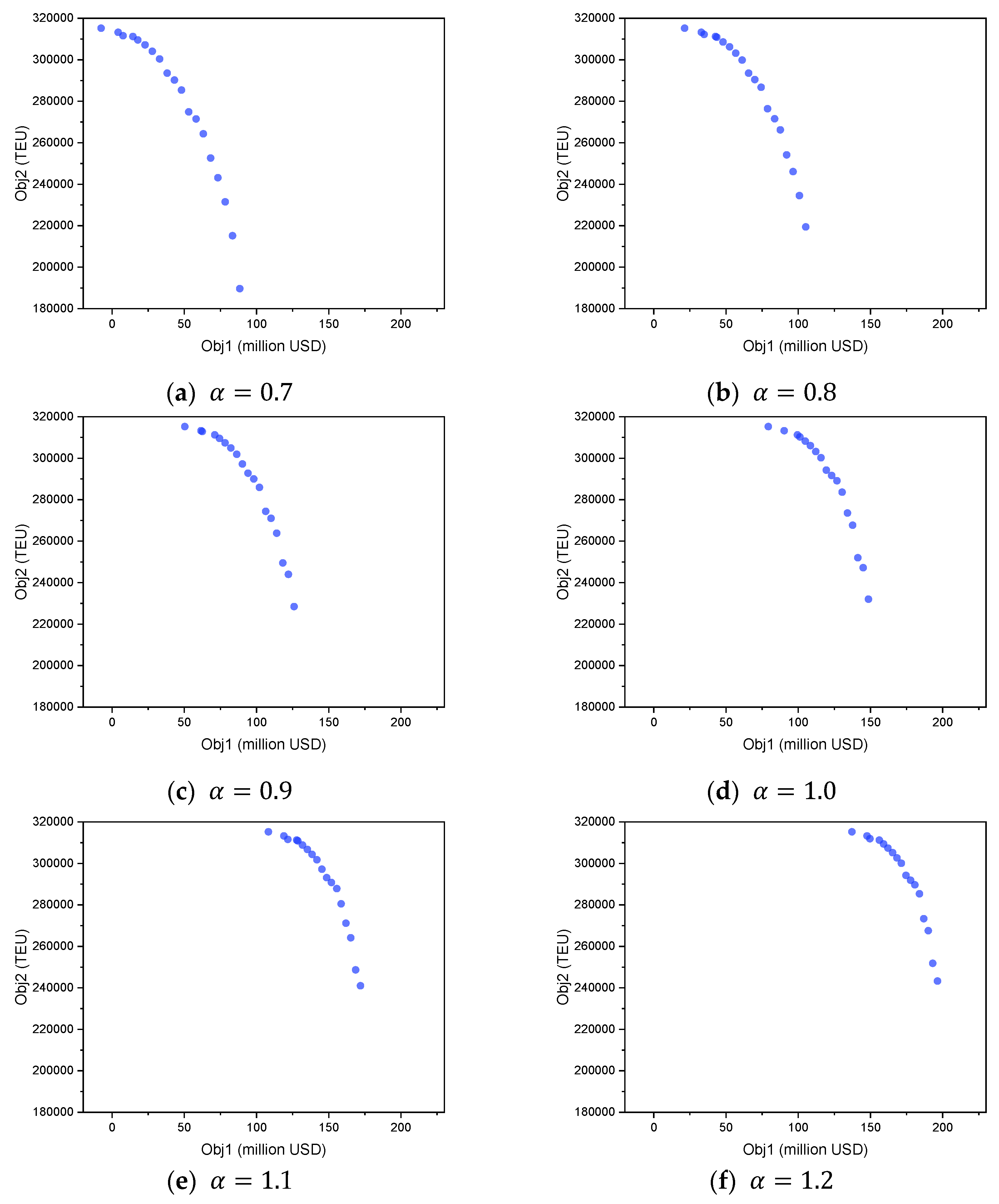
5.3.1. Sensitivity Analysis on the Freight Rate Ratio

In this section, we further analyze the sensitivity of our bi-objective MIP model to the changes in the freight rate per transported TEU. Generally, we conduct 6 experiments, aiming to illustrate the performance of the bi-objective MIP model in solving instances with different freight rate ratio. The ratio is denoted as $\alpha$, where the original freight rate is $p_{od}$, the actual freight rate is $p_{od}^{\mathrm{a}\mathrm{c}\mathrm{t}\mathrm{u}\mathrm{a}\mathrm{l}}$, and $\alpha =p_{od}^{\mathrm{a}\mathrm{c}\mathrm{t}\mathrm{u}\mathrm{a}\mathrm{l}}/p_{od}$. To investigate the impact of varying the freight rate ratio of all OD pairs on the model’s effectiveness, we design instances by altering the freight rate ratio from 0.7 to 1.2 with a step size of 0.1 while keeping other parameters unchanged. Figure 6 shows the Pareto frontiers of all instances.

The results of our bi-objective optimization model are presented as a series of Pareto frontiers. The concept of Pareto frontiers is derived from the work of economist Vilfredo Pareto and is a powerful tool for visualizing the trade-offs between two or more conflicting objectives [76]. A solution is considered to be Pareto optimal if it is not possible to improve one objective without making at least one other objective worse. The Pareto frontier is a graph that plots all these optimal, non-dominated solutions. In the context of our study, as shown in Figure 6a, the Pareto frontier illustrates the inherent trade-off between maximizing profit and maximizing transport volume. Here is how to interpret the graph:

• Each point is an optimal strategy: every blue point on the curve represents a complete, viable, and optimal operational plan (i.e., a specific set of decisions about which routes to open, which ships to deploy, and which transport demands to accept).
• The curve shows the trade-off: The downward slope of the frontier demonstrates the conflict. To make more profit (moving to the right along the curve), the shipping company must accept less transport volume (moving down). Conversely, to increase market share by accepting more volume (moving up), the company must sacrifice some profit (moving to the left).
• The “frontier” is the limit of achievable performance: Any point below and to the left of the curve represents a suboptimal, inefficient strategy. Any point above and to the right of the curve is an unattainable goal given the current model constraints and resources. The frontier itself represents the best possible outcomes.

As the freight rate ratio increases from 0.7 to 1.2, reflecting higher revenue per transported TEU, the Pareto frontier consistently moves upwards and towards the right, indicating improved profitability for the same or greater transport volumes. At lower freight rates ($\alpha =0.7$), the Pareto frontier indicates limited profitability, constraining operators to accept relatively lower transport volumes as many OD pairs become economically unviable. As the freight rate ratio rises, higher profitability allows operators greater flexibility, enabling them to accept more transport demand selectively, thereby significantly increasing total profit and volume simultaneously.

The progressive outward shift of the Pareto frontier as the freight rate ratio α increases illustrates a critical change in the operational landscape: diminishing marginal trade-offs between profit and transport volume. At lower freight rates, increasing Obj 1 often necessitated significant reductions in Obj 2, as lower freight rates for specific OD pairs frequently failed to cover transport costs along particular routes. Consequently, enhancing Obj 1 requires selectively shedding these less profitable services, leading to a pronounced trade-off. However, as α rises, the revenue per TEU increases, transforming previously unprofitable transport demands into financially viable options. This improved baseline profitability means that operators can now pursue higher profit levels with smaller sacrifices in total transported volume or expand transport volume with less detriment to their profit. The frontier, therefore, not only moves to a more favorable position but its slope, representing the rate of substitution between the two objectives, becomes less steep, indicating that higher freight rates grant operators greater flexibility to enhance profitability with smaller volume compromises.

To compare computational efficiency,

Table 11. Comparison of computational efficiency for MIP and PRMIP models using two different $ϵ$-constraint methods.

$$\mathbf{Model} \mathbf{Type}$$	$$\mathit{\alpha }$$	CPU Time (s) (Augmented ϵ-Constraint)	CPU Time (s) (Basic ϵ-Constraint)
MIP	0.7	9.7	161.7
	0.8	9.8	188.5
	0.9	9.1	149.2
	1.0	8.5	136.4
	1.1	9.0	142.6
	1.2	9.1	154.2
PRMIP	0.7	3.7	59.5
	0.8	3.9	62.4
	0.9	3.7	71.2
	1.0	3.6	50.0
	1.1	3.6	50.7
	1.2	3.4	57.6

presents the required solution time across different $\alpha$ for two key comparisons: the MIP model against the PRMIP model, and the augmented $ϵ$-constraint method against the basic $ϵ$-constraint method.

Table 11 details the computational performance of the proposed models. Using the augmented $\mathsf{ϵ}$-constraint method, the average CPU time for the full MIP model is 9.2 s, whereas the PRMIP model, with its relaxed ship chartering variables, significantly reduces this computation time to an average of just 3.7 s. This efficiency is benchmarked against the standard basic $\mathsf{ϵ}$-constraint method, which required substantially more time on average: 155.4 s for the MIP and 58.6 s for the PRMIP on average. Consequently, the average solution time of the augmented method is merely 5.9% of the basic method’s time for the MIP model, and 6.3% for the PRMIP model. This highlights a critical gain in computational performance by selecting the more advanced solution technique. In summary, these results confirm that the PRMIP model is significantly more computationally efficient than the MIP model without surrendering solution quality, which aligns with Theorem 3. Furthermore, the dramatic performance gain from using the augmented $\mathsf{ϵ}$-constraint method validates its suitability for solving large-scale, practical problems efficiently.

Computational experiments conducted with real-world-inspired scenarios highlight the practical effectiveness of the proposed PRMIP model compared to the MIP model, as well as our augmented $ϵ$-constraint method compared to the basic $ϵ$-constraint method.

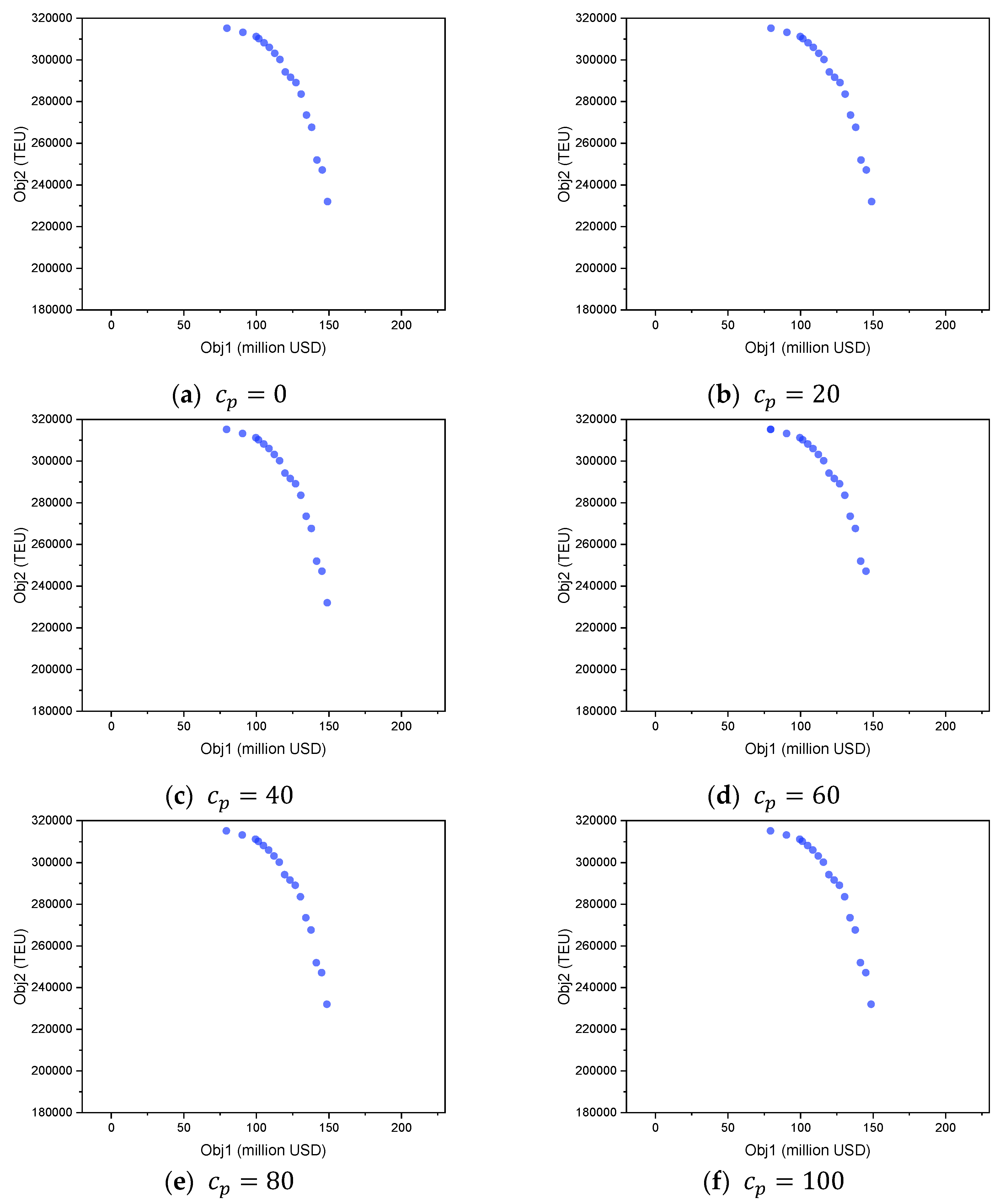
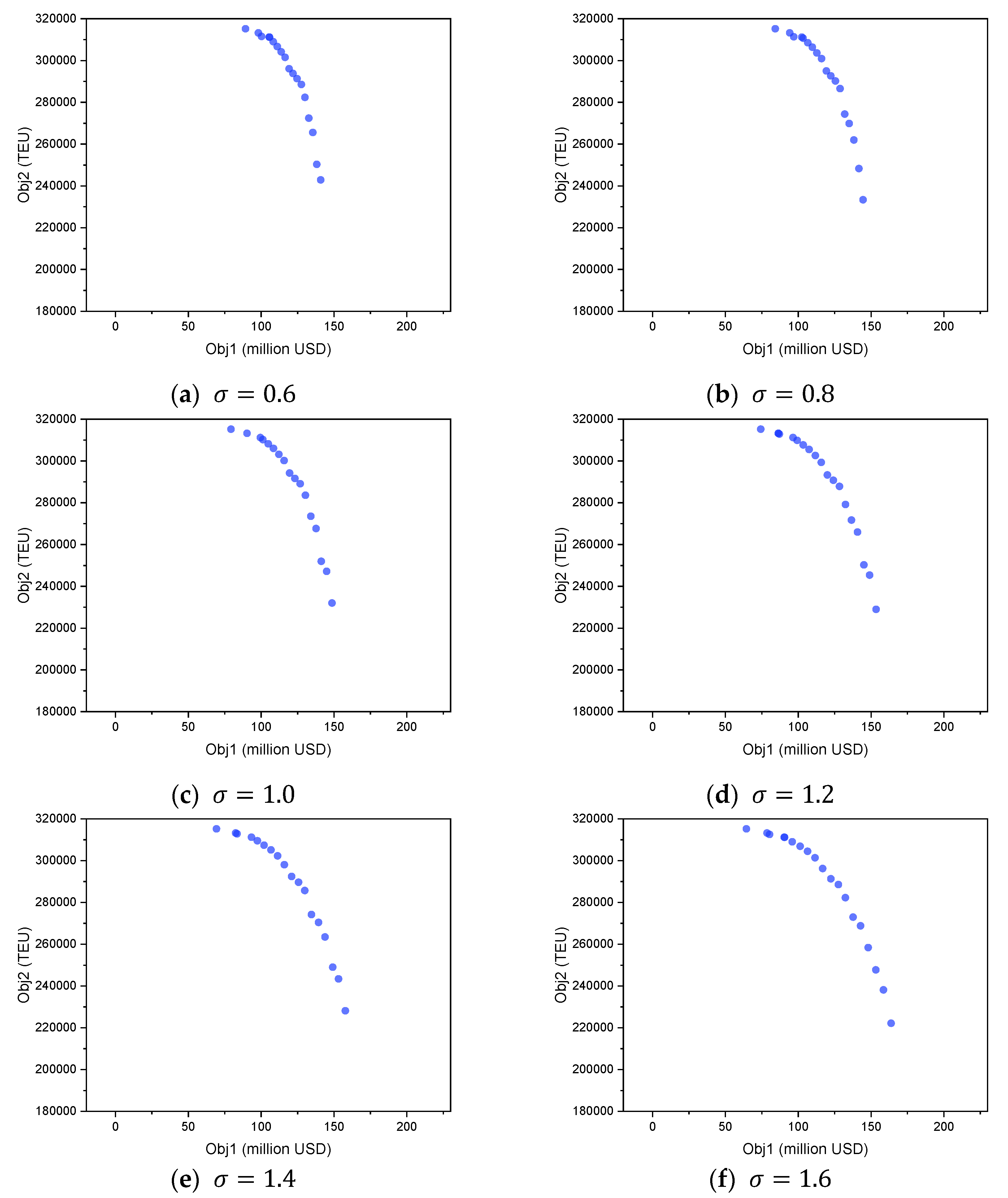
5.3.2. Sensitivity Analysis on the Surcharge Intensity

In this section, we conduct 6 experiments, aiming to illustrate the performance of our proposed model in solving instances with different surcharge intensities. We design instances by altering the unit penalty surcharge ${\mathrm{c}}_{\mathrm{p}}$ from 0 to 100 with a step size of 20 while keeping other parameters unchanged. Figure 7 shows the Pareto frontiers of all instances.

As the unit penalty surcharge ${\mathrm{c}}_{\mathrm{p}}$ increases from 0 to 100, the Pareto frontier remains largely consistent, indicating that the shipping line can maintain a similar level of performance in terms of both profit and transport volume. This stability indicates that the model is effective at finding potent mitigation strategies. The model achieves this by effectively navigating the complex trade-off between maximizing profit, increasing transport volume, and mitigating the extra penalty. It strategically reconfigures the fleet, for instance by systematically chartering out penalized China-built ships from U.S. routes and chartering in compliant ships to take their place, thereby preserving the core trade-off between Obj 1 and Obj 2.

To quantitatively dissect this mitigation strategy and reveal the underlying economic trade-offs, we analyze the total penalty paid across all Pareto-optimal solutions for each surcharge level. The results are summarized in

Table 12. Analysis of total penalty cost incurred under different surcharge intensities.

$\mathit{k}$	${\mathit{c}}_{\mathit{p}}=0$	${\mathit{c}}_{\mathit{p}}=20$	${\mathit{c}}_{\mathit{p}}=40$	${\mathit{c}}_{\mathit{p}}=60$	${\mathit{c}}_{\mathit{p}}=80$	${\mathit{c}}_{\mathit{p}}=100$
1	0	0.12	0.24	0.36	0.00	0
2	0	0.12	0.24	0.36	0.00	0
3	0	0.12	0.24	0.36	0.00	0
4	0	0.12	0.24	0.36	0.48	0
5	0	0.12	0.24	0.36	0.00	0
6	0	0.12	0.24	0.36	0.00	0
7	0	0.12	0.24	0.36	0.48	0
8	0	0.12	0.24	0.36	0.00	0
9	0	0.12	0.24	0.36	0.00	0
10	0	0.12	0.24	0.36	0.00	0
11	0	0.12	0.24	0.36	0.00	0
12	0	0.12	0.24	0.36	0.00	0
13	0	0.12	0.24	0.36	0.48	0
14	0	0.12	0.24	0.36	0.00	0
15	0	0.12	0.24	0.36	0.00	0
17	0	0.12	0.24	0.36	0.48	0
20	0	0.11	0.21	0.32	0.43	0

.

It is observed that as $c_p$ rises from 20 to 60, the total penalty incurred generally increases. This indicates that at these lower levels, it is often optimal to accept the surcharge for certain highly profitable routes where the additional cost of chartering ships to avoid using a penalized ship would exceed the penalty itself. A significant strategic shift becomes evident at $c_p=80$. At this level, some of the Pareto-optimal solutions show a total penalty of zero, indicating that for a wide range of strategies, complete avoidance has become the more profitable choice. This trend culminates at $c_p=100$, a level at which the unit penalty cost becomes so high that the total penalty across all Pareto-optimal solutions drops to zero. This illustrates the model’s sophisticated decision making, which involves calculating the most profitable strategy: paying a manageable fee on certain routes or altering fleet and route assignments to completely avoid the penalty once the cost becomes prohibitive.

5.3.3. Sensitivity Analysis on the Charter Ratio

In this section, we conduct 6 experiments, aiming to illustrate the performance of the bi-objective MIP model in solving instances with different charter ratios. The ratio is denoted as $\sigma$, where the original weekly charter-in cost and charter-out revenue for a ship of type $\mathrm{s}$ is $c_s^{\mathrm{i}\mathrm{n}}$ and $c_s^{\mathrm{o}\mathrm{u}\mathrm{t}}$, respectively. The actual charter-in cost and chareter-out revenue is ${\widehat{c}}_s^{\mathrm{i}\mathrm{n}}$ and ${\widehat{c}}_s^{\mathrm{o}\mathrm{u}\mathrm{t}}$, respectively. Then, $\sigma ={\widehat{c}}_s^{\mathrm{i}\mathrm{n}}/c_s^{\mathrm{i}\mathrm{n}}={\widehat{c}}_s^{\mathrm{o}\mathrm{u}\mathrm{t}}/c_s^{\mathrm{o}\mathrm{u}\mathrm{t}}$. To investigate the impact of varying the charter ratio of all ship types on the model’s effectiveness, we design instances by altering $\mathsf{\sigma }$ from 0.6 to 1.6 with a step size of 0.2 while keeping other parameters unchanged. Figure 8 shows the Pareto frontiers of all instances.

The sensitivity analysis on the charter ratio reveals a distinct transformation in the shape of the Pareto frontier. As the charter ratio increases, the frontier becomes progressively flatter. When the charter ratio is low (e.g., $\sigma =0.6$), the frontier is steep, meaning that achieving a higher profit requires giving up a large amount of transport volume. In contrast, when the charter ratio is high (e.g., $\sigma =1.6$), the frontier is much flatter, allowing the company to improve its profit with a smaller reduction in volume. This change is driven by the direct link between charter-in costs and charter-out revenues. In a low charter ratio environment, chartering out yields less revenue. Therefore, the company’s strategy focuses on deploying its fleet to serve a broad range of transport demands, resulting in higher transport volume. To improve profit from this state, the company must forgo large quantities of accepted demand, which explains the steep trade-off. In contrast, in a high charter ratio environment, chartering out a ship becomes a very attractive alternative. As a result, the company’s optimal strategy shifts: it serves only the demand that generates more profit than simply chartering out a ship. This reveals that a high charter ratio fundamentally changes the business priority from focusing on transport volume to strategically managing the fleet as a portfolio of assets, where chartering ships out can be a more profitable decision than using them to serve all but the most sufficiently valuable transport demands.

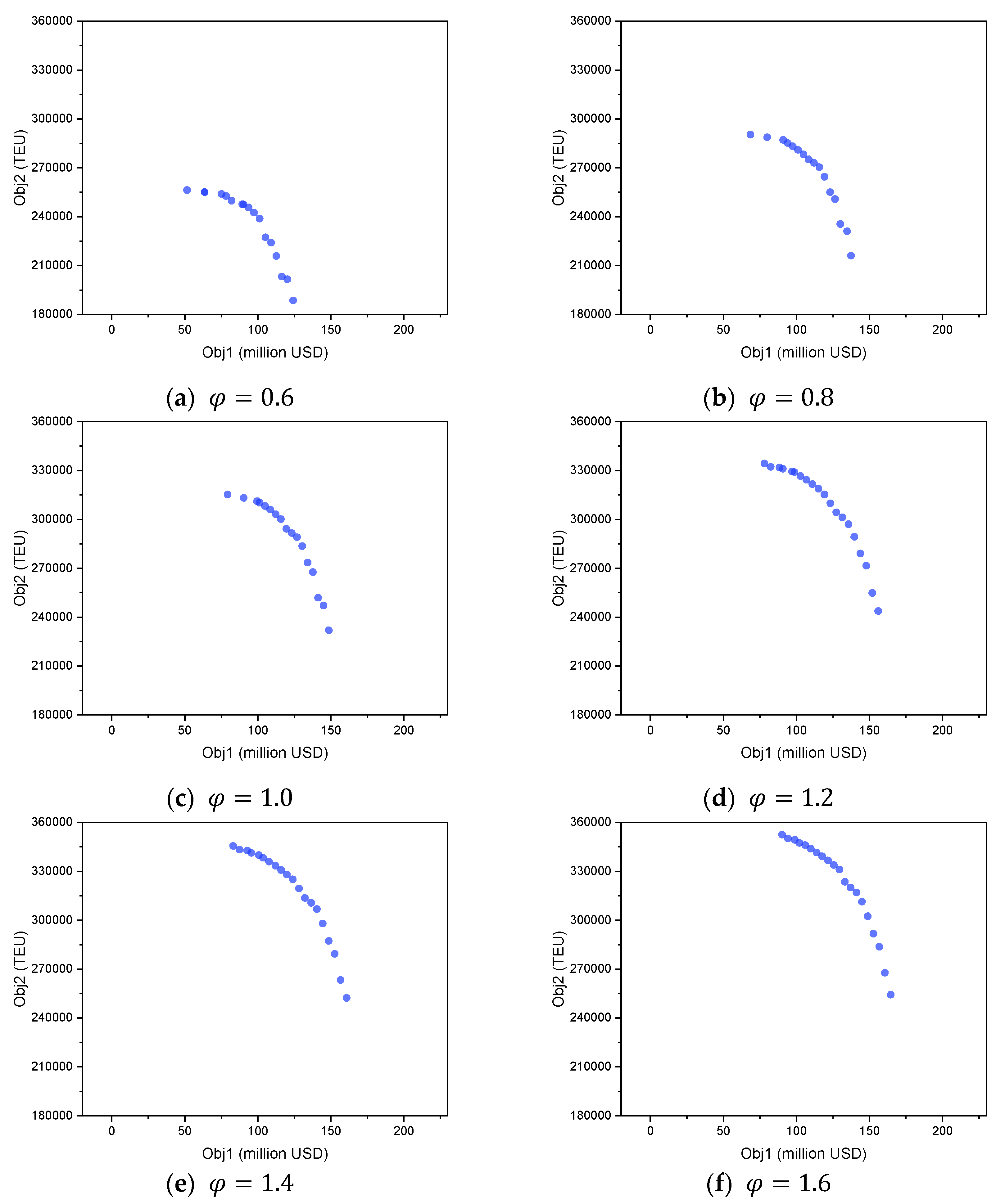
5.3.4. Sensitivity Analysis on the Transport Demand Ratio

In this section, we conduct 6 experiments, aiming to illustrate the performance of the bi-objective MIP model in solving instances with different transport demand ratios. The ratio is denoted as $\phi$, where the original weekly transport demand for an OD pair is $D_{od}$, the actual transport demand is $D_{od}^{\mathrm{a}\mathrm{c}\mathrm{t}\mathrm{u}\mathrm{a}\mathrm{l}}$, and $\phi =D_{od}^{\mathrm{a}\mathrm{c}\mathrm{t}\mathrm{u}\mathrm{a}\mathrm{l}}/D_{od}$. To investigate the impact of varying the transport demand of all OD pairs on the model’s effectiveness, we design instances by altering $\mathsf{\phi }$ from 0.6 to 1.6 with a step size of 0.2 while keeping other parameters unchanged. Figure 9 shows the Pareto frontiers of all instances.

The sensitivity analysis with respect to the transport demand ratio demonstrates the profound impact of market size on the shipping line’s operational scale and profitability. As the transport demand ratio increases from 0.6 to 1.6, representing a market shift from low to high demand, the Pareto frontier exhibits a significant and consistent outward expansion. The entire set of non-dominated solutions moves upwards and to the right, indicating that a high-demand market environment enables the simultaneous achievement of both higher total profits and greater transport volumes. At low demand levels (e.g., $\phi =0.6$), the frontier is tightly constrained, positioned close to the origin, reflecting a market where limited cargo availability severely caps the potential for both revenue and service scale. Conversely, as demand grows, the frontier expands dramatically, unlocking a much larger space of high-performance strategic options.

This outward expansion is driven by a fundamental shift in the company’s core challenge, which necessitates a corresponding shift in management strategy. In a low-demand scenario, the primary challenge of the shipping company is to find enough cargo to fill its ships, often forcing it to accept less profitable OD pairs to maintain fleet utilization. In a high-demand scenario, the market offers more cargo than the fleet can physically transport. This surplus of demand grants the shipping company a powerful strategic advantage by enabling it to prioritize more profitable OD pairs.

Given that the PRMIP model yields optimal solutions identical to those of the full MIP model (as established in Section 3.3), the detailed numerical results for the two most extreme scenarios of each of the four sensitivity analyses are presented for the PRMIP model in

Table A1. Pareto-optimal solutions of the PRMIP model ($\alpha =0.7$).

$\mathit{k}$	Obj 1 (Million USD)	Obj 2 (Million USD)	ORN	AFR (USD)	TFC (Million USD)	TBC (Million USD)	The Extra Penalty Cost	COIR (Million USD)
1	−7.56	315,250	18	643	74.44	110.79	0	−24.92
2	4.21	313,250	17	641	71.45	105.59	0	−19.52
3	7.65	311,583	17	640	70.23	104.29	0	−17.32
4	14.39	311,250	16	638	68.46	100.39	0	−15.20
5	17.83	309,583	16	637	67.24	99.09	0	−13.00
6	22.85	307,217	16	636	65.50	97.17	0	−9.84
7	27.83	304,098	16	638	63.96	95.35	0	−6.96
8	32.90	300,439	16	643	62.59	93.37	0	−4.28
9	38.18	293,564	15	655	61.83	88.37	0	−4.00
10	43.16	290,231	15	660	60.36	86.67	0	−1.36
11	48.04	285,392	15	664	58.58	84.81	0	1.96
12	53.09	274,903	14	654	55.99	76.10	0	5.28
13	58.14	271,500	14	659	54.53	74.29	0	7.92
14	63.17	264,342	14	665	52.05	72.10	0	11.60
15	68.26	252,633	14	671	48.46	68.39	0	15.52
16	73.27	243,175	13	697	48.60	64.45	0	16.88
17	78.31	231,496	13	707	44.91	61.02	0	20.56
19	83.38	215,175	12	743	42.79	56.96	0	23.36
20	88.42	189,667	11	741	35.82	48.71	0	32.32

,

Table A2. Pareto-optimal solutions of the PRMIP model ($\alpha =1.$2).

$\mathit{k}$	Obj 1 (Million USD)	Obj 2 (TEUs)	ORN	AFR (USD)	TFC (Million USD)	TBC (Million USD)	The Extra Penalty Cost	COIR (Million USD)
1	137.15	315,250	18	1102	74.44	110.79	0	−24.92
2	147.63	313,250	17	1099	71.45	105.59	0	−19.52
3	149.64	311,917	17	1098	70.47	104.55	0	−17.76
4	156.14	311,250	16	1093	68.46	100.39	0	−15.20
5	159.07	309,398	16	1093	67.22	99.08	0	−12.92
6	162.10	307,398	16	1092	65.75	97.52	0	−10.28
7	165.35	305,175	16	1092	64.28	95.93	0	−7.64
8	168.34	302,648	16	1098	63.45	94.65	0	−6.00
9	171.37	300,050	16	1104	62.40	93.36	0	−4.00
10	174.58	294,231	15	1124	62.32	88.89	0	−4.88
11	177.79	291,898	15	1127	61.10	87.52	0	−2.68
12	180.72	289,675	15	1133	60.12	86.39	0	−0.92
13	183.90	285,350	15	1145	58.89	85.05	0	1.14
15	186.89	273,355	14	1158	56.42	78.17	0	5.00
16	190.00	267,581	14	1176	55.20	76.80	0	7.20
19	193.11	251,858	13	1233	53.77	73.20	0	9.44
20	196.39	243,300	13	1216	49.85	65.10	0	15.60

,

Table A3. Pareto-optimal solutions of the PRMIP model ($c_p=0$).

$\mathit{k}$	Obj 1 (Million USD)	Obj 2 (Million USD)	ORN	AFR (USD)	TFC (Million USD)	TBC (Million USD)	The Extra Penalty Cost	COIR (Million USD)
1	149.06	232,016	13	1014	45.57	61.42	0.00	20.56
2	145.44	247,188	13	997	50.34	65.90	0.00	15.20
3	141.76	251,997	13	1027	53.77	73.20	0.00	9.92
4	138.12	267,675	14	951	53.52	73.30	0.00	10.24
5	134.54	273,564	14	963	56.42	78.17	0.00	5.48
6	130.84	283,641	15	957	58.6	84.61	0.00	2.36
7	127.28	289,119	15	945	59.87	86.10	0.00	0.00
8	123.61	291,675	15	940	61.10	87.50	0.00	−2.20
9	119.95	294,230	15	936	62.32	88.89	0.00	−4.40
10	116.26	300,208	16	917	62.40	93.33	0.00	−3.52
11	112.64	303,203	16	914	63.69	94.94	0.00	−5.96
12	108.95	306,064	16	909	64.77	96.48	0.00	−8.04
13	105.32	308,216	16	909	66.24	97.95	0.00	−10.68
14	101.66	310,250	16	910	67.73	99.61	0.00	−13.40
15	99.92	311,250	16	910	68.46	100.39	0.00	−14.72
17	90.74	313,250	17	915	71.45	105.59	0.00	−19.04
20	79.74	315,250	18	918	74.44	110.79	0.00	−24.44

,

Table A4. Pareto-optimal solutions of the PRMIP model ($c_p=100$).

$\mathit{k}$	Obj 1 (Million USD)	Obj 2 (TEUs)	ORN	AFR (USD)	TFC (Million USD)	TBC (Million USD)	The Extra Penalty Cost	COIR (Million USD)
1	148.58	232,016	13	1014	45.57	61.42	0	20.08
2	144.96	247,188	13	997	50.34	65.9	0	14.72
3	141.28	251,997	13	1027	53.77	73.2	0	9.44
4	137.64	267,675	14	951	53.52	73.3	0	9.76
5	134.06	273,564	14	963	56.42	78.17	0	5.00
6	130.36	283,641	15	957	58.6	84.61	0	1.88
7	126.80	289,119	15	945	59.87	86.1	0	−0.48
8	123.13	291,675	15	940	61.1	87.5	0	−2.68
9	119.47	294,230	15	936	62.32	88.89	0	−4.88
10	115.74	300,230	16	919	62.59	93.33	0	−4.28
11	112.16	303,203	16	914	63.69	94.94	0	−6.44
12	108.47	306,064	16	909	64.77	96.48	0	−8.52
13	104.84	308,216	16	909	66.24	97.95	0	−11.16
14	101.18	310,250	16	910	67.73	99.61	0	−13.88
15	99.44	311,250	16	910	68.46	100.39	0	−15.20
17	90.26	313,250	17	915	71.45	105.59	0	−19.52
20	79.26	315,250	18	918	74.44	110.79	0	−24.92

,

Table A5. Pareto-optimal solutions of the PRMIP model ($\sigma =0.6$).

$\mathit{k}$	Obj 1 (Million USD)	Obj 2 (Million USD)	ORN	AFR (USD)	TFC (Million USD)	TBC (Million USD)	The Extra Penalty Cost	COIR (Million USD)
1	140.88	242,871	13	1014	49.82	65.04	0	9.41
2	138.16	250,335	13	1036	53.77	73.2	0	5.66
3	135.44	265,583	14	990	55.2	76.8	0	4.32
4	132.72	272,440	14	967	56.17	78	0	3.26
5	130.02	282,391	15	960	58.36	84.31	0	1.31
6	127.59	288,564	15	946	59.63	85.82	0	−0.02
7	124.61	291,342	15	940	60.85	87.24	0	−1.34
8	121.86	293,827	15	936	62.08	88.52	0	−2.66
9	119.14	296,108	16	927	61.61	92.32	0	−1.60
10	116.44	301,536	16	917	62.96	94.09	0	−3.16
11	113.77	304,175	16	913	64.04	95.6	0	−4.40
12	111.07	306,730	16	909	65.26	97	0	−5.64
13	108.26	309,064	16	910	66.97	98.82	0	−7.49
14	105.69	311,216	16	910	68.44	100.29	0	−9.07
15	105.52	311,250	16	910	68.46	100.39	0	−9.12
16	100.25	311,550	17	914	70.2	104.19	0	−10.34
17	98.07	313,250	17	915	71.45	105.59	0	−11.71
20	89.23	315,250	18	918	74.44	110.79	0	−14.95

,

Table A6. Pareto-optimal solutions of the PRMIP model ($\sigma =1.6$).

$\mathit{k}$	Obj 1 (Million USD)	Obj 2 (Million USD)	ORN	AFR (USD)	TFC (Million USD)	TBC (Million USD)	The Extra Penalty Cost	COIR (Million USD)
1	163.76	222,188	12	1062	45.73	59.3	0.72	33.54
2	158.53	238,175	13	1011	47.62	63.25	0.72	29.31
3	153.30	247,744	13	997	50.58	66.1	0.72	23.62
4	148.04	258,411	14	958	50.51	70.37	0.72	22.02
5	142.81	268,855	14	945	53.52	73.46	0.72	16.38
6	137.64	273,008	14	963	56.17	77.97	0.72	9.47
7	132.38	282,325	15	960	58.33	84.23	0.72	4.61
8	127.59	288,564	15	946	59.63	85.82	0.72	0.70
9	122.41	291,342	15	940	60.85	87.24	0.72	−2.82
10	116.76	296,275	16	922	61.32	92.12	0.18	−2.88
11	111.52	301,411	16	917	62.93	94.04	0.72	−7.30
12	106.38	304,494	16	910	64.01	95.6	0.72	−10.62
13	101.31	306,916	16	908	65.28	97.01	0.72	−14.40
14	95.83	309,064	16	910	66.97	98.82	0.72	−19.20
15	90.62	311,216	16	910	68.44	100.29	0.72	−23.42
16	90.37	311,250	16	910	68.46	100.39	0.72	−23.55
17	80.28	312,583	17	915	70.96	105.07	0.72	−29.06
18	78.60	313,250	17	915	71.45	105.59	0.72	−30.46
20	64.44	315,250	18	918	74.44	110.79	0.64	−39.10

,

Table A7. Pareto-optimal solutions of the PRMIP model ($\phi =0.6$).

$\mathit{k}$	Obj 1 (Million USD)	Obj 2 (Million USD)	ORN	AFR (USD)	TFC (Million USD)	TBC (Million USD)	The Extra Penalty Cost	COIR (Million USD)
1	124.10	188,653	12	1069	43.62	57.08	0	23.08
2	120.25	201,673	13	1016	45	60.48	0	20.76
3	116.41	203,291	13	1062	47.72	67.72	0	15.84
4	112.59	215,907	13	980	47.91	67.98	0	16.88
5	108.99	224,070	14	994	51.57	73.47	0	11.16
6	105.21	227,403	14	996	54.02	76.08	0	8.76
7	101.22	238,847	15	961	54.29	80.65	0	6.60
8	97.41	242,514	15	952	56	82.61	0	4.92
9	93.62	245,736	15	953	58.21	84.98	0	2.56
10	90.08	247,536	15	954	59.65	86.42	0	−0.12
11	89.39	247,670	15	954	59.87	86.55	0	−0.60
12	82.06	249,794	16	935	59.65	90.73	0	−1.32
13	78.24	252,683	16	936	61.61	92.84	0	−3.84
14	75.15	253,970	16	937	62.81	93.95	0	−6.08
17	63.56	255,170	17	940	65.79	99.15	0	−11.48
19	63.58	255,150	17	940	65.77	99.09	0	−11.52
20	51.52	256,370	18	942	68.78	104.35	0	−16.88

and

Table A8. Pareto-optimal solutions of the PRMIP model ($\phi =1.6$).

$\mathit{k}$	Obj 1 (Million USD)	Obj 2 (Million USD)	ORN	AFR (USD)	TFC (Million USD)	TBC (Million USD)	The Extra Penalty Cost	COIR (Million USD)
1	164.54	254,346	13	1035	50.14	63.88	0	15.12
2	160.51	267,788	13	1018	52.88	70.07	0	10.64
3	156.71	283,746	14	977	54.58	73.91	0	7.88
4	152.70	291,746	14	981	58.22	76.82	0	1.36
5	148.75	302,493	15	979	60.51	85.65	0	−1.50
6	144.87	311,437	15	971	63.11	88.41	0	−6.24
7	141.09	317,048	15	966	65.06	90.36	0	−9.76
8	137.03	320,048	15	959	66.29	91.8	0	−11.96
9	133.11	323,604	16	948	66.41	96.33	0	−11.24
10	129.39	331,160	16	934	67.78	98.36	0	−13.92
11	125.53	333,937	16	929	69.01	99.78	0	−16.12
12	121.58	336,715	16	924	70.23	101.23	0	−18.32
13	117.55	339,271	16	920	71.45	102.76	0	−20.52
14	113.81	341,604	16	917	72.68	104.23	0	−22.72
15	109.77	343,937	16	918	74.39	106.05	0	−25.80
16	106.01	346,160	16	918	75.86	107.66	0	−28.44
17	102.00	347,471	17	925	77.62	111.51	0	−30.56
18	98.83	349,360	17	925	78.84	112.86	0	−32.76
19	94.15	350,226	18	927	80.12	116.24	0	−34.36
20	90.10	352,560	18	928	81.83	118.06	0	−37.44

in Appendix B.

6. Conclusions

Container liner shipping companies operate within a complex environment where they must balance profitability and service reliability, all while navigating evolving regulatory policies such as surcharges imposed on China-built ships calling at U.S. ports. These challenges complicate strategic planning related to route deployment, ship assignment, and demand acceptance, requiring integrated decision-making frameworks.

To address these challenges, this study develops a bi-objective MIP model for the HSR-DA problem. We establish a series of theorems to analyze the mathematical structure of the model. Specifically, we prove that the route operation decision variables and ship assignment variables must remain integers due to the practical infeasibility of fractional route operation and ship assignment, while the chartering constraints form a TU matrix, which allows the corresponding variables to be relaxed to continuous values without loss of integrality. Additionally, we demonstrate that the Pareto frontier consists of a finite union of line segments. Within each segment, it is continuous and piecewise linear, while generally being non-convex and exhibiting discontinuities. Based on these theorems, we reformulate the original MIP into a PRMIP model. We demonstrate that the PRMIP model can generate the same optimal objective value as the one obtained by the MIP model when solving the same instance, while significantly improving computational efficiency. Furthermore, we can always find an optimal solution to the PRMIP model such that it is equivalent to an optimal solution to the MIP model. These theoretical insights provide a solid foundation for enhancing solution efficiency and understanding the structural characteristics of the Pareto frontier.

Computational experiments conducted with real-world-inspired scenarios highlight the practical effectiveness of the proposed model. The results demonstrate a clear trade-off between maximizing profitability and maximizing transport volumes, represented through an explicitly characterized Pareto frontier. Notably, the model consistently avoids costly surcharges for China-built ships through strategic fleet assignment and chartering decisions, underscoring its ability to inform operational strategies under complex regulatory constraints. In scenarios prioritizing profit maximization, the accepted transport volume decreases while the average freight rate increases, confirming the necessity of targeted and strategic route selection and demand acceptance. Sensitivity analysis further reveals that variations in freight rates significantly affect the structure of optimal decisions. Higher freight rates provide greater flexibility, allowing operators to selectively expand transport volumes while enhancing profitability simultaneously. Conversely, lower freight rates necessitate stringent selectivity in demand acceptance, reinforcing the importance of adaptive decision making in response to market fluctuations.

Future work can extend our model by addressing several key areas to enhance its robustness and practical applicability:

• Incorporating transshipment and empty container repositioning: The current model excludes transshipment and empty container repositioning, which are critical for operational efficiency. Future work can optimize cargo routing and empty container flows, potentially using foldable containers or leasing strategies to reduce costs and improve container utilization [77,78,79].
• Incorporating variable sailing speeds: Allowing speed to be a decision variable can build a more comprehensive framework. This extension can capture the critical trade-off between fuel costs and service efficiency by directly linking sailing speed to operational fuel expenses and strategic ship allocation. Higher speeds increase fuel consumption, while lower speeds extend voyage times, which may require additional ships to maintain fixed service frequencies. Recent studies provide valuable insights in this field. For example, a holistic optimization model was developed [10] that integrates sailing speed optimization with port service frequency, fleet deployment, and ship schedule design, demonstrating the benefits of joint tactical planning. Similarly, a multi-objective mixed-integer linear programming model was proposed [27] to optimize sailing speed, as well as fleet deployment and routing under carbon tax regulations, achieving cost savings of up to 15% and emission reductions of 20% on a transatlantic route. A hybrid dynamic model with receding horizon speed optimization was introduced [80], emphasizing schedule reliability and energy efficiency when port handling times are uncertain. In addition, the focus was on sailing speed optimization for near-sea shipping services, integrating container routes to improve operational efficiency [81]. With these advancements, future work can co-optimize shipping networks, fleet deployment, and sailing speeds, providing in-depth insights into how shipping companies can balance strategic and operational strategies while adapting to external policies to maintain economic and environmental sustainability.
• The challenge of expanding models to accommodate multinational regulatory compliance and carbon pricing mechanisms: The current fleet deployment model can be extended to incorporate either multinational regulatory compliance or carbon pricing mechanisms to enhance its applicability in a globalized market. Dynamic fleet reallocation can further support these extensions by enabling real-time adjustments to ship assignments in response to varying regulatory requirements or carbon pricing impacts [82]. Multi-objective optimization models have been proposed to incorporate the EU Emissions Trading System (EU ETS) into China–Europe liner shipping, optimizing speed to balance emissions and costs [83]. Frameworks for carbon and cost accounting under EU ETS focus on operational adjustments like fuel choice and speed optimization to ensure compliance [84]. Bi-level programming models incorporate carbon taxes into network design, addressing route planning and fleet deployment under environmental constraints [85]. Compliance with diverse international standards, such as those for sustainable maritime operations, has also been explored to ensure operational feasibility across jurisdictions [86]. Future work could extend the current fleet deployment model to incorporate either compliance with multinational regulations, such as EU ETS and other global standards, or carbon pricing mechanisms into strategies like speed optimization, fuel choice, and route planning. These models could explore collaborative agreements or standardized practices to address regulatory variations across jurisdictions, ensuring cost-effective compliance and sustainability in a globalized market.

References

1. Christiansen, M.; Fagerholt, K.; Nygreen, B.; Ronen, D. Optimization in liner shipping. 4OR A Q. J. Oper. Res. 2017, 15, 327–341. [Google Scholar]
2. Notice of Action and Proposed Action in Section 301 Investigation of China’s Targeting the Maritime, Logistics, and Shipbuilding Sectors for Dominance, Request for Comments. Available online: https://www.federalregister.gov/documents/2025/04/23/2025-06927/notice-of-action-and-proposed-action-in-section-301-investigation-of-chinas-targeting-the-maritime (accessed on 5 May 2025).
3. U.S. Proposes Port Fees on Chinese-Built Ships and Operators to Counter China’s Shipping Dominance. Available online: https://www.hklaw.com/en/insights/publications/2025/03/us-proposes-port-fees-on-chinese-built-ships (accessed on 5 May 2025).
4. U.S. Revises Section 301 Tariffs on Chinese Vessels Amid Industry Pushback. Available online: https://www.shipuniverse.com/news/u-s-revises-section-301-tariffs-on-chinese-vessels-amid-industry-pushback/ (accessed on 5 May 2025).
5. USTR Section 301 Action on China’s Targeting of the Maritime, Logistics, and Shipbuilding Sectors for Dominance. Available online: https://ustr.gov/about/policy-offices/press-office/press-releases/2025/april/ustr-section-301-action-chinas-targeting-maritime-logistics-and-shipbuilding-sectors-dominance (accessed on 16 July 2025).
6. Proposed U.S. Port Fees on China-Built Ships Begins Choking Coal, Agriculture Exports. Available online: https://www.reuters.com/world/us/proposed-us-port-fees-china-built-ships-begins-choking-coal-agriculture-exports-2025-03-19/ (accessed on 16 July 2025).
7. Trump Is Targeting China-Made Containerships in New Flank of Global Economic War on the Oceans. Available online: https://www.cnbc.com/2025/03/11/trump-pursues-new-trade-war-on-seas-targeting-china-containerships.html (accessed on 16 July 2025).
8. Launch of the Review of Maritime Transport 2024. Available online: https://unctad.org/meeting/launch-review-maritime-transport-2024 (accessed on 5 May 2025).
9. Wang, Y.; Zhang, H.; Wang, T.; Liu, J. Heterogeneous vessel fleet co-management for liner alliances under profit-sharing agreement and weekly-dependent demand. Transp. Res. Part E Logist. Transp. Rev. 2024, 188, 103494. [Google Scholar] [CrossRef]
10. Pasha, J.; Dulebenets, M.A.; Kavoosi, M.; Abioye, O.F.; Theophilus, O.; Wang, H.; Kampmann, R.; Guo, W. Holistic tactical-level planning in liner shipping: An exact optimization approach. J. Shipp. Trade 2020, 5, 8. [Google Scholar] [CrossRef]
11. Meng, L.; Ge, H.; Wang, X.; Yan, W.; Han, C. Optimization of ship routing and allocation in a container transport network considering port congestion: A variational inequality model. Ocean Coast. Manag. 2023, 244, 106798. [Google Scholar] [CrossRef]
12. Ting, S.C.; Tzeng, G.H. Ship scheduling and cost analysis for route planning in liner shipping. Marit. Econ. Logist. 2003, 5, 378–392. [Google Scholar] [CrossRef]
13. Cariou, P.; Cheaitou, A.; Larbi, R.; Hamdan, S. Liner shipping network design with emission control areas: A genetic algorithm-based approach. Transp. Res. Part D Transp. Environ. 2018, 63, 604–621. [Google Scholar] [CrossRef]
14. Fagerholt, K.; Gausel, O.B.; Rakke, J.G.; Psaraftis, H.N. Maritime routing and speed optimization with emission control areas. Transp. Res. Part C Emerg. Technol. 2015, 55, 419–430. [Google Scholar] [CrossRef]
15. Wen, M.; Ropke, S.; Petersen, H.L.; Larsen, R.; Madsen, O.B. Full-shipload tramp ship routing and scheduling with variable speeds. Comput. Oper. Res. 2016, 70, 1–8. [Google Scholar] [CrossRef]
16. Mahmoodjanloo, M.; Chen, G.; Asian, S.; Iranmanesh, S.H.; Tavakkoli-Moghaddam, R. In-port multi-ship routing and scheduling problem with draft limits. Marit. Policy Manag. 2021, 48, 966–987. [Google Scholar] [CrossRef]
17. Venturini, G.; Iris, Ç.; Kontovas, C.A.; Larsen, A. The multi-port berth allocation problem with speed optimization and emission considerations. Transp. Res. Part D Transp. Environ. 2017, 54, 142–159. [Google Scholar] [CrossRef]
18. Song, D.P.; Li, D.; Drake, P. Multi-objective optimization for a liner shipping service from different perspectives. Transp. Res. Procedia 2017, 25, 1441–1452. [Google Scholar] [CrossRef]
19. Xiao, P.; Wang, H. Ship type selection and cost optimization of marine container ships based on genetic algorithm. Appl. Sci. 2024, 14, 9816. [Google Scholar] [CrossRef]
20. Liu, T.; Liu, J.; Xu, H. A multi-population multi-objective maritime inventory routing optimization algorithm with three-level dynamic encoding. Sci. Rep. 2025, 15, 5701. [Google Scholar] [CrossRef] [PubMed]
21. Wang, S.; Meng, Q.; Lee, C.Y. Liner container assignment model with transit-time-sensitive container shipment demand and its applications. Transp. Res. Part B Methodol. 2016, 85, 97–119. [Google Scholar] [CrossRef]
22. Wang, T.; Liu, J.; Wang, Y.; Jin, Y.; Wang, S. Dynamic flexible allocation of slots in container line transport. Sustainability 2024, 16, 9146. [Google Scholar] [CrossRef]
23. Park, S.; Kim, H.; Lee, S. Regulatory compliance and operational efficiency in maritime transport: Strategies and insights. Transp. Policy 2024, 146, 130–140. [Google Scholar] [CrossRef]
24. Tran, N.K.; Haasis, H.D. Literature survey of network optimization in container liner shipping. Flex. Serv. Manuf. J. 2015, 27, 139–179. [Google Scholar] [CrossRef]
25. Gu, Y.; Wang, Y.; Zhang, J. Fleet deployment and speed optimization of container ships considering bunker fuel consumption heterogeneity. Manag. Syst. Eng. 2022, 1, 3. [Google Scholar] [CrossRef]
26. Jiang, X.; Mao, H.; Zhang, H. Simultaneous optimization of the liner shipping route and ship schedule designs with time windows. Math. Probl. Eng. 2020, 2020, 3287973. [Google Scholar] [CrossRef]
27. Pasha, J.; Dulebenets, M.A.; Fathollahi-Fard, A.M.; Tian, G.; Lau, Y.Y.; Singh, P.; Liang, B. An integrated optimization method for tactical-level planning in liner shipping with heterogeneous ship fleet and environmental considerations. Adv. Eng. Inform. 2021, 48, 101299. [Google Scholar] [CrossRef]
28. Zhao, Y.; Peng, Z.; Zhou, J.; Notteboom, T.; Ma, Y. Toward green container liner shipping: Joint optimization of heterogeneous fleet deployment, speed optimization, and fuel bunkering. Int. Trans. Oper. Res. 2024, 32, 863–887. [Google Scholar] [CrossRef]
29. Brouer, B.D.; Desaulniers, G.; Pisinger, D. A matheuristic for the liner shipping network design problem. Transp. Res. Part E Logist. Transp. Rev. 2014, 72, 42–59. [Google Scholar] [CrossRef]
30. Cheaitou, A.; Hamdan, S.; Larbi, R. Liner shipping network design with sensitive demand. Marit. Bus. Rev. 2021, 6, 293–313. [Google Scholar] [CrossRef]
31. Xia, J.; Li, K.X.; Ma, H.; Xu, Z. Joint planning of fleet deployment, speed optimization, and cargo allocation for liner shipping. Transp. Sci. 2015, 49, 922–938. [Google Scholar] [CrossRef]
32. Lai, X.; Wu, L.; Wang, K.; Wang, F. Robust ship fleet deployment with shipping revenue management. Transp. Res. Part B Methodol. 2022, 161, 169–196. [Google Scholar] [CrossRef]
33. Zhao, Z.; Wang, X.; Wang, H.; Cheng, S.; Liu, W. Fleet deployment optimization for LNG shipping vessels considering the influence of mixed factors. J. Mar. Sci. Eng. 2022, 10, 2034. [Google Scholar] [CrossRef]
34. Psaraftis, H.N.; Kontovas, C.A. Speed models for energy-efficient maritime transportation: A taxonomy and survey. Transp. Res. Part C Emerg. Technol. 2013, 26, 331–351. [Google Scholar] [CrossRef]
35. Bertho, F.; Borchert, I.; Mattoo, A. The trade-reducing effects of restrictions on liner shipping. J. Comp. Econ. 2016, 44, 231–242. [Google Scholar] [CrossRef]
36. Notteboom, T.; Pallis, T.; Rodrigue, J.P. Disruptions and resilience in global container shipping and ports: The COVID-19 pandemic versus the 2008–2009 financial crisis. Marit. Econ. Logist. 2021, 23, 179. [Google Scholar] [CrossRef]
37. Bichou, K. Port Operations, Planning and Logistics, 1st ed.; CRC Press: Boca Raton, FL, USA, 2014. [Google Scholar]
38. Jin, L.; Chen, J.; Chen, Z.; Sun, X.; Yu, B. Impact of COVID-19 on China’s international liner shipping network based on AIS data. Transp. Policy 2022, 121, 90–99. [Google Scholar] [CrossRef]
39. Ksciuk, J.; Kuhlemann, S.; Tierney, K.; Koberstein, A. Uncertainty in maritime ship routing and scheduling: A Literature review. Eur. J. Oper. Res. 2023, 308, 499–524. [Google Scholar] [CrossRef]
40. Zhu, Z.; Zhang, S.; Cao, Z. Exact and heuristic methods for the integrated optimisation of vessel deployment and liner shipping routing schedule. Int. J. Syst. Sci. Oper. Logist. 2025, 12, 2505920. [Google Scholar] [CrossRef]
41. Verschuur, J.; Koks, E.E.; Hall, J.W. Port disruptions due to natural disasters: Insights into port and logistics resilience. Transp. Res. Part D Transp. Environ. 2020, 85, 102393. [Google Scholar] [CrossRef]
42. Elmi, Z.; Singh, P.; Meriga, V.K.; Goniewicz, K.; Borowska-Stefańska, M.; Wiśniewski, S.; Dulebenets, M.A. Uncertainties in liner shipping and ship schedule recovery: A state-of-the-art review. J. Mar. Sci. Eng. 2022, 10, 563. [Google Scholar] [CrossRef]
43. Zheng, H.; Negenborn, R.R.; Lodewijks, G. Robust distributed predictive control of waterborne AGVs—A cooperative and cost-effective approach. IEEE Trans. Cybern. 2017, 48, 2449–2461. [Google Scholar] [CrossRef] [PubMed]
44. Han, S.W.; Lee, E.H.; Kim, D.K. Multi-objective optimization for skip-stop strategy based on smartcard data considering total travel time and equity. Transp. Res. Rec. 2021, 2675, 841–852. [Google Scholar] [CrossRef]
45. Rajabighamchi, F.; Hajlou, E.M.H.; Hassannayebi, E. A multi-objective optimization model for robust skip-stop scheduling with earliness and tardiness penalties. Urban Rail Transit 2019, 5, 172–185. [Google Scholar] [CrossRef]
46. Shang, P.; Li, R.; Liu, Z.; Yang, L.; Wang, Y. Equity-oriented skip-stopping schedule optimization in an oversaturated urban rail transit network. Transp. Res. Part C Emerg. Technol. 2018, 89, 321–343. [Google Scholar] [CrossRef]
47. Lee, E.H.; Jeong, J. Accessible taxi routing strategy based on travel behavior of people with disabilities incorporating vehicle routing problem and Gaussian mixture model. Travel Behav. Soc. 2024, 34, 100687. [Google Scholar] [CrossRef]
48. Lee, E.H.; Kim, G.J. Multi-objective optimization of submerged floating tunnel route considering structural safety and total travel time. Struct. Eng. Mech. Int. J. 2023, 88, 323–334. [Google Scholar]
49. Wen, X.; Chen, Q.; Yin, Y.Q.; Lau, Y.Y.; Dulebenets, M.A. Multi-objective optimization for ship scheduling with port congestion and environmental considerations. J. Mar. Sci. Eng. 2024, 12, 114. [Google Scholar] [CrossRef]
50. Revised US Port Fee Plan Leaves Important Questions Unanswered, Lawyers Argue. Available online: https://www.lloydslist.com/LL1153244/Revised-US-port-fee-plan-leaves-important-questions-unanswered-lawyers-argue (accessed on 5 May 2025).
51. Hoffman, A.J.; Kruskal, J.B. Integral boundary points of convex polyhedra. In 50 Years of Integer Programming 1958–2008: From the Early Years to the State-of-the-Art; Springer: Berlin/Heidelberg, Germany, 2010; pp. 49–76. [Google Scholar]
52. Mavrotas, G. Effective implementation of the ε-constraint method in multi-objective mathematical programming problems. Appl. Math. Comput. 2009, 213, 455–465. [Google Scholar] [CrossRef]
53. Zhao, W.; Wang, Y.; Zhang, Z.; Wang, H. Multicriteria ship route planning method based on improved particle swarm optimization–genetic algorithm. J. Mar. Sci. Eng. 2021, 9, 357. [Google Scholar] [CrossRef]
54. Chen, Y.; Li, J.; Hao, X.; Zhao, Y.; Gong, Y. Dispatch optimization of maritime rescue forces in Arctic shipping based on the comparison of TOPSIS and the weighted scoring method. In Proceedings of the ISOPE International Ocean and Polar Engineering Conference, Sapporo, Japan, 19–24 June 2022; p. ISOPE-I. [Google Scholar]
55. Farmakis, P.; Chassiakos, A.; Karatzas, S. A Multi-Objective Tri-Level Algorithm for Hub-and-Spoke Network in Short Sea Shipping Transportation. Algorithms 2023, 16, 379. [Google Scholar] [CrossRef]
56. Das, I.; Dennis, J.E. A closer look at drawbacks of minimizing weighted sums of objectives for Pareto set generation in multicriteria optimization problems. Struct. Optim. 1997, 14, 63–69. [Google Scholar] [CrossRef]
57. Deb, K.; Sindhya, K.; Hakanen, J. Multi-objective optimization. In Decision Sciences, 1st ed.; Ravindran, A.R., Ed.; CRC Press: Boca Raton, FL, USA, 2016; pp. 161–200. [Google Scholar]
58. CMA CGM, Maersk, and COSCO Compete for the Market Lead in the Asia–North America Trade. Available online: https://globalmaritimehub.com/cma-cgm-maersk-and-cosco-compete-for-the-market-lead-in-the-asia-north-america-trade.html (accessed on 5 May 2025).
59. Better Ways, Making Supply Chains More Sustainable Every Day. Available online: https://www.cma-cgm.com/about/the-group (accessed on 5 May 2025).
60. Evolution of Vessel Size on the Asia-Europe Route. Available online: https://www.porttechnology.org/news/evolution-of-vessel-size-on-the-asia-europe-route/ (accessed on 5 May 2025).
61. Alphaliner Top 100. Available online: https://alphaliner.axsmarine.com/PublicTop100/ (accessed on 5 May 2025).
62. Most Shipping Lines Can Avoid US Port Fees but Cosco Faces Major Challenge. Available online: https://www.lloydslist.com/LL1153279/Most-shipping-lines-can-avoid-US-port-fees-but-Cosco-faces-major-challenge (accessed on 5 May 2025).
63. Ocean Alliance Day9 Route Products. Available online: https://www.cargoespi.com/blogs/news/ocean-alliance-day9-routes (accessed on 5 May 2025).
64. MSC China-North Europe Sea Route. Available online: https://www.shiphub.co/msc-china-north-europe-sea-route/ (accessed on 5 May 2025).
65. The Future Standalone MSC East/West Network. Available online: https://www.msc.com/en/solutions/our-trade-services/east-west-network (accessed on 5 May 2025).
66. Maersk and MSC Switch to Liverpool Port Permanently. Available online: https://www.logisticsmanager.com/maersk-and-msc-switch-to-liverpool-port-permanently/ (accessed on 5 May 2025).
67. MSC Revises Its Asia to North America West Coast Network. Available online: https://www.msc.com/en/newsroom/customer-advisories/2025/february/msc-revises-its-asia-to-north-america-west-coast-network (accessed on 5 May 2025).
68. THE Alliance Announces Updated Service Network for 2024. Available online: https://container-news.com/the-alliance-announces-updated-service-network-for-2024/ (accessed on 5 May 2025).
69. Containerized Cargo Flows on Major Container Trade Routes in 2024, by Trade Route. Available online: https://www.statista.com/statistics/253988/estimated-containerized-cargo-flows-on-major-container-trade-routes/ (accessed on 5 May 2025).
70. Review of Maritime Transport 2024. Available online: https://unctad.org/publication/review-maritime-transport-2024 (accessed on 5 May 2025).
71. Drewry World Container Index. Available online: https://www.drewry.co.uk/supply-chain-advisors/supply-chain-expertise/world-container-index-assessed-by-drewry (accessed on 5 May 2025).
72. Freightos Container Shipping Cost Calculator. Available online: https://www.freightos.com/freight-resources/container-shipping-cost-calculator-free-tool/ (accessed on 5 May 2025).
73. Drewry Intra-Asia Container Index. Available online: https://www.drewry.co.uk/supply-chain-advisors/supply-chain-expertise/intra-asia-container-index (accessed on 5 May 2025).
74. Wang, S.; Meng, Q. Sailing speed optimization for container ships in a liner shipping network. Transp. Res. Part E Logist. Transp. Rev. 2012, 48, 701–714. [Google Scholar] [CrossRef]
75. Ship & Bunker. Global 20 Ports Average Bunker Prices. Available online: https://shipandbunker.com/prices/av/global/av-g20-global-20-ports-average (accessed on 5 May 2025).
76. Wilkinson, L. Revising the Pareto Chart. Am. Stat. 2006, 60, 332–334. [Google Scholar] [CrossRef]
77. Wang, S.; Meng, Q. Liner ship fleet deployment with container transshipment operations. Transp. Res. Part E Logist. Transp. Rev. 2012, 48, 470–484. [Google Scholar] [CrossRef]
78. Liu, M.; Liu, Z.; Liu, R.; Sun, L. Distribution-free approaches for an integrated cargo routing and empty container repositioning problem with repacking operations in liner shipping networks. Sustainability 2022, 14, 14773. [Google Scholar] [CrossRef]
79. Wang, Q.; Zheng, J.; Lu, B. Liner shipping hub location and empty container repositioning: Use of foldable containers and container leasing. Expert Syst. Appl. 2024, 237, 121592. [Google Scholar] [CrossRef]
80. Zheng, J.; Mao, C.; Zhang, Q. Hybrid dynamic modeling and receding horizon speed optimization for liner shipping operations from schedule reliability and energy efficiency perspectives. Front. Mar. Sci. 2023, 10, 1095283. [Google Scholar] [CrossRef]
81. Jiang, X.; Lin, Y. Sailing speed optimization for near-sea shipping services considering container routing. In Proceedings of the 2024 International Conference on Cloud Computing and Big Data, Dali, China, 26–28 July 2024; pp. 616–620. [Google Scholar]
82. Li, C.; Qi, X.; Song, D. Real-time schedule recovery in liner shipping service with regular uncertainties and disruption events. Transp. Res. Part B Methodol. 2016, 93, 762–788. [Google Scholar] [CrossRef]
83. Sun, M.; Vortia, M.P.; Xiao, G.; Yang, J. Carbon policies and liner speed optimization: Comparisons of carbon trading and carbon tax combined with the European Union Emissions Trading Scheme. J. Mar. Sci. Eng. 2025, 13, 204. [Google Scholar] [CrossRef]
84. Sun, L.; Wang, X.; Hu, Z.; Ning, Z. Carbon and cost accounting for liner shipping under the European Union Emission Trading System. Front. Mar. Sci. 2024, 11, 1291968. [Google Scholar] [CrossRef]
85. Chen, K.; Yi, X.; Xin, X.; Zhang, T. Liner shipping network design model with carbon tax, seasonal freight rate fluctuations and empty container relocation. Sustain. Horiz. 2023, 8, 100073. [Google Scholar] [CrossRef]
86. Wang, H.; Liu, Y.; Li, F.; Wang, S. Sustainable maritime transportation operations with emission trading. J. Mar. Sci. Eng. 2023, 11, 1647. [Google Scholar] [CrossRef]
87. Ehrgott, M. Multicriteria Optimization, 2nd ed.; Springer: Berlin, Germany, 2005. [Google Scholar]
Figure 1. OD pairs and legs on a route r .
Applsci 15 08582 g001
Figure 2. Illustration of Pareto frontier segments and gaps.
Applsci 15 08582 g002
Figure 3. Decision flow of the MIP model for HSR-DA problem.
Applsci 15 08582 g003
Figure 4. Graphical comparison of the Pareto frontier for an example: (a) weighted sum method with evenly distributed weight combinations. (b) ϵ -constraint method with evenly distributed ϵ .
Applsci 15 08582 g004
Figure 5. Pareto-optimal solutions of the bi-objective MIP model. (a) Obj 1 and Obj 2 of instance. (b) ORN and AFR of instance. (c) TFC and TBC of instance. (d) COIR of instance.
Applsci 15 08582 g005
Figure 6. The Pareto frontiers with different freight rate ratios.
Applsci 15 08582 g006
Figure 7. The Pareto frontiers with different freight surcharge intensities.
Applsci 15 08582 g007
Figure 8. The Pareto frontiers with different charter ratios.
Applsci 15 08582 g008
Figure 9. The Pareto frontiers with different transport demand ratios.
Applsci 15 08582 g009