
Identification of Environmental Noise Traces in Seismic Recordings Using Vision Transformer and Mel-Spectrogram


Abstract
1. Introduction
2. Methods
2.1. Mel-Spectrogram
2.2. Training Dataset
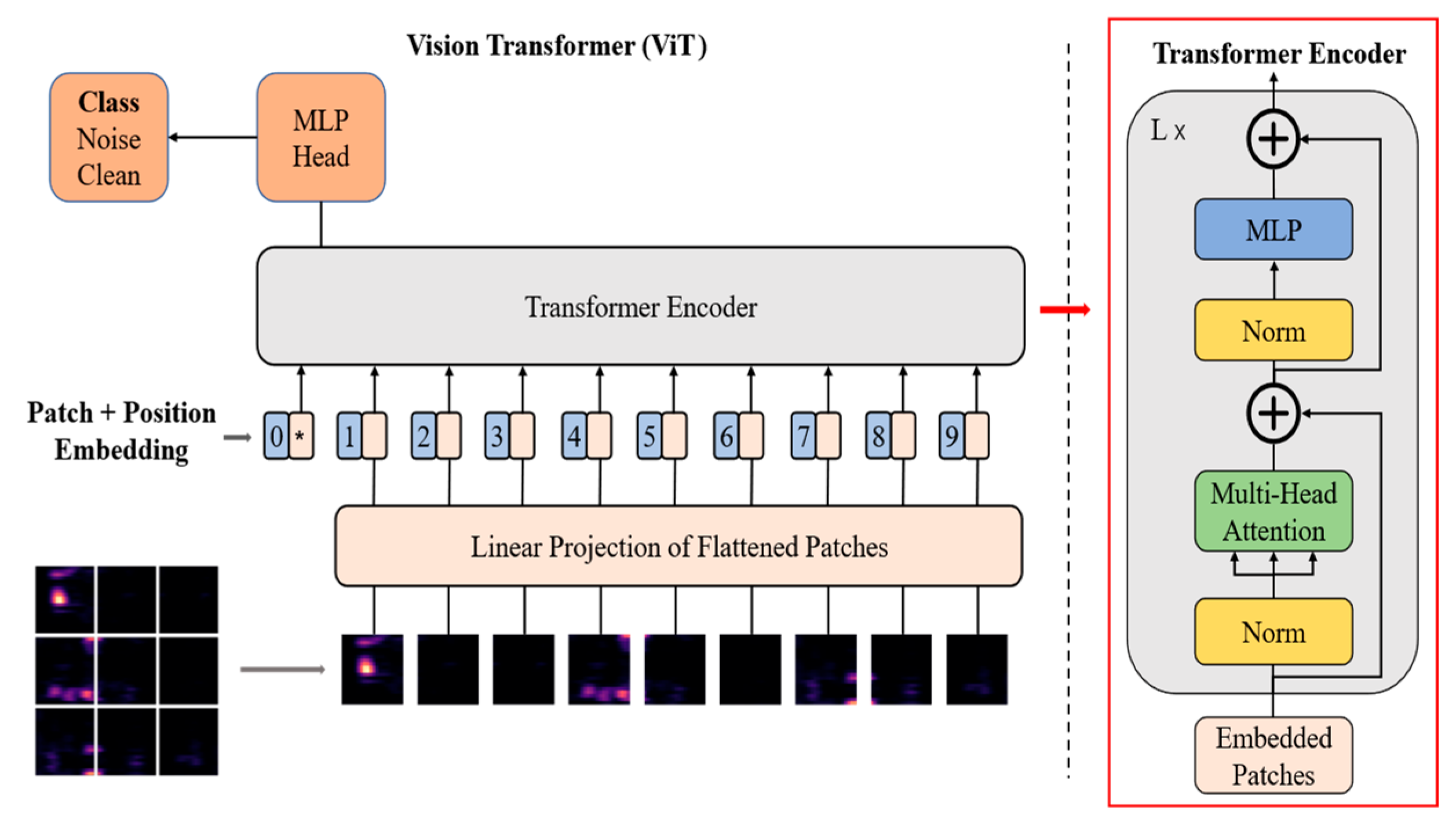
2.3. Network Structure
3. Experimental Results
3.1. Data Preparation
3.2. Comparison Method
3.3. Training and Test
4. Identification Results to Support Noise Attenuation
5. Conclusions
Author Contributions
Funding
Institutional Review Board Statement
Informed Consent Statement
Data Availability Statement
Conflicts of Interest
Abbreviations
| QC | Quality control |
| ViT | Vision Transformer |
| CNNs | Convolutional neural networks |
| RNNs | Recurrent neural networks |
| STFT | Short-Time Fourier Transform |
| MSA | Multi-Head Self-Attention |
| MLP | Multilayer Perceptron |
| Q | Query |
| K | Key |
| V | Value |
| ReLU | Rectified linear unit |
| SNR | Signal-to-noise ratio |
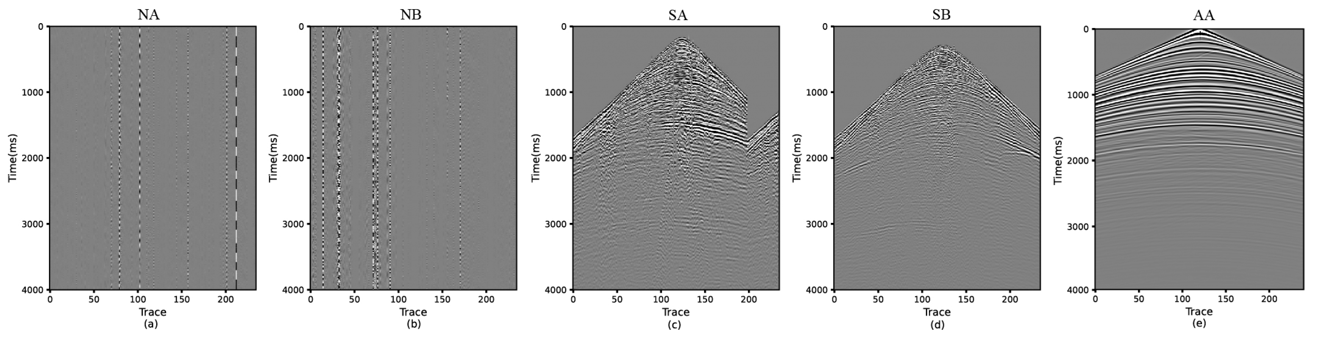
| NA | Noise Data A |
| NB | Noise Data B |
| SA | Seismic Data A |
| SB | Seismic Data B |
| AA | Acoustic Data A |
| AAA | Anomalous Amplitude Attenuation |
References
- Li, X.; Qi, Q.; Yang, Y.; Duan, P.; Cao, Z. Removing Abnormal Environmental Noise in Nodal Land Seismic Data Using Deep Learning. Geophysics 2024, 89, WA143–WA156. [Google Scholar] [CrossRef]
- Mao, X.; Yang, W.; Pang, Z.; Zhou, Q.; Mao, H.; Zhang, D.; Wang, X.; Pan, L. Combined Identification and Attenuation of Anomalous Amplitude Noises in Nodal Land Seismic Data. Front. Earth Sci. 2025, 13, 1535990. [Google Scholar] [CrossRef]
- Tian, X.; Cai, C.; Qu, W.; Meng, X.; Lu, J. Research and Application of the Relationship between Wireless Node Status QC and Seismic Data Quality. Geophys. Prospect. Pet. 2024, 63, 735–745. [Google Scholar] [CrossRef]
- Zou, S. Research and Application of Quality Monitoring Technology Based on Node Instrument Data Acquisition. Prog. Geophys. 2024, 39, 1493–1500. [Google Scholar] [CrossRef]
- Evans, B.J. A Handbook for Seismic Data Acquisition in Exploration; Society of Exploration Geophysicists: Tulsa, Okla, 1997; ISBN 978-1-56080-041-5. [Google Scholar]
- Tian, X.; Lu, W.; Li, Y. Improved Anomalous Amplitude Attenuation Method Based on Deep Neural Networks. IEEE Trans. Geosci. Remote Sens. 2022, 60, 1–11. [Google Scholar] [CrossRef]
- Li, X.; Qi, Q.; Wang, T.; Zhang, D. Removing Anomalous Noise from Seismic Data. In Proceedings of the SEG 1st Tarim Ultra-Deep Oil & Gas Exploration Technology Workshop, Korla, China, 3–5 June 2024; Society of Exploration Geophysicists: Tulsa, Okla, 2024; pp. 181–184. [Google Scholar]
- Song, C.; Liu, Z.; Wang, Y.; Li, X.; Hu, G. Multi-Waveform Classification for Seismic Facies Analysis. Comput. Geosci. 2017, 101, 1–9. [Google Scholar] [CrossRef]
- Roksandić, M.M. Seismic Facies Analysis Concepts. Geophys. Prospect. 1978, 26, 383–398. [Google Scholar] [CrossRef]
- Coléou, T.; Poupon, M.; Azbel, K. Unsupervised Seismic Facies Classification: A Review and Comparison of Techniques and Implementation. Lead. Edge 2003, 22, 942–953. [Google Scholar] [CrossRef]
- Xu, G.; Haq, B.U. Seismic Facies Analysis: Past, Present and Future. Earth-Sci. Rev. 2022, 224, 103876. [Google Scholar] [CrossRef]
- Chen, C.H. Seismic Pattern Recognition. Geoexploration 1978, 16, 133–146. [Google Scholar] [CrossRef]
- Tjøstheim, D. Improved Seismic Discrimination Using Pattern Recognition. Phys. Earth Planet. Inter. 1978, 16, 85–108. [Google Scholar] [CrossRef]
- Ming, Z.; Shi, C.; Yuen, D. Waveform Classification and Seismic Recognition by Convolution Neural Network. Chin. J. Geophys. 2019, 62, 374–382. [Google Scholar] [CrossRef]
- Amendola, A.; Gabbriellini, G.; Dell’Aversana, P.; Marini, A.J. Seismic Facies Analysis through Musical Attributes. Geophys. Prospect. 2017, 65, 49–58. [Google Scholar] [CrossRef]
- Xie, T.; Zheng, X.; Zhang, Y. Seismic Facies Analysis Based on Speech Recognition Feature Parameters. Geophysics 2017, 82, O23–O35. [Google Scholar] [CrossRef]
- Anderson, R.G.; McMECHAN, G.A. Automatic Editing of Noisy Seismic Data. Geophys. Prospect. 1989, 37, 875–892. [Google Scholar] [CrossRef]
- Shen, S.; Wang, B.; Zeng, L.; Chen, S.; Xie, L.; She, Z.; Huang, L. Methods for Identifying Effective Microseismic Signals in a Strong-Noise Environment Based on the Variational Mode Decomposition and Modified Support Vector Machine Models. Appl. Sci. 2024, 14, 2243. [Google Scholar] [CrossRef]
- Shakeel, M.; Nishida, K.; Itoyama, K.; Nakadai, K. 3D Convolution Recurrent Neural Networks for Multi-Label Earthquake Magnitude Classification. Appl. Sci. 2022, 12, 2195. [Google Scholar] [CrossRef]
- Di, H.; Shafiq, M.; AlRegib, G. Multi-Attribute k-Means Clustering for Salt-Boundary Delineation from Three-Dimensional Seismic Data. Geophys. J. Int. 2018, 215, 1999–2007. [Google Scholar] [CrossRef]
- Song, C.; Li, L.; Li, L.; Li, K. Robust K-Means Algorithm with Weighted Window for Seismic Facies Analysis. J. Geophys. Eng. 2021, 18, 618–626. [Google Scholar] [CrossRef]
- Troccoli, E.B.; Cerqueira, A.G.; Lemos, J.B.; Holz, M. K-Means Clustering Using Principal Component Analysis to Automate Label Organization in Multi-Attribute Seismic Facies Analysis. J. Appl. Geophys. 2022, 198, 104555. [Google Scholar] [CrossRef]
- Köhler, A.; Ohrnberger, M.; Scherbaum, F. Unsupervised Pattern Recognition in Continuous Seismic Wavefield Records Using Self-Organizing Maps. Geophys. J. Int. 2010, 182, 1619–1630. [Google Scholar] [CrossRef]
- Saraswat, P.; Sen, M.K. Artificial Immune-Based Self-Organizing Maps for Seismic-Facies Analysis. Geophysics 2012, 77, O45–O53. [Google Scholar] [CrossRef]
- Du, H.; Cao, J.; Xue, Y.; Wang, X. Seismic Facies Analysis Based on Self-Organizing Map and Empirical Mode Decomposition. J. Appl. Geophys. 2015, 112, 52–61. [Google Scholar] [CrossRef]
- Liu, Z.; Cao, J.; Chen, S.; Lu, Y.; Tan, F. Visualization Analysis of Seismic Facies Based on Deep Embedded SOM. IEEE Geosci. Remote Sens. Lett. 2021, 18, 1491–1495. [Google Scholar] [CrossRef]
- Alaudah, Y.; Michałowicz, P.; Alfarraj, M.; AlRegib, G. A Machine-Learning Benchmark for Facies Classification. Interpretation 2019, 7, SE175–SE187. [Google Scholar] [CrossRef]
- Liu, M.; Jervis, M.; Li, W.; Nivlet, P. Seismic Facies Classification Using Supervised Convolutional Neural Networks and Semisupervised Generative Adversarial Networks. Geophysics 2020, 85, O47–O58. [Google Scholar] [CrossRef]
- Zhang, H.; Chen, T.; Liu, Y.; Zhang, Y.; Liu, J. Automatic Seismic Facies Interpretation Using Supervised Deep Learning. Geophysics 2021, 86, IM15–IM33. [Google Scholar] [CrossRef]
- Chikhaoui, K.; Alfarraj, M. Self-Supervised Learning for Efficient Seismic Facies Classification. Geophysics 2024, 89, IM61–IM76. [Google Scholar] [CrossRef]
- Chai, X.; Nie, W.; Lin, K.; Tang, G.; Yang, T.; Yu, J.; Cao, W. An Open-Source Package for Deep-Learning-Based Seismic Facies Classification: Benchmarking Experiments on the SEG 2020 Open Data. IEEE Trans. Geosci. Remote Sens. 2022, 60, 1–19. [Google Scholar] [CrossRef]
- You, J.; Zhao, J.; Huang, X.; Zhang, G.; Chen, A.; Hou, M.; Cao, J. Explainable Convolutional Neural Networks Driven Knowledge Mining for Seismic Facies Classification. IEEE Trans. Geosci. Remote Sens. 2023, 61, 1–18. [Google Scholar] [CrossRef]
- Yang, N.-X.; Li, G.-F.; Li, T.-H.; Zhao, D.-F.; Gu, W.-W. An Improved Deep Dilated Convolutional Neural Network for Seismic Facies Interpretation. Pet. Sci. 2024, 21, 1569–1583. [Google Scholar] [CrossRef]
- dos Santos, D.T.; Roisenberg, M.; dos Santos Nascimento, M. Deep Recurrent Neural Networks Approach to Sedimentary Facies Classification Using Well Logs. IEEE Geosci. Remote Sens. Lett. 2022, 19, 1–5. [Google Scholar] [CrossRef]
- Zhou, Y.; Chen, W. Recurrent Autoencoder Model for Unsupervised Seismic Facies Analysis. Interpretation 2022, 10, T451–T460. [Google Scholar] [CrossRef]
- Wang, Z.; Wang, Q.; Yang, Y.; Liu, N.; Chen, Y.; Gao, J. Seismic Facies Segmentation via a Segformer-Based Specific Encoder–Decoder–Hypercolumns Scheme. IEEE Trans. Geosci. Remote Sens. 2023, 61, 1–11. [Google Scholar] [CrossRef]
- Huo, J.; Liu, N.; Xu, Z.; Wang, X.; Gao, J. Seismic Facies Classification Using Label-Integrated and VMD-Augmented Transformer. IEEE Trans. Geosci. Remote Sens. 2024, 62, 1–10. [Google Scholar] [CrossRef]
- Zhou, L.; Gao, J.; Chen, H. Seismic Facies Classification Based on Multilevel Wavelet Transform and Multiresolution Transformer. IEEE Trans. Geosci. Remote Sens. 2025, 63, 1–12. [Google Scholar] [CrossRef]
- Zhang, T.; Feng, G.; Liang, J.; An, T. Acoustic Scene Classification Based on Mel Spectrogram Decomposition and Model Merging. Appl. Acoust. 2021, 182, 108258. [Google Scholar] [CrossRef]
- Ustubioglu, A.; Ustubioglu, B.; Ulutas, G. Mel Spectrogram-Based Audio Forgery Detection Using CNN. Signal Image Video Process. 2023, 17, 2211–2219. [Google Scholar] [CrossRef]
- Sinha, S.; Routh, P.S.; Anno, P.D.; Castagna, J.P. Spectral Decomposition of Seismic Data with Continuous-Wavelet Transform. Geophysics 2015, 70, P19–P25. [Google Scholar] [CrossRef]
- Chakraborty, A.; Okaya, D. Frequency-time Decomposition of Seismic Data Using Wavelet-based Methods. Geophysics 1995, 60, 1906–1916. [Google Scholar] [CrossRef]
- Dosovitskiy, A.; Beyer, L.; Kolesnikov, A.; Weissenborn, D.; Zhai, X.; Unterthiner, T.; Dehghani, M.; Minderer, M.; Heigold, G.; Gelly, S.; et al. An Image Is Worth 16x16 Words: Transformers for Image Recognition at Scale. arXiv 2020, arXiv:2010.11929. [Google Scholar]
- Sun, L.; Zheng, X.; Ding, L.; Shou, H.; Li, H. Automatic Identification of Strong Energy Noise in Seismic Data Based on U-Net. IEEE Trans. Geosci. Remote Sens. 2023, 61, 1–11. [Google Scholar] [CrossRef]


| Method | Type | Accuracy Rate | Overall Accuracy Rate |
|---|---|---|---|
| Mel-spectrogram | Weak noise | 90.2% | 89.2% |
| Strong noise | 82.5% | ||
| Raw seismic trace | Weak noise | 94.7% | 94.5% |
| Strong noise | 93.1% |
Disclaimer/Publisher’s Note: The statements, opinions and data contained in all publications are solely those of the individual author(s) and contributor(s) and not of MDPI and/or the editor(s). MDPI and/or the editor(s) disclaim responsibility for any injury to people or property resulting from any ideas, methods, instructions or products referred to in the content. |
© 2025 by the authors. Licensee MDPI, Basel, Switzerland. This article is an open access article distributed under the terms and conditions of the Creative Commons Attribution (CC BY) license (https://creativecommons.org/licenses/by/4.0/).
Share and Cite
Ding, Q.; Chen, S.; Shen, J.; Wang, B. Identification of Environmental Noise Traces in Seismic Recordings Using Vision Transformer and Mel-Spectrogram. Appl. Sci. 2025, 15, 8586. https://doi.org/10.3390/app15158586
Ding Q, Chen S, Shen J, Wang B. Identification of Environmental Noise Traces in Seismic Recordings Using Vision Transformer and Mel-Spectrogram. Applied Sciences. 2025; 15(15):8586. https://doi.org/10.3390/app15158586
Chicago/Turabian StyleDing, Qianlong, Shuangquan Chen, Jinsong Shen, and Borui Wang. 2025. "Identification of Environmental Noise Traces in Seismic Recordings Using Vision Transformer and Mel-Spectrogram" Applied Sciences 15, no. 15: 8586. https://doi.org/10.3390/app15158586
APA StyleDing, Q., Chen, S., Shen, J., & Wang, B. (2025). Identification of Environmental Noise Traces in Seismic Recordings Using Vision Transformer and Mel-Spectrogram. Applied Sciences, 15(15), 8586. https://doi.org/10.3390/app15158586