1. Introduction
With the growing demand for customized and small-batch diversified production, the traditional “dedicated pipeline for dedicated tasks” operation model in edible oil factories is no longer sufficient to meet the requirements of modern manufacturing. Consequently, improving the efficiency of scheduling and planning in pipeline transportation systems has become a critical challenge in production management. Ensuring timely delivery while minimizing pipeline equipment usage to shorten order fulfillment time has become an urgent challenge for the edible oil industry.
In response to increasing demands for high customization, rapid order fulfillment, and small-batch diversified production, the scheduling volume of edible oil transportation tasks has grown significantly. However, each task is typically subject to strict time constraints. As a result, the efficient allocation of pipeline segments, valves, and other resources has become a critical challenge in transportation scheduling. Dynamic allocation of pipeline and valve resources shortens edible oil delivery time and balances resource efficiency with task prioritization, thereby enhancing operational performance.
Currently, traditional edible oil transportation factories still rely heavily on the manual operation of complex pipeline systems, which gives rise to the following common issues:
Low efficiency in pipeline and valve resource allocation due to the lack of holistic planning, often resulting in equipment idleness or resource conflicts;
Absence of real-time dispatching and visual monitoring systems, making it difficult to respond flexibly to task changes, thereby causing scheduling confusion and operational delays;
Poor integration between scheduling decisions and on-site operations, which reduces responsiveness and system stability;
Heavy reliance on operator experience for determining pipeline switching sequences, which increases the risk of production downtime or operational errors when facing production changes or unexpected events, thus raising transportation costs;
Labor shortages caused by an aging workforce, further complicating system management and disrupting operational continuity
This study introduces an intelligent and automated scheduling assistance mechanism and establishes a multi-objective optimization decision-making system to enhance the overall planning efficiency of edible oil transportation tasks. The proposed digital management framework integrates internal pipeline data from the factory, thereby reinforcing the digitization and intelligent control of the pipeline transport system. The system is developed using the C# programming language. The system incorporates a path planning algorithm, SolidWorks Professional, for pipeline modeling, and the Helix Toolkit V2.24.0 for 3D simulation, forming a comprehensive intelligent scheduling platform. Beyond its 3D visualization features, the interface design incorporates the Helix Toolkit V2.24.0 and SolidWorks Professional, allowing operators to accurately interpret the pipeline scheduling status. This integration enhances execution precision and facilitates real-time operational adjustments. The path planning algorithm serves as the core of the optimization process, supporting factory managers in making safer and more efficient scheduling decisions.
The main contributions of this study are as follows:
Development of a multi-objective optimization scheduling system for edible oil transportation: The proposed system addresses scheduling challenges by establishing a mechanism that balances pipeline resource utilization efficiency, effectively avoiding resource idleness or overuse and reducing overall operational costs;
Implementation of a dynamic path planning mechanism: In response to unexpected events, such as valve failures or urgent task insertions, the system is capable of promptly recalculating alternative routes to ensure the continuity and stability of edible oil delivery operations;
Design of a digital twin-based 3D visual human–machine interface: By intuitively presenting pipeline scheduling results through visual representations, the interface supports deployment in digital factory environments and improves the decision-making efficiency and accuracy of on-site operators;
Validation of effectiveness and operational improvement: The proposed method achieves high scheduling performance in both simulation and real-world experiments, with up to a 43% improvement in scheduling efficiency and notable enhancements in pipeline transportation system performance.
2. Related Work
This section reviews the existing studies in the domains of path planning algorithms, multi-objective optimization techniques, pipeline transportation scheduling and optimization, and the automation of traditional edible oil factory operations. These prior works collectively establish a solid theoretical foundation for the system architecture and implementation strategies proposed in this study.
2.1. Path Planning Algorithm
The shortest path problem in pipeline transportation systems has long been a central topic in academic research, and is widely applied in Pipe Routing Design (PRD). Classical algorithms, such as Dijkstra’s algorithm [
1], the A* algorithm [
2], and maze-solving algorithms [
3], have been extensively studied. These methods predominantly adopt greedy strategies to solve shortest-path problems on graph-based structures. Specifically, Dijkstra’s algorithm systematically explores all possible paths from a source node to determine the global shortest path, making it particularly suitable for accurate searches in static environments. The A* algorithm improves search efficiency by incorporating heuristic functions while maintaining solution optimality. Maze-solving algorithms, on the other hand, emulate human exploratory behavior in complex environments and are especially effective for spatial navigation involving obstacles. In static environments, the Dijkstra algorithm demonstrates both high computational efficiency and accuracy [
4]. This characteristic makes it particularly suitable for solving logistics route optimization problems, effectively addressing various challenges in transportation networks [
5]. Furthermore, by incorporating real-time traffic flow data as edge weights, the algorithm can adapt to dynamic road conditions, such as traffic congestion and road closures, resulting in improved routing performance [
6].
In this context, the A* algorithm plays a central role in the present study. For example, [
7] proposed a routing methodology for automated ship pipeline configurations by integrating an enhanced A* algorithm with genetic algorithms, significantly improving pipe layout efficiency and system automation. Similarly, [
8] refined the heuristic function of the conventional A* algorithm to accommodate cleaning and disinfection service robots, thereby ensuring path continuity and operational safety. With ongoing advances in smart manufacturing and digital factories, recent studies have extended shortest-path techniques to complex scenarios, such as multi-layer spaces, dynamic obstacles, and time window constraints. These developments not only enhance the robustness and adaptability of pathfinding algorithms in real-world applications but strengthen their capabilities in intelligent decision-making and real-time scheduling.
2.2. Multi-Objective Optimization Methods
Multi-objective optimization is a subfield of mathematical optimization that simultaneously addresses the optimization of multiple objective functions. In multi-objective problems, objectives are considered conflicting if the improvement of one objective results in the deterioration of others. A solution is defined as Pareto optimal, Pareto efficient, or non-dominated if no alternative solution exists that can improve one objective without compromising at least one other. Non-dominated solutions serve as a fundamental criterion for evaluating the quality of the solution set. Specifically, the Pareto optimal set consists of solutions for which no objective can be further improved without compromising another [
9]. In practical applications, multi-objective optimization is widely employed in areas such as engineering design, resource allocation, and scheduling optimization. It provides decision-makers with a diverse and flexible set of solutions, enabling effective trade-offs among competing objectives.
The Pareto front partitions the objective function space into feasible and infeasible regions in multi-objective optimization problems. It is defined as the boundary encompassing all feasible points that satisfy the constraints, representing the set of optimal trade-off solutions [
10,
11]. Depending on the number of objectives, the Pareto front can manifest as a continuous curve in two-objective problems or as a multidimensional surface in higher-dimensional spaces. Constructing and analyzing the Pareto set facilitates the effective balancing of conflicting objectives, thereby providing a rigorous scientific foundation for decision-making.
Multi-objective evolutionary algorithms (MOEAs) have been widely applied to shortest path problems, exhibiting strong capabilities in maintaining solution diversity while managing computational complexity [
12]. To overcome challenges such as the limitations of the Pareto dominance criteria, methods including quartile filtering combined with penalty mechanisms have been proposed to achieve a balance between convergence and diversity [
13]. Furthermore, enhanced Dijkstra’s and Floyd’s algorithms have been applied in emergency logistics transportation to model practical constraints, enabling Pareto front generation and providing real-time decision support [
14].
2.3. Pipeline Transportation System Scheduling
Scheduling in pipeline transportation systems can be broadly categorized into static and dynamic scheduling. Static scheduling establishes the task sequence and timing at the initial stage, resulting in a relatively straightforward process; however, due to its rigidity, it is often incapable of responding effectively to unexpected changes or anomalies. By contrast, dynamic scheduling adapts task sequences, transportation routes, and related plans in real time based on up-to-date information and specific conditions [
15]. Research on scheduling methodologies generally falls into four main categories: mathematical programming, simulation optimization, heuristic algorithms, and machine learning. Among these, mathematical optimization techniques have been extensively studied in the literature [
16,
17,
18], and the associated scheduling problems have been proven to be NP-hard [
19]. Consequently, many studies have employed heuristic algorithms to improve the computational efficiency of mathematical programming approaches [
20]. Simulation optimization, which models dynamic system environments and integrates dispatching rules for performance evaluation, has been widely applied in practical settings [
21]. Additionally, machine learning techniques have been leveraged for predicting operation durations, identifying bottlenecks, and autonomously adjusting schedules.
In the context of pipeline transportation, approaches based on mathematical programming and heuristic algorithms have been proposed, including the precise modeling of internal fluid flow to improve pipeline stability and efficiency [
22]. The developed decision support system (DSS) framework aims to advance pipeline transportation optimization by improving throughput capacity, optimizing schedules to reduce total transportation time, and incorporating buffering mechanisms [
23]. Additionally, an automated pipeline design system integrated within a CAD environment was introduced, employing network optimization to develop pipeline routing systems [
24]. In crude oil scheduling, smart field (SF) technologies have been utilized to reduce oil switching frequency, thereby decreasing transportation costs [
25]. Furthermore, a hybrid modeling approach combining mechanical and data-driven models was proposed to predict the operating parameters of oil and gas pipelines, facilitating optimized scheduling decisions [
26]. Ref. [
27] proposed a novel scheduling framework utilizing Boolean satisfiability (SAT) and mixed integer programming (MIP) methods. Within this framework, schedulers must make real-time decisions based on partial information, lacking full knowledge of future tasks or constraints. This approach addresses the challenge of effectively allocating limited resources amid continuously changing and uncertain conditions.
3. Edible Oil Pipeline Model and System
In practical factory operations, task allocation is centrally managed by a control center; therefore, this study adopts a centralized scheduling approach for system design. A 3D factory model simulating the actual oil transportation environment was developed and employed for experiments and testing. The edible oil factory contains multiple storage tanks, some of which are dedicated to storing specific types of oil, while others serve as temporary storage facilities to ensure the safety and quality of the stored products. Pipelines equipped with transport systems connect these storage tanks, allowing flexible adjustments of oil transportation routes according to production tasks.
3.1. Three-Dimensional Model of the Edible Oil Transportation Plant
The edible oil processing plant is equipped with multiple storage tanks, some of which are designated for specific types of edible oils, while others serve as temporary storage units to ensure the quality and safety of the oil during storage. Pipelines connect the storage tanks to facilitate the transfer of edible oils throughout the facility. This pipeline system is highly flexible and can be dynamically reconfigured based on production requirements, supporting real-time scheduling and accommodating high-mix, low-volume manufacturing demands. Such adaptability enhances transportation efficiency and operational flexibility.
The plant incorporates various edible oil transfer components, including valves, regulators, pipelines, and storage tanks.
Figure 1 presents an aerial view of the facility, where the cylindrical tanks represent the storage units for edible oil materials. The plant is functionally divided into two main zones:
Main Edible Oil Storage Zone: This zone performs key operations such as receiving and temporarily storing incoming edible oil, transferring it to the packaging facility, dispatching for distribution, blending different oil types, and coordinating internal logistics, as shown in
Figure 2a. It also serves as the primary area for evaluating the proposed multi-objective scheduling optimization method;
Packaging Facility: As shown in
Figure 2b, this zone is responsible for bottling edible oil transported from the storage area, fulfilling order-specific blending requirements, and performing automated packaging to meet diverse and customized market demands.
As depicted in
Figure 2, the pipeline layout within the factory is highly complex. Currently, edible oil transfer tasks are manually coordinated by experienced operators who determine pipeline allocation and the sequential operation of valves. To prevent cross-contamination or pipeline overpressure, typically only one edible oil transfer task is performed at a time. While this approach reduces the risk of human error, it results in idle pipeline and valve resources, ultimately limiting production efficiency.
This study employed CAD software (SolidWorks Professional) to construct a 3D model of the factory and utilized the Helix Toolkit V2.24.0 for visualization and simulation. Prior to developing the 3D model, a comprehensive on-site survey of the factory’s pipeline system was conducted. Detailed information regarding pipelines, storage tanks, motors, valve switches, and other equipment was systematically recorded to establish a complete equipment inventory and mapping database. Based on this data, the pipelines and associated equipment were digitized to generate a digital map of the facility, providing comprehensive location details and operational status, as illustrated in
Figure 3. This digital foundation supports optimized path scheduling and integration with the automation system.
Furthermore, using accurate equipment models, dimensions, and pipeline layouts, the actual configuration of the edible oil transfer infrastructure was simulated, as shown in
Figure 4. The 3D visualization significantly enhances the intuitiveness and manageability of oil transfer operations by using color coding to distinguish between different transfer tasks. This allows managers to monitor valve and pipeline resources in real time for each task, facilitating a clearer understanding of the transportation process and improving scheduling accuracy and overall production efficiency.
3.2. Definition of Edible Oil Transfer Tasks
Given that edible oil transfer work orders typically comprise multiple task requirements, this study adopts a multi-objective optimization-based scheduling approach to determine the execution priorities of individual tasks. A set of critical parameters is first defined for each task, serving as the basis for priority evaluation. These parameters include factors such as task urgency, the type and volume of edible oil, and the current availability of relevant equipment and pipeline segments. By incorporating task prioritization, the proposed system efficiently allocates limited resources to optimize the execution sequence, thereby minimizing overall transportation time and improving operational efficiency. The key parameters considered in the scheduling of edible oil transportation tasks are as follows:
Task Objectives: The edible oil transportation tasks involve various routes, including transfers from tankers or refineries to large storage tanks, between different storage tanks, and from storage tanks to packaging plant tanks. Different tasks require corresponding transportation strategies to ensure smooth operation;
Edible Oil Types: Different edible oils have distinct viscosity characteristics and are stored in separate tanks. During transportation, special attention must be paid to avoid mixing and cross-contamination of edible oils;
Transportation Volume and Weight: In addition to the weight of the transported edible oil, the viscosity coefficient and density of the edible oil directly affect the transportation time and must be taken into account in calculations;
Source and Destination Tanks: Tanks in the large storage area are typically assigned to specific raw edible oil types, whereas those in the packaging plant area function as temporary storage for outbound oils, accommodating a wider and more variable range of oil types.
The parameters described above are defined based on the specific requirements of each edible oil transportation task, as summarized in
Table 1. In the task model, “T” denotes a storage tank, with the accompanying number representing its unique identifier;
3.3. Framework of the Edible Oil Transportation System
The framework of the edible oil transportation system, as illustrated in
Figure 5, is composed of four major modules, including Database Management and Design, Multi-Objective Optimization Decision Module, Scheduling Simulation Module, and Decision and System Integration Module.
Database Management and Design Module: This module is responsible for inventory tracking and management of key resources, including control valves, storage tanks, edible oil transport pipelines, and pump motors. It maintains records of quantity, location, and flow direction to ensure the availability and optimal allocation of resources within the system;
Multi-Objective Optimization Decision Module: This module employs pathfinding algorithms to determine the optimal pipeline route for each oil transport task. It dynamically identifies the required pipeline components and extracts relevant information from the valve and pipeline database. Based on this data, objective function scores and estimated transport times are calculated. A multi-objective optimization scheduling approach is then applied to assign priority levels to each task;
Scheduling Simulation Module: This module visualizes decision outcomes through 3D simulations. It outputs key performance indicators, such as transport duration, pipeline and equipment usage, optimal path distance, and computational time. These data support the decision-makers in monitoring execution status and assessing task performance in real time;
Decision-Making and System Integration Module: This module consolidates decision results from each transport task and provides scientific decision support for scheduling. The final scheduling results are transmitted to hardware components, such as PLCs (programmable logic controllers), enabling seamless integration with the physical edible oil transport system for automated task execution.
The primary contribution of this study lies in the application of multi-objective optimization theory to scheduling planning. By integrating this approach, the system is able to generate informed decision options and to achieve optimal allocation of resources and multitask execution. This method enables the maximization of transport efficiency through concurrent task execution while minimizing the overall completion time of work orders.
4. Multi-Objective Optimization for Edible Oil Transportation Scheduling Method
The essence of multi-objective optimization lies in balancing multiple evaluation criteria and making trade-offs among two or more conflicting objectives to achieve relatively optimal decision outcomes. In this study, the planned pipeline resource allocation determined using the A* and Dijkstra pathfinding algorithm is compared with the edible oil transportation time estimated via the Hagen–Poiseuille equation from fluid dynamics. Based on this comparison, each transportation task is evaluated and prioritized, forming the basis for the design of a multi-objective optimization scheduling algorithm.
4.1. Pareto Front
When numerous feasible solutions exist within the objective space, the Pareto front represents the boundary of solutions that satisfy all constraints, as illustrated by the red line in
Figure 6. This boundary represents the set of all potentially optimal solutions in a multi-objective optimization problem. In this study, two key evaluation criteria, pipeline resource utilization and edible oil transportation time, are used to compare and analyze various task scenarios. For instance, as shown in
Figure 6, although Task A consumes fewer pipeline resources (
f2), it requires a longer transportation time (
f1) compared to Task B. Conversely, Task B utilizes more resources but achieves a shorter transportation time. Achieving an optimal balance between transportation time and equipment usage is critical, as it directly influences the overall efficiency and performance of the scheduling system.
In pipeline scheduling for edible oil transportation, multi-objective optimization is employed to address the trade-off between pipeline resource utilization and transportation time. The core challenge lies in simultaneously achieving the following two objectives:
Minimization of the total cost based on pipeline node weights: The weight of a pipeline node represents its associated resource demand and operational complexity. Selecting nodes with lower weights helps reduce overall task costs and improves scheduling efficiency;
Minimization of edible oil transportation time: Reducing the transportation time directly enhances system throughput, which is particularly critical in handling urgent or high-priority tasks.
In the context of multi-objective optimization, a Pareto-optimal analysis based on pipeline node weight cost and transportation time is adopted to guide task prioritization and dynamic scheduling. The process consists of the following steps:
Pareto Front Analysis: Task cost (based on node weights) and transportation time are computed and displayed on a Pareto scatter plot. Points closer to the Pareto front indicate superior performance in both cost and time.
Multi-Objective Ranking and Decision Mechanism: When the cost difference between the top-ranked task and the rest is below a predefined threshold wcost, the system further evaluates whether the top task also has the shortest transportation time.
- (a)
If the highest-ranked task does not have the shortest transportation time, the system reassigns priority to the task with the minimum delivery time and updates the scheduling order accordingly;
- (b)
This decision-making process jointly considers pipeline cost and transportation efficiency, ensuring a balanced trade-off between operational performance and resource utilization.
The integration of multi-objective optimization theory into real-world edible oil pipeline scheduling introduces a dynamic and scientifically grounded scheduling framework. This approach addresses the shortcomings of traditional single-objective strategies, which often lead to inefficiencies and resource underutilization. It is particularly effective in complex factory environments characterized by variable task requirements and high-priority constraints.
4.2. Dijkstra’s Path Planning Algorithm
Dijkstra’s algorithm is a greedy-based pathfinding method that iteratively selects the node with the smallest current distance for expansion. It is applicable to graph structures without negative edge weights. The computational procedure of the algorithm is as follows [
29]:
- 2.
Current Node Selection: Select an unvisited node n with the smallest tentative distance d(n) and mark it as visited;
- 3.
Distance Update: For each neighbor node m adjacent to node n, if the distance d(m) from the starting node A to m via n can be shortened, update it as follows:
where
d(n) represents the current shortest distance from node A to node n,
d(m) is the currently known shortest distance to node m, and
w(n,m) denotes the edge weight (distance) between nodes n and m;
- 4.
Mark node n as processed. Repeat steps 2 and 3 until all nodes have been visited.
4.3. A* Path Planning Algorithm
Prior to executing the multi-objective scheduling optimization, a dedicated shortest path must be determined for each individual task. Once the shortest path information is obtained, it enables further evaluation of the required pipeline resources and total transportation time for task execution. The system iteratively runs the path planning algorithm to identify the next task for the multi-objective scheduling until no feasible paths remain for any outstanding tasks.
In this study, all edges in the factory map are considered directed and non-negative. Due to the specific production requirements of edible oil transportation pipelines, certain nodes impose directional constraints to prevent backflow, such as unidirectional designs in specific tanks, valves, and pipeline sections. Based on these characteristics and constraints, the A* algorithm was selected as the core path planning method. The A* algorithm employs a heuristic search strategy to efficiently identify the optimal path by combining the actual cost from the start node to the current node with the estimated cost from the current node to the goal [
29].
The value for
f(n) represents the estimated total cost from the start node A to node n, combining both the actual cost incurred and the estimated cost to reach the goal.
The value for
g(n) denotes the actual cost from the start node A to node n, where
cost(A, n) is the actual movement cost along the path from A to n.
The value for
h(n) is the heuristic estimate of the cost from node n to the goal node, often computed as the Euclidean distance and serving as the heuristic function value.
For each neighboring node n of the current starting node A, perform the following node expansion rules:
Compute the actual cost from the starting node A to node n, denoted as Equation (4);
Estimate the heuristic cost from node n to the target node, denoted as Equation (5);
Calculate the total cost of node n as Equation (3).
If node n is not yet included in the open list, it is added. If node n is already present in the open list, its f-value is updated accordingly to reflect the improved path cost.
4.4. Pipeline Cost Function
During the digitization of the pipeline system, special attention must be given to the unique nature of edible oil transport, particularly the need to prevent edible oil cross-contamination. In this study, directional indicators were assigned to each node to reflect its functional role, as illustrated in
Figure 7. Arrows pointing outward indicate edible oil outflow, whereas those pointing inward denote edible oil inflow. To quantify the scheduling significance of each node, we define the “node connectivity number” as the total count of its outward connections. This number serves as an indicator of the node’s potential for flow distribution. Nodes with higher connectivity are more likely to be frequently utilized in edible oil transfer operations and may become bottlenecks, leading to congestion of pipeline resources. Accordingly, node connectivity is incorporated as a weighted parameter in the scheduling algorithm. In practical applications, critical nodes are often cross-type junctions with four outlets. Therefore, the upper bound of node weight
wcost is set to 4 in this study, serving as a reference for prioritizing scheduling decisions.
In the proposed system design, the shortest path for each edible oil transfer task is first computed using a path planning algorithm. The total cost is then obtained by summing the weight values of all nodes, such as valves and pipes, encountered along the path. Node weights are assigned based on their connectivity (i.e., the number of links to other nodes) to control their frequency of usage during scheduling. Nodes with higher connectivity are assigned to a lower scheduling priority, which helps reduce resource congestion at highly connected junctions. This strategy promotes balanced utilization of pipeline resources and enhances the system’s ability to handle dynamic and highly variable operational demands.
Due to differences in node position and function, the number of links varies between nodes, influencing their assigned cost weight. To prevent high-flexibility nodes, such as multi-directional valves or frequently used pipe junctions from becoming over utilized by a single task, a node weight-limiting mechanism is introduced. As illustrated in the A* path planning example in
Figure 8, the specific valve and pipeline resources used during the routing process are analyzed. The connectivity and weight of each node are summarized in
Table 2, with different node types visually distinguished using color coding. Furthermore, as shown in
Table 2, the parameters for pipeline resources required by each task are relatively well-defined. The factory’s oil transportation task planning is conducted based on customer order requirements, with task contents generally being quite explicit.
Moreover, the complexity of the oil pipeline environment is significantly lower compared to the movement paths and environments encountered by robots or autonomous mobile robots (AMRs).
The proposed cost function is calculated based on the number of nodes traversed by each task and their associated weights. This function serves as the basis for determining the execution priority of individual edible oil transfer tasks. The cost function for pipeline scheduling is defined as follows:
where
TTask is the total number of connected nodes corresponding to all edible oil storage tanks along the planned path;
PiTask is the total number of connected nodes for all pipeline segments traversed in the path;
VTask is the total number of connected nodes related to valves encountered during routing;
PuTask, in path planning, is the total number of nodes connected to all pumps is considered. This node count also takes energy consumption into account, with weights adjusted based on the pump power;
EmTask is the urgency level set by the decision-maker reduces the objective function value, thereby increasing the priority of the task. By default, the urgency is unknown. Urgent events include situations such as failures and maintenance.
When multiple tasks are scheduled concurrently, tasks with lower pipeline costs are prioritized. This strategy maximizes the utilization of available resources and minimizes scheduling conflicts arising from contention for shared equipment.
4.5. Edible Oil Transportation Time Function
In the production process of edible oil plants, transportation time is a critical factor for scheduling and operational efficiency. This study estimates the transportation time of various edible oils based on the Hagen–Poiseuille law, which describes fluid flow through pipelines, and utilizes these estimations to arrange production sequences accordingly. The physical properties of edible oils, especially their viscosity coefficients, significantly affect their transit times within the pipelines. According to [
30], the viscosity and temperature characteristics vary among different types of edible oils, impacting flow behavior. Edible oils with higher viscosity require longer transportation times due to increased flow resistance, whereas those with lower viscosity can be transported faster under the same pipeline conditions. These differences impact not only the efficiency of individual transportation tasks but the overall scheduling and planning of production, especially in multi-product, multi-batch manufacturing scenarios. By accounting for the viscosity characteristics of edible oils in transport scheduling, the system effectively avoids prolonged transit times and pipeline congestion, thereby enhancing production efficiency and reducing operational costs [
30,
31,
32].
This study is conducted in a region characterized by a subtropical monsoon and tropical monsoon climate, with ambient temperatures fluctuating between approximately 15 °C and 35 °C. Accordingly, the viscosity coefficients of edible oils are standardized at an average temperature of around 25 °C, referencing 23.9 °C as reported in [
30]. Due to variations in oil density, conversions between mass and volume are required for relevant calculations. To ensure data consistency, this study adopts the density conversion values provided in [
33]. Based on the specified viscosity and density parameters, oil transport time is then calculated using fluid dynamics principles. Temperature also affects the viscosity coefficient of the oil. As temperature increases, the viscosity coefficient of edible oil typically decreases, resulting in increased fluidity; conversely, as temperature decreases, the viscosity coefficient increases, leading to reduced fluidity. According to the analysis presented in [
34], this study establishes a table correlating the viscosity coefficient of edible oil with temperature to enhance the accuracy of time function calculations. Specifically, the Hagen–Poiseuille law serves as the governing model to estimate the edible oil flow velocity v(m/s), incorporating pressure differential, pipe radius, viscosity coefficient, and pipe length as key variables [
35,
36]. The governing equation is defined as follows:
Here, Δ
P denotes the pressure difference between the two ends (Pa),
r is the pipeline radius (m),
η represents the viscosity coefficient of the edible oil (Pa·s), and
L is the total pipeline length required for the transportation task (m). This equation indicates that, as the viscosity coefficient increases, the flow velocity significantly decreases, thereby extending the transportation time. This physical property is a critical factor in edible oil transportation, since the viscosity can vary considerably among different oils. Consequently, differences in transportation time must be accounted for and adjusted within production scheduling. The actual transportation time of the edible oil can be further estimated using the volumetric flow rate formula, as follows:
where
Qv represents the volumetric flow rate (m
3/s),
A denotes the cross-sectional area of the pipeline (m
2),
V is the volume of the fluid (m
3), and
t is the time (min). By solving Equations (8) and (9) simultaneously, the relationship between volumetric flow rate and transportation time can be derived as follows:
Since different edible oils have varying densities, it is necessary to convert mass into volume. The calculation formula is as follows:
where
M represents mass, and
D denotes density. The cross-sectional area
A is defined as follows:
Next, substitute Equations (11) and (12) into Equation (10), then solve the system formed by Equations (10) and (7) simultaneously to calculate the transportation time
Ttask required for the edible oil transport task, as follows:
The scheduling of transportation time is based on the viscosity coefficients of edible oils, simulating their flow characteristics within the pipeline. For edible oils with different viscosities, the model can predict transport delays and adjust the scheduling sequence accordingly, providing decision-makers with a scientific basis for planning.
5. Experimental Results
This study integrates the scheduling decision system with the edible oil factory via a cyber-physical approach. By constructing a 3D model of the valve and pipeline network based on on-site inspections and incorporating task information provided by decision-makers, synchronized control and scheduling planning are realized. Experiments were conducted within an actual factory scheduling system performing task scheduling and execution. To avoid disrupting the operation of the oil transportation plant during testing, only a subset of isolated pipeline sections was selected for evaluation. Consequently, the number of tasks was limited, and the environment was relatively simple and well-defined. This section describes the 3D visualization experimental platform and interface, as well as the results of the multi-objective optimization decision-making process.
5.1. Experimental Platform
The experimental system combines multi-objective optimization scheduling algorithms with 3D visualization to display pipeline and task status in real time via the HMI, supporting dynamic adjustments and resource optimization (see
Figure 9a). The 3D model operation and control were developed using C# programming language, combined with an interactive HMI. Operators can rotate the model, respond to button commands, and simulate valve operations to realistically replicate the actual edible oil pipeline system’s operational scenarios. As shown in
Figure 9b, the HMI of the decision-making system includes sections for “New Tasks”, “Pending Tasks”, “Active Tasks”, and “Parameter Information”. It supports task input, list management, real-time status display, and system notifications for operations and task updates.
5.2. Experimental Results of Multi-Objective Optimization Scheduling
This study employs two scheduling methods, namely “Multi-Objective Optimization” and “First-In-First-Out (FIFO)” to schedule edible oil transportation work orders, and compares the efficiency of the resulting schedules. In the multi-objective optimization approach, for each scheduling iteration, the A* and Dijkstra path planning algorithm are used to calculate the shortest path for each task. The pipeline node weights involved in transporting the edible oil are then aggregated to compute the corresponding cost function. Concurrently, a time function for each task is calculated based on the route and the type of edible oil. These cost and time functions are then used to generate a two-dimensional Pareto distribution plot, facilitating the identification of the Pareto front for each scheduling solution. This process iteratively optimizes the task prioritization to achieve improved scheduling. By contrast, the FIFO method strictly adheres to the first-in-first-out principle, executing two tasks per scheduling round. To prevent pipeline conflicts and oil mixing, each task must be fully completed before the next can begin.
The experiments analyzed work orders under four different scenarios:
Fixed edible oil weight: All variables remain constant, including edible oil weight and task priority;
Variable edible oil weight: Simulates the impact of different edible oil weights on scheduling. As the edible oil weight increases or decreases, the system dynamically adjusts pipeline resource allocation to meet varying production demands;
Fixed edible oil weight with emergency task constraints: Introduces emergency tasks with specific priorities and time constraints. The system must promptly adjust the existing schedule to prioritize completion of emergency tasks;
Variable edible oil weight with emergency task constraints: Combines edible oil weight fluctuations and emergency tasks. The system must complete emergency tasks for underweight constraints while maintaining the normal operation of other tasks.
Each scenario involves eight tasks per work order, with task sequences randomly arranged. The source of each task contains specific edible oil types, while destinations are randomly matched to either temporary storage tanks or packaging plant tanks. The goal is to transport edible oil to the designated destinations until all tasks are completed.
5.2.1. Fixed Edible Oil Weight
In this scenario, the work orders are as shown in
Table 3, where all variables remain constant, including the edible oil weight and task priorities. The objective is to serve as a baseline test for evaluating the scheduling performance under static conditions.
First, scheduling and analysis were performed using a multi-objective optimization approach that incorporated both the A* algorithm and Dijkstra’s algorithm. The Pareto front obtained from the first scheduling iteration is shown in
Figure 10a, where the horizontal axis represents the cost function and the vertical axis represents the time function. In the case of the A* algorithm, Task 8 appeared on the Pareto front, marked by a red “◎”. Likewise, in the Dijkstra algorithm result, Task 8 was also located on the Pareto front, indicated by a red “╳”. As a result, Task 8 was extracted from the job list and placed into the execution queue as the first task to be performed. The pipeline resources allocated to Task 8 were subsequently used as constraints for the scheduling of the remaining tasks. A second scheduling iteration was then conducted to determine the next optimal task.
As shown in
Figure 10b, the task distribution from the second scheduling iteration revealed that both the A* algorithm and Dijkstra’s algorithm identified Task 5 as the Pareto-optimal solution in this round. Therefore, Task 5 was added to the execution queue as the second task. The pipeline resources allocated to Tasks 8 and 5 were set as constraints for subsequent scheduling. In the third scheduling iteration, illustrated in
Figure 10c, the task distribution indicated that both the A* algorithm and Dijkstra’s algorithm selected Task 2 as the Pareto-optimal solution in this round. Accordingly, Task 2 was added to the execution queue as the third task. The pipeline resources allocated to Tasks 8, 5, and 2 were used as constraints for the subsequent scheduling iterations.
During the fourth scheduling iteration, depicted in
Figure 10d, the task distribution revealed that, for the A* algorithm, both Task 1 and Task 4 lay on the Pareto front. Among them, Task 1 required fewer pipeline resources than Task 4, while Task 4 had a shorter transportation time than Task 1. Although Task 1 involved fewer pipeline resources, its cost function value differed from that of Task 4 by less than 4. Since Task 1 did not have the shortest transportation time among the candidates, Task 4 was selected as the fourth task in the A* execution sequence. For Dijkstra’s algorithm, both Task 1 and Task 3 appeared on the Pareto front. After evaluation, Task 3 was selected as the fourth task. Additionally, due to the absence of an available oil pipeline path for Task 7, it was temporarily excluded from scheduling and is therefore not shown in
Figure 10d. The pipeline resources occupied by Tasks 8, 5, 2, and 4 were used as constraints for subsequent scheduling iterations under the A* algorithm, while those associated with Tasks 8, 5, 2, and 3 were set as constraints for Dijkstra’s algorithm.
The task distribution resulting from the fifth scheduling iteration is shown in
Figure 10e. For the A* algorithm, only Task 3 had an available oil pipeline path for execution; thus, Task 3 was added to the execution queue as the fifth task. Similarly, for Dijkstra’s algorithm, only Task 1 had an available oil pipeline path and was therefore assigned as the fifth task. At this point, there were temporarily no available pipeline resources. Consequently, the A* algorithm proceeded to execute oil transportation tasks for Tasks 8, 5, 2, 4, and 3 concurrently, while Dijkstra’s algorithm executed oil transportation tasks for Tasks 8, 5, 2, 3, and 1 simultaneously.
The sixth scheduling iteration entered a standby state, with Tasks 1, 6, and 7 remaining for the A* algorithm, and Tasks 4, 6, and 7 remaining for Dijkstra’s algorithm. Both algorithms awaited the completion of prior tasks and the release of pipeline resources. Upon resource availability, the path planning algorithms recalculated accessible routes and executed new oil transportation tasks accordingly. A subsequent task analysis indicated that none of the remaining tasks met the criteria to form a Pareto front. Therefore, the scheduling order from the sixth to the eighth iterations proceeded as follows: for the A* algorithm, Tasks 6, 1, and 7; for Dijkstra’s algorithm, Tasks 6, 4, and 7, as illustrated in
Figure 10f.
As shown in
Figure 11, a comparative summary of the execution sequences and time data between the multi-objective optimization scheduling method and the FIFO method for edible oil transportation tasks is presented. As shown in
Figure 11a, the A* algorithm scheduled Task 6 immediately after Task 5, Task 1 after Task 4, and Task 7 after Task 3. The estimated total completion time was 124.65 min. The Dijkstra algorithm results are shown in
Figure 11b, where Task 6 followed Task 5, Task 3 began after Task 4, and Task 7 was executed immediately after Task 1. The estimated total task completion time was 132.86 min. By contrast,
Figure 11c illustrates the task execution sequence and completion time using the FIFO scheduling method, with the total completion time extended to 220.67 min. This comparison demonstrates that the multi-objective optimization approach offers higher efficiency and better performance in task parallelism and resource allocation.
5.2.2. Variable Edible Oil Weight
In this experiment, each work order is assigned a random edible oil transport weight ranging from 10 to 50 tons. This setup aims to evaluate the proposed model’s adaptability to varying transport demands and its effectiveness in allocating pipeline and valve resources accordingly. The assigned transport weights for each task are summarized in
Table 4.
Scheduling was performed using a multi-objective optimization approach, incorporating both the A* algorithm and Dijkstra’s algorithm. The task distribution results are as follows: the first scheduling iteration, shown in
Figure 12a, identified Task 8 as the Pareto front solution for both algorithms. Upon examining the path planning results, differences between the two algorithms were observed for Tasks 2 and 6; however, since these tasks were not part of the Pareto front, they did not affect the scheduling plan. The second scheduling iteration, illustrated in
Figure 12b, showed Task 5 as the optimal solution for both algorithms. In the third scheduling iteration (
Figure 12c), Task 2 was identified as the Pareto front solution for both algorithms. The fourth iteration results, presented in
Figure 12d, highlighted Task 4 as the primary selected task for both algorithms. In the fifth scheduling iteration (
Figure 12e), Task 3 was selected as the Pareto front solution by both algorithms. After the fifth iteration, available pipeline resources reached their limit, preventing the execution of additional new oil transportation tasks. Consequently, subsequent scheduling had to wait until resources were released by the currently executing tasks. For the sixth through eighth scheduling iterations, the execution order for both algorithms was Tasks 6, 1, and 7, as shown in
Figure 12f.
Since both the A* algorithm and Dijkstra’s algorithm produced the same task scheduling plan in this scenario, the analysis results of their multi-objective optimization scheduling time data are presented in
Figure 13a. Task 6 is executed immediately after the completion of Task 5, Task 1 begins after Task 4 finishes, and Task 7 follows directly after Task 6. The estimated total completion time for all tasks is 419.19 min. By contrast, the time data for the FIFO scheduling method is presented in
Figure 13b, with an estimated total completion time of 757.34 min. Notably, Task 1 involves transporting a large volume of edible oil over 307.68 min, causing delays to subsequent tasks and further extending the overall completion time.
5.2.3. Fixed Oil Weight with Emergency Tasks
This scenario is designed to evaluate the responsiveness and scheduling efficiency of the proposed Edible Oil Transportation System Framework in handling unexpected events. By simulating the addition of high-priority emergency tasks, the impact on scheduling outcomes is analyzed, as shown in
Table 5. The two added high-priority tasks are (1) transportation of edible oil from a tanker truck to a storage tank (Priority Task 1), and (2) inbound delivery of new edible oil from a refinery (Priority Task 2). These tasks are expected to occupy several critical pipeline nodes, thereby increasing the overall value of the cost function.
The Edible Oil Transportation System Framework proposed in this study employs a multi-objective optimization approach for scheduling. In the first scheduling iteration, as shown in
Figure 14a, both the A* and Dijkstra’s algorithms identified Task 8 as the Pareto front solution. The system set the resources occupied by Task 1, Task 2, and Task 8 as constraints to plan the oil transportation routes for the remaining tasks. Following the second scheduling iteration, illustrated in
Figure 14b, both algorithms recognized Task 5 as the new Pareto front solution. The third scheduling results, depicted in
Figure 14c, showed Task 2 selected by the A* algorithm, while Dijkstra’s algorithm selected Task 3. In the fourth iteration (
Figure 14d), the A* algorithm chose Task 3 as the Pareto front solution, whereas Dijkstra’s algorithm scheduled Task 1. By the fourth scheduling iteration, the available pipeline resources could no longer support additional task executions. Therefore, the fifth iteration considered dynamic reallocation of resources released upon completion of prior tasks. In this iteration, the A* algorithm ultimately selected Task 4 as the optimal task, while Dijkstra’s algorithm scheduled Task 2, as shown in
Figure 14e. During the sixth scheduling iteration (
Figure 14f), three tasks met the execution criteria. According to the multi-objective optimization algorithm’s evaluation, A* selected Task 1 as part of the new Pareto front, whereas Dijkstra’s algorithm scheduled Task 4. Finally, in the seventh and eighth iterations, both methods sequentially executed Tasks 7 and 6, completing the overall final scheduling plan, as illustrated in
Figure 14g.
Based on the multi-objective optimization scheduling time data, the results for the A* algorithm are shown in
Figure 15a. Task 4 immediately followed the completion of Task 5, Task 1 began after Task 2, Task 7 proceeded after Task 3, and Task 6 finished last after Task 4. According to the chart data, the estimated overall task completion time was 124.65 min. The results for Dijkstra’s algorithm, presented in
Figure 15b, show that Task 2 followed Task 5, Task 4 started after Task 3, and Task 7 was executed immediately after Task 1. The estimated total task completion time was 127.65 min. By contrast, the time data for the FIFO scheduling method, as shown in
Figure 15c, indicate that the pipeline resources occupied by priority tasks were heavily concentrated at critical nodes, making it difficult to find alternative routes. Consequently, the estimated total completion time was extended to 240.33 min.
5.2.4. Variable Edible Oil Weights with Emergency Tasks
In this scenario, two additional priority tasks are introduced, including edible oil transportation from the tanker truck to the storage tank (Priority Task 1) and the intake of new edible oil from the refinery (Priority Task 2), as shown in
Table 6. Under resource constraints, this study analyzes the effects of multiple limitations on scheduling performance and evaluates the efficiency of the proposed multi-objective optimization approach.
In this scenario, the multi-objective optimization method was employed for the first scheduling iteration, with the task distribution shown in
Figure 16a. Both the A* and Dijkstra’s algorithms identified Task 8 as the Pareto front solution during this iteration. The system set the resources occupied by Task 1, Task 2, and Task 8 as constraints to find paths for the remaining edible oil transportation tasks. The results of the second scheduling iteration, shown in
Figure 16b, indicated that both algorithms selected Task 5 as the Pareto front. In the third iteration (
Figure 16c), Task 4 was chosen as the Pareto front solution by both algorithms. The fourth scheduling results, illustrated in
Figure 16d, showed Task 2 as the Pareto front for both algorithms. At this point, the pipeline resources could no longer accommodate additional tasks. For the fifth through eighth scheduling iterations, pipeline resources were dynamically released based on the completion order of prior tasks, and Tasks 3, 1, 7, and 6 were scheduled sequentially, as shown in
Figure 16e.
Since the A* and Dijkstra’s algorithms produced identical task scheduling plans in this scenario, their multi-objective optimization scheduling time data are presented together in
Figure 17a. In this schedule, Task 3 is executed immediately after Task 8 is completed, Task 1 begins following the completion of Task 4, Task 7 proceeds after Task 2 finishes, and Task 6 follows Task 3, ultimately completing all tasks. The estimated overall completion time is 423.76 min. By contrast, the time data for the FIFO scheduling method, shown in
Figure 17b, estimate the total completion time to be 777 min.
5.3. Experimental Results Analysis
The proposed multi-objective optimization method in this study significantly improves oil transportation efficiency across different scenarios, as summarized in
Table 7. Specifically, scenario (a) demonstrates that the A* algorithm’s multi-objective optimization scheduling improves efficiency by 43.51%, saving 96 min, thus confirming its effectiveness in reducing operation time under baseline conditions. In scenario (b), efficiency increased by 44.64%, with a time saving of 338 min, indicating that the proposed method achieves a 1.13% higher efficiency improvement compared to scenario (a) under more complex conditions. Under the constraints of scenario (c), the method maintained a 48.13% efficiency improvement, saving 116 min. This demonstrates its ability to rapidly adapt scheduling strategies amid emergency task insertions or unforeseen events, ensuring smooth task execution. Scenario (d) recorded an efficiency improvement of 45.46%, with a time saving of 353 min.
For Dijkstra’s algorithm, the multi-objective optimization scheduling results in
Table 7 show an efficiency improvement of 39.79% and a time saving of 88 min in scenario (a). Under the constraints of scenario (c), the method achieved a 46.88% efficiency improvement and saved 112 min. In scenarios (b) and (d), the results matched those of the A* scheduling. The results confirm the robustness of the multi-objective optimization scheduling method across various scenarios, consistently reducing operation time and improving system efficiency.
Notably, the A* algorithm performs particularly well in scenarios (b) and (d), which involve variations in transportation volume. This is mainly because such volume changes better reflect real-world work order conditions, where oil quantities vary significantly between different orders. The multi-objective optimization scheduling effectively adjusts resource allocation dynamically, intuitively improving transportation time and resource utilization efficiency.
Further summarized cost function results for the methods are presented in
Table 8. Compared to the cost function values of the FIFO method, the A* algorithm achieved a cost reduction rate of 21.17% in scenario (a), while Dijkstra’s algorithm reduced costs by 20.78%. In scenario (c), A* attained a cost reduction rate of 33.97%, and Dijkstra’s algorithm achieved a 32.05% cost reduction. For scenarios (b) and (d), since the A* and Dijkstra’s algorithms produced identical task scheduling plans, they shared the same cost reduction rates of 17.31% and 33.85%, respectively.
This experiment compares scheduling results using two path planning methods, A* and Dijkstra’s algorithm. In most scenarios, both methods produced similar scheduling outcomes. This similarity can be attributed to the limited degrees of freedom in the factory pipeline environment, which offers fewer routing options and thus increases the likelihood of identical plans. However, in scenarios (b) and (d), although the Pareto distributions of tasks after path planning differed significantly, the resulting work order schedules were identical. Conversely, in scenarios (a) and (c), some tasks appeared very close to each other on the Pareto front, leading A* and Dijkstra’s algorithm to make different scheduling choices. This ultimately caused differences in oil transportation times and cost functions. Overall, when observing the results of both methods, the scheduling outcomes based on A* were slightly superior to those based on Dijkstra’s algorithm.
In summary, the proposed multi-objective optimization scheduling method demonstrates a significant advantage in handling real-world variations in edible oil production orders. Compared to the conventional FIFO approach, this method more effectively balances multiple performance indicators, such as transportation time and resource utilization, achieving optimized task allocation. By dynamically adjusting task execution order, the method minimizes idle time and mitigates resource contention, substantially enhancing overall transportation efficiency and system performance. The result is a notable reduction in the total task makespan, particularly beneficial in edible oil pipeline operations, where task durations and pipeline availability vary considerably. Consequently, the proposed Edible Oil Transportation System Framework exhibits strong adaptability to changing production requirements. It not only significantly shortens task durations but improves resource allocation efficiency, enabling the concurrent execution of multiple tasks. The system maintains high operational efficiency even under complex demands and proves its practical applicability and flexibility through its rapid responsiveness to unexpected events.
The experimental results indicate that pipeline resources are allocated and released during task execution. Consequently, when pipeline congestion occurs, the scheduling of subsequent tasks is temporarily suspended. Task scheduling and execution resume once sufficient pipeline resources become available, ensuring that all tasks can be completed. In the cost function defined by Equation (6), users incorporate weights to represent emergency states based on pipeline conditions. Situations such as pipeline congestion and faults are also accounted for by allowing users to adjust these weights, thereby maintaining flexibility in task execution.
6. Conclusions
This study successfully developed a multi-objective optimization-based scheduling decision algorithm for edible oil transportation and proposed the “Edible Oil Transportation System Framework”. The framework not only effectively balances pipeline resource utilization, avoiding resource waste and overload, but possesses strong dynamic adaptability. It promptly detects valve failures and emergency tasks, enabling rapid responses and intelligent path re-planning to ensure operational stability and continuity, thereby minimizing production disruptions caused by unexpected events. The system integrates an advanced 3D digital twin human–machine interface, enabling decision-makers to intuitively monitor scheduling status and resource allocation in real time. This significantly enhances management efficiency and decision accuracy, particularly in traditional industrial environments requiring real-time production scheduling.
Built on the A* and Dijkstra algorithms, the system models pipeline valve resources and fluid viscosity as weighted factors to enable multi-objective scheduling for oil transportation. The quantification of valve resources effectively assesses node importance and prioritizes transportation routes. By incorporating viscosity coefficients to reflect fluid characteristics, the system optimizes fluid transmission sequences and resource allocation, substantially reducing pipeline resistance losses and time costs. The framework thoroughly considers multiple objectives, including task priority, transportation time, and resource utilization, and can flexibly adapt to variations in oil volume, emergency tasks, and diverse constraints. This not only shortens total task completion time but balances pipeline resource usage. Overall, the “Edible Oil Transportation System Framework” presents task execution status intuitively to decision-makers, further improving scheduling efficiency and accuracy.
Furthermore, the proposed framework has demonstrated concrete results across various simulation and practical scenarios. Scheduling efficiency based on the A* algorithm improved by approximately 43%, while cost-effectiveness increased by about 21%, significantly reducing overall task completion time and enhancing resource utilization. These outcomes validate its adaptability and practical value in complex industrial environments. Although applicable to other fluid transportation domains, domain-specific knowledge requires adapting the proposed time and cost functions to achieve optimal scheduling. Future research could further integrate real-time data and intelligent algorithms to expand the system’s application scope and to promote comprehensive upgrades to fluid pipeline transportation systems. Specific directions include intelligent management and real-time monitoring, deep learning-based scheduling optimization, and the integration of digital transformation with automated control systems. These advancements aim to transform factory management from reactive responses to proactive prevention and optimization, enabling traditional production lines to become smarter and more flexible. Ultimately, this will enhance industrial competitiveness and meet increasingly complex and variable production demands.
Author Contributions
Conceptualization, F.C.L. and C.S.C.; methodology, F.C.L. and C.S.C.; software, Y.J.L.; validation, Y.J.L.; formal analysis, C.S.C.; investigation, C.J.L. and F.C.L.; resources, C.S.C.; data curation, Y.J.L.; writing—original draft preparation, F.C.L. and C.J.L.; writing—review and editing, C.J.L. and F.C.L.; visualization, C.J.L.; supervision, F.C.L.; project administration, F.C.L.; funding acquisition, C.S.C. All authors have read and agreed to the published version of the manuscript.
Funding
This research received no external funding.
Institutional Review Board Statement
Not applicable.
Informed Consent Statement
Not applicable.
Data Availability Statement
The data presented in this study are available upon request from the corresponding author.
Conflicts of Interest
The authors declare no conflicts of interest.
References
- Dijkstra, E.W. Edsger Wybe Dijkstra: His Life, Work, and Legacy; Association for Computing Machinery: New York, NY, USA, 2022; pp. 287–290. [Google Scholar]
- Hart, P.E.; Nilsson, N.J.; Raphael, B. A Formal Basis for the Heuristic Determination of Minimum Cost Paths. IEEE Trans. Syst. Sci. Cybern. 1968, 4, 100–107. [Google Scholar] [CrossRef]
- Lee, C.Y. An algorithm for path connections and its applications. IRE Trans. Electron. Comput. 1961, EC-10, 346–365. [Google Scholar] [CrossRef]
- Zhang, X.; Chen, Y.; Li, T. Optimization of Logistics Route Based on Dijkstra. In Proceedings of the IEEE International Conference on Software Engineering and Service Science, Beijing, China, 23–25 September 2015. [Google Scholar]
- Lestari, S.; Puspa, A. Analysis Determination Of Shortest Route Delivery Using Dijkstra Algorithm. In Proceedings of the International Conference on Engineering and Technology Development, Bandar Lampung, Indonesia, 25–26 October 2017. [Google Scholar]
- Ojekudo, N.A.; Akpan, N.P. Anapplication of Dijkstra’s Algorithm to Shortest Route Problem. IOSR J. Math. 2017, 13, 20–32. [Google Scholar]
- Dong, Z.; Bian, X. Ship Pipe Route Design Using Improved A* Algorithm and Genetic Algorithm. IEEE Access 2020, 8, 153273–153296. [Google Scholar] [CrossRef]
- Kumar, N.; Kumar, A. Service Robot Path Planning Using A Star Algorithm in a Moving Obstacle Scenario for Cleaning and Sanitization. NeuroQuantology 2020, 18, 135–143. [Google Scholar]
- Wu, Y.; Zheng, S.; Wang, J.; Liu, Q. An Integrated Decision-Making Framework Based on Many-Objective Brain Storming Optimization for Urban Drainage System Design. IEEE Access 2022, 10, 93502–93512. [Google Scholar] [CrossRef]
- Ngatchou, P.; Zarei, A.; El-Sharkawi, A. Pareto Multi Objective Optimization. In Proceedings of the International Conference on Intelligent Systems Application to Power Systems, Arlington, VA, USA, 6–10 November 2005. [Google Scholar]
- da Silva, G.C.; Wanner, E.F.; Bezerra, L.C.; Stützle, T. Revisiting Pareto-Optimal Multi-and Many-Objective Reference Fronts for Continuous Optimization. In Proceedings of the IEEE Congress on Evolutionary Computation, Kraków, Poland, 28 June–1 July 2021. [Google Scholar]
- Pangilinan, J.M.A.; Janssens, G.K. Evolutionary algorithms for the multiobjective shortest path problem. Int. J. Math. Comput. Phys. Electr. Comput. Eng. 2007, 1, 7–12. [Google Scholar]
- Liu, Y.; Zhu, N.; Li, M. Solving Many-Objective Optimization Problems by a Pareto-Based Evolutionary Algorithm with Preprocessing and a Penalty Mechanism. IEEE Trans. Cybern. 2020, 51, 5585–5594. [Google Scholar] [CrossRef]
- Guo, J.; Liu, H.; Liu, T.; Song, G.; Guo, B. The Multi-Objective Shortest Path Problem with Multimodal Transportation for Emergency Logistics. Mathematics 2024, 12, 2227–7390. [Google Scholar] [CrossRef]
- Ouelhadj, D.; Petrovic, S. A Survey of Dynamic Scheduling in Manufacturing Systems. J. Sched. 2009, 12, 417–431. [Google Scholar] [CrossRef]
- Bertel, S.; Billaut, J.C. A Genetic Algorithm for an Industrial Multiprocessor Flow Shop Scheduling Problem with Recirculation. Eur. J. Oper. Res. 2004, 159, 651–662. [Google Scholar] [CrossRef]
- Liao, C.J.; You, C.T. An Improved Formulation for the Job-Shop Scheduling Problem. J. Oper. Res. Soc. 1992, 43, 1047–1054. [Google Scholar] [CrossRef]
- Pan, J.C.H.; Chen, J.S. Mixed Binary Integer Programming Formulations for the Reentrant Job Shop Scheduling Problem. Comput. Oper. Res. 2005, 32, 1197–1212. [Google Scholar] [CrossRef]
- Hartmanis, J. Computers and Intractability: A Guide to the Theory of NP-Completeness; W. H. Freeman & Co.: New York, NY, USA, 1982; p. 90. [Google Scholar]
- Vallada, E.; Ruiz, R. A Genetic Algorithm for the Unrelated Parallel Machine Scheduling Problem with Sequence Dependent Setup Times. Eur. J. Oper. Res. 2011, 211, 612–622. [Google Scholar] [CrossRef]
- Tang, L.L.; Yih, Y.; Liu, C.Y. A Study on Decision Rules of a Scheduling Model in an FMS. Comput. Ind. 1993, 22, 1–13. [Google Scholar] [CrossRef]
- Wang, Y.; Tian, C.H.; Yan, J.C.; Huang, J. A Survey on Oil/Gas Pipeline Optimization: Problems, Methods and Challenges. In Proceedings of the IEEE International Conference on Service Operations and Logistics, and Informatics, Suzhou, China, 8–10 July 2012. [Google Scholar]
- Tashbulatov, R.; Karimov, R.; Valeev, A. Decision Support System for Feasibility Study and Determination the Optimal Way to Increase the Throughput Capacity of Main Oil Pipelines. In Proceedings of the International Russian Smart Industry Conference, Sochi, Russia, 27–31 March 2023. [Google Scholar]
- Kim, S.H.; Ruy, W.S.; Jang, B.S. The Development of a Practical Pipe Autorouting System in a Shipbuilding CAD Environment Using Network Optimization. Int. J. Nav. Archit. Ocean. Eng. 2013, 5, 468–477. [Google Scholar] [CrossRef]
- Qin, H.; Han, Z. Crude-Oil Scheduling Network in Smart Field Under Cyber-Physical System. IEEE Access 2019, 7, 91703–91719. [Google Scholar] [CrossRef]
- Gong, F.; Du, C.; Ji, X.; Zhang, Z.; Yuan, X. Mechanistic and Data-Driven Modelling of Operational Parameters Prediction on Oil and Gas Transportation Pipeline Network. In Proceedings of the International Conference on New Trends in Computational Intelligence, Qingdao, China, 3–5 November 2023. [Google Scholar]
- Duque, R.; Arbelaez, A.; Díaz, J.F. Online Over Time Processing of Combinatorial Problems. Constraints 2018, 23, 310–334. [Google Scholar] [CrossRef]
- Lin, Y.J.; Chen, C.S.; Chen, L.Y. Optimized Scheduling Decision and Control System for Edible Oil Pipeline Based on Path Planning Algorithm. In Proceedings of the SICE Festival with Annual Conference, Kochi City, Japan, 27–30 August 2024. [Google Scholar]
- Candra, A.; Budiman, M.A.; Hartanto, K. Dijkstra’s and A-star in Finding the Shortest Path: A Tutorial. In Proceedings of the International Conference on Data Science, Artificial Intelligence, and Business Analytics, Medan, Indonesia, 16–17 July 2020. [Google Scholar]
- Noureddini, H.; Teoh, B.; Davis Clements, L. Viscosities of Vegetable Oils and Fatty Acids. J. Am. Oil Chem. Soc. 1992, 69, 1189–1191. [Google Scholar] [CrossRef]
- Yalcin, H.; Toker, O.S.; Dogan, M. Effect of Oil Type and Fatty Acid Composition on Dynamic and Steady Shear Rheology of Vegetable Oils. J. Oleo Sci. 2012, 61, 181–187. [Google Scholar] [CrossRef]
- Rojas, E.E.G.; Coimbra, J.S.; Telis-Romero, J. Thermophysical Properties of Cotton, Canola, Sunflower and Soybean Oils as a Function of Temperature. Int. J. Food Prop. 2013, 16, 1620–1629. [Google Scholar] [CrossRef]
- Noureddini, H.; Teoh, B.; Davis Clements, L. Densities of Vegetable Oils and Fatty Acids. J. Am. Oil Chem. Soc. 1992, 69, 1184–1188. [Google Scholar] [CrossRef]
- Fasina, O.O.; Colley, Z. Viscosity and Specific Heat of Vegetable Oils as a Function of Temperature: 35 °C to 180 °C. Int. J. Food Prop. 2008, 11, 738–746. [Google Scholar] [CrossRef]
- Loudon, C.; McCulloh, K. Application of the Hagen—Poiseuille Equation to Fluid Feeding Through Short Tubes. Ann. Entomol. Soc. Am. 1999, 92, 153–158. [Google Scholar] [CrossRef]
- Alassar, R. Hagen-Poiseuille Flow in Tubes of Semi-Circular Cross-Sections. In Proceedings of the International Conference on Modeling, Simulation and Applied Optimization, Kuala Lumpur, Malaysia, 19–21 April 2011. [Google Scholar]
Figure 1.
Aerial view of the edible oil processing plant.
Figure 1.
Aerial view of the edible oil processing plant.
Figure 2.
Layout of storage tanks and pipelines in the plant: (a) main edible oil storage zone; (b) packaging facility.
Figure 2.
Layout of storage tanks and pipelines in the plant: (a) main edible oil storage zone; (b) packaging facility.
Figure 3.
Digital map of the factory: (a) full view; (b) zoomed-in view (red box).
Figure 3.
Digital map of the factory: (a) full view; (b) zoomed-in view (red box).
Figure 4.
Three-dimensional simulation of the factory: (a) factory overview; (b) pipeline overview; (c) detailed pipeline section.
Figure 4.
Three-dimensional simulation of the factory: (a) factory overview; (b) pipeline overview; (c) detailed pipeline section.
Figure 5.
The architecture of the proposed Edible Oil Transportation System Framework based on multi-objective optimization [
28]. The system consists of four main modules: database management, optimization decision-making, scheduling simulation, and decision integration.
Figure 5.
The architecture of the proposed Edible Oil Transportation System Framework based on multi-objective optimization [
28]. The system consists of four main modules: database management, optimization decision-making, scheduling simulation, and decision integration.
Figure 6.
Pareto distribution diagram.
Figure 6.
Pareto distribution diagram.
Figure 7.
Localized view of the digitized pipeline network. A close-up view of the digitized pipeline layout, illustrating the interconnections between valves, tanks, and transport lines used in the edible oil distribution system.
Figure 7.
Localized view of the digitized pipeline network. A close-up view of the digitized pipeline layout, illustrating the interconnections between valves, tanks, and transport lines used in the edible oil distribution system.
Figure 8.
Simulation of the shortest path. Visualization of the computed shortest path for a given transport task, highlighting the sequence of utilized pipeline and valve nodes.
Figure 8.
Simulation of the shortest path. Visualization of the computed shortest path for a given transport task, highlighting the sequence of utilized pipeline and valve nodes.
Figure 9.
Virtual–physical integration of the scheduling system and edible oil factory: (a) pipeline structure and 3D factory model; (b) human–machine interface (HMI).
Figure 9.
Virtual–physical integration of the scheduling system and edible oil factory: (a) pipeline structure and 3D factory model; (b) human–machine interface (HMI).
Figure 10.
Scheduling process with fixed edible oil weight: (a) 1st iteration; (b) 2nd iteration; (c) 3rd iteration; (d) 4th iteration; (e) 5th iteration; (f) 6th to 8th iterations.
Figure 10.
Scheduling process with fixed edible oil weight: (a) 1st iteration; (b) 2nd iteration; (c) 3rd iteration; (d) 4th iteration; (e) 5th iteration; (f) 6th to 8th iterations.
Figure 11.
Task scheduling time charts for fixed edible oil weights: (a) multi-objective optimization scheduling with A* algorithm; (b) multi-objective optimization scheduling with Dijkstra’s algorithm; (c) FIFO scheduling.
Figure 11.
Task scheduling time charts for fixed edible oil weights: (a) multi-objective optimization scheduling with A* algorithm; (b) multi-objective optimization scheduling with Dijkstra’s algorithm; (c) FIFO scheduling.
Figure 12.
Scheduling process for variable edible oil weight tasks: (a) 1st iteration; (b) 2nd iteration; (c) 3rd iteration; (d) 4th iteration; (e) 5th iteration; (f) 6th to 8th iterations.
Figure 12.
Scheduling process for variable edible oil weight tasks: (a) 1st iteration; (b) 2nd iteration; (c) 3rd iteration; (d) 4th iteration; (e) 5th iteration; (f) 6th to 8th iterations.
Figure 13.
Task scheduling time charts for variable oil weights: (a) multi-objective optimization scheduling with A* and Dijkstra’s algorithm; (b) FIFO scheduling.
Figure 13.
Task scheduling time charts for variable oil weights: (a) multi-objective optimization scheduling with A* and Dijkstra’s algorithm; (b) FIFO scheduling.
Figure 14.
Scheduling process for fixed edible oil weight with emergency tasks: (a) 1st iteration; (b) 2nd iteration; (c) 3rd iteration; (d) 4th iteration; (e) 5th iteration; (f) 6th iteration; (g) 7th to 8th iterations.
Figure 14.
Scheduling process for fixed edible oil weight with emergency tasks: (a) 1st iteration; (b) 2nd iteration; (c) 3rd iteration; (d) 4th iteration; (e) 5th iteration; (f) 6th iteration; (g) 7th to 8th iterations.
Figure 15.
Task scheduling time charts for fixed edible oil weight with emergency tasks: (a) multi-objective optimization scheduling with A* algorithm; (b) multi-objective optimization scheduling with Dijkstra’s algorithm; (c) FIFO scheduling.
Figure 15.
Task scheduling time charts for fixed edible oil weight with emergency tasks: (a) multi-objective optimization scheduling with A* algorithm; (b) multi-objective optimization scheduling with Dijkstra’s algorithm; (c) FIFO scheduling.
Figure 16.
Scheduling process for variable edible oil weight with emergency tasks: (a) 1st iteration; (b) 2nd iteration; (c) 3rd iteration; (d) 4th iteration; (e) 5th to 8th iterations.
Figure 16.
Scheduling process for variable edible oil weight with emergency tasks: (a) 1st iteration; (b) 2nd iteration; (c) 3rd iteration; (d) 4th iteration; (e) 5th to 8th iterations.
Figure 17.
Task scheduling time charts for variable edible oil weight with emergency tasks: (a) multi-objective optimization scheduling with A* and Dijkstra’s algorithm; (b) FIFO scheduling.
Figure 17.
Task scheduling time charts for variable edible oil weight with emergency tasks: (a) multi-objective optimization scheduling with A* and Dijkstra’s algorithm; (b) FIFO scheduling.
Table 1.
Storage tanks and corresponding edible oil types in bulk storage and packaging zones.
Table 1.
Storage tanks and corresponding edible oil types in bulk storage and packaging zones.
| Large Oil Tank Area | Oil Types | Large Oil Tank Area | Oil Types |
|---|
| T5001_OUT | Palm Oil(2) | T5001_IN | Palm Oil(2) |
| T5002_OUT | Palm Oil(2) | T5002_IN | Palm Oil(2) |
| T5003_OUT | Palm Oil(2) | T5003_IN | Palm Oil(2) |
| T5004_OUT | Soybean Oil | T5004_IN | Soybean Oil |
| T5005_OUT | Canola Oil | T5005_IN | Canola Oil |
| T5006_OUT | Canola Oil(O) | T5006_IN | Canola Oil(O) |
| T5007_OUT | Soybean Oil | T5007_IN | Soybean Oil |
| T5008_OUT | Soybean Oil | T5008_IN | Soybean Oil |
| T5009_OUT | Canola Oil(O) | T5009_IN | Canola Oil(O) |
| T5010_OUT | Soybean Oil | T5010_IN | Soybean Oil |
| T5011_OUT | Soybean Oil | T5011_IN | Soybean Oil |
| T5012_OUT | Degummed Oil | T5012_IN | Degummed Oil |
| T5013_OUT | Palm Oil(1) | T5013_IN | Palm Oil(1) |
| T202_OUT | Sesame Oil | T202_IN | Sesame Oil |
| T201_OUT | Sesame Oil | T201_IN | Sesame Oil |
| TF501_OUT | Sesame Oil | TF501_IN | Sesame Oil |
| T501_OUT | Sesame Oil | T501_IN | Sesame Oil |
| Packaging Tank Area |
| T0504_IN | T0202_IN | T101_IN | T103_IN |
| T0061_IN | T0201_IN | T102_IN | T104_IN |
| T0101_IN | | | |
Table 2.
Node weight for the shortest path.
Table 2.
Node weight for the shortest path.
| Node Items | Number of Connected Modes (Weight) |
|---|
| T5004_OUT | 4 |
| Valve02_T5004_Pi06 | 1 |
| Pipe06_T5004_T5005 | 4 |
| Pipe06_T5001_T5002 | 4 |
| Pump_Big_PiPackage05 | 2 |
| Pipe_PiPackage06 | 3 |
| Valve05_Pa | 1 |
| Pipe_Pa_v05v25 | 4 |
| T0201_IN | 0 |
| Total Weight | 23 |
Table 3.
Work orders list for fixed edible oil weight.
Table 3.
Work orders list for fixed edible oil weight.
| Task ID | Source Tank | Target Tank | Oil Transfer Weight (ton) | Oil Type |
|---|
| Task1 | T5007 | T0504 | 10 | Soybean Oil |
| Task2 | T5004 | T0061 | 10 | Soybean Oil |
| Task3 | T5005 | T0101 | 10 | Canola Oil |
| Task4 | T5010 | T0202 | 10 | Soybean Oil |
| Task5 | T5001 | T0201 | 10 | Palm Oil |
| Task6 | T5008 | T101 | 10 | Soybean Oil |
| Task7 | T5011 | T0061 | 10 | Soybean Oil |
| Task8 | Two Tank Truck | T5002 | 10 | Degummed Oil |
Table 4.
Work orders list for variable edible oil weights.
Table 4.
Work orders list for variable edible oil weights.
| Task ID | Source Tank | Target Tank | Oil Transfer Weight (ton) | Oil Type |
|---|
| Task1 | T5007 | T0504 | 50 | Soybean Oil |
| Task2 | T5004 | T0061 | 30 | Soybean Oil |
| Task3 | T5005 | T0101 | 50 | Canola Oil |
| Task4 | T5010 | T0202 | 20 | Soybean Oil |
| Task5 | T5001 | T0201 | 20 | Palm Oil |
| Task6 | T5008 | T101 | 30 | Soybean Oil |
| Task7 | T5011 | T0061 | 10 | Soybean Oil |
| Task8 | Two Tank Truck | T5002 | 20 | Degummed Oil |
Table 5.
Work order list for fixed oil weight with emergency tasks.
Table 5.
Work order list for fixed oil weight with emergency tasks.
| Task ID | Source Tank | Target Tank | Oil Transfer Weight (Ton) | Oil Type |
|---|
| Priority Task1 | One Tank Truck | T5004 | 10 | Canola Oil |
| Priority Task2 | Refinery Oil Tank | T5008 | 10 | Soybean Oil |
| Task1 | T5007 | T0504 | 10 | Soybean Oil |
| Task2 | T5004 | T0061 | 10 | Soybean Oil |
| Task3 | T5005 | T0101 | 10 | Canola Oil |
| Task4 | T5010 | T0202 | 10 | Soybean Oil |
| Task5 | T5001 | T0201 | 10 | Palm Oil |
| Task6 | T5008 | T101 | 10 | Soybean Oil |
| Task7 | T5011 | T0061 | 10 | Soybean Oil |
| Task8 | Two Tank Truck | T5002 | 10 | Degummed Oil |
Table 6.
Work order list for variable oil weight with emergency tasks.
Table 6.
Work order list for variable oil weight with emergency tasks.
| Task ID | Source Tank | Target Tank | Oil Transfer Weight (ton) | Oil Type |
|---|
| Priority Task1 | One Tank Truck | T5004 | 10 | Canola Oil |
| Priority Task2 | Refinery Oil Tank | T5008 | 10 | Soybean Oil |
| Task1 | T5007 | T0504 | 50 | Soybean Oil |
| Task2 | T5004 | T0061 | 30 | Soybean Oil |
| Task3 | T5005 | T0101 | 50 | Canola Oil |
| Task4 | T5010 | T0202 | 20 | Soybean Oil |
| Task5 | T5001 | T0201 | 20 | Palm Oil |
| Task6 | T5008 | T101 | 30 | Soybean Oil |
| Task7 | T5011 | T0061 | 10 | Soybean Oil |
| Task8 | Two Tank Truck | T5002 | 20 | Degummed Oil |
Table 7.
Experimental scenario improvement summary—Time function value.
Table 7.
Experimental scenario improvement summary—Time function value.
| Experimental Scenario | Total Transfer Time (min) | Time Reduction Ratio |
|---|
| Multi-Objective Optimization | FIFO |
|---|
| A* Algorithm | Dijkstra’s Algorithm | A* Algorithm | Dijkstra’s Algorithm |
|---|
| (a) Fixed edible oil weight | 124.65 | 132.86 | 220.67 | 43.51% | 39.79% |
| (b) Variable edible oil weight | 419.19 | 419.19 | 757.34 | 44.64% | 44.64% |
| (c) Fixed edible oil weight with emergency task constraints | 124.65 | 127.65 | 240.33 | 48.13% | 46.88% |
| (d) Variable edible oil weight with emergency task constraints | 423.76 | 423.76 | 777 | 45.46% | 45.46% |
Table 8.
Experimental scenario improvement summary—Cost function value.
Table 8.
Experimental scenario improvement summary—Cost function value.
| Experimental Scenario | Cost Function Value | Cost Reduction Ratio |
|---|
| Multi-Objective Optimization | FIFO |
|---|
| A* Algorithm | Dijkstra’s Algorithm | A* Algorithm | Dijkstra’s Algorithm |
|---|
| (a) Fixed edible oil weight | 201 | 202 | 255 | 21.17% | 20.78% |
| (b) Variable edible oil weight | 215 | 215 | 260 | 17.31% | 17.31% |
| (c) Fixed edible oil weight with emergency task constraints | 206 | 212 | 312 | 33.97% | 32.05% |
| (d) Variable edible oil weight with emergency task constraints | 213 | 213 | 322 | 33.85% | 33.85% |
| Disclaimer/Publisher’s Note: The statements, opinions and data contained in all publications are solely those of the individual author(s) and contributor(s) and not of MDPI and/or the editor(s). MDPI and/or the editor(s) disclaim responsibility for any injury to people or property resulting from any ideas, methods, instructions or products referred to in the content. |
© 2025 by the authors. Licensee MDPI, Basel, Switzerland. This article is an open access article distributed under the terms and conditions of the Creative Commons Attribution (CC BY) license (https://creativecommons.org/licenses/by/4.0/).


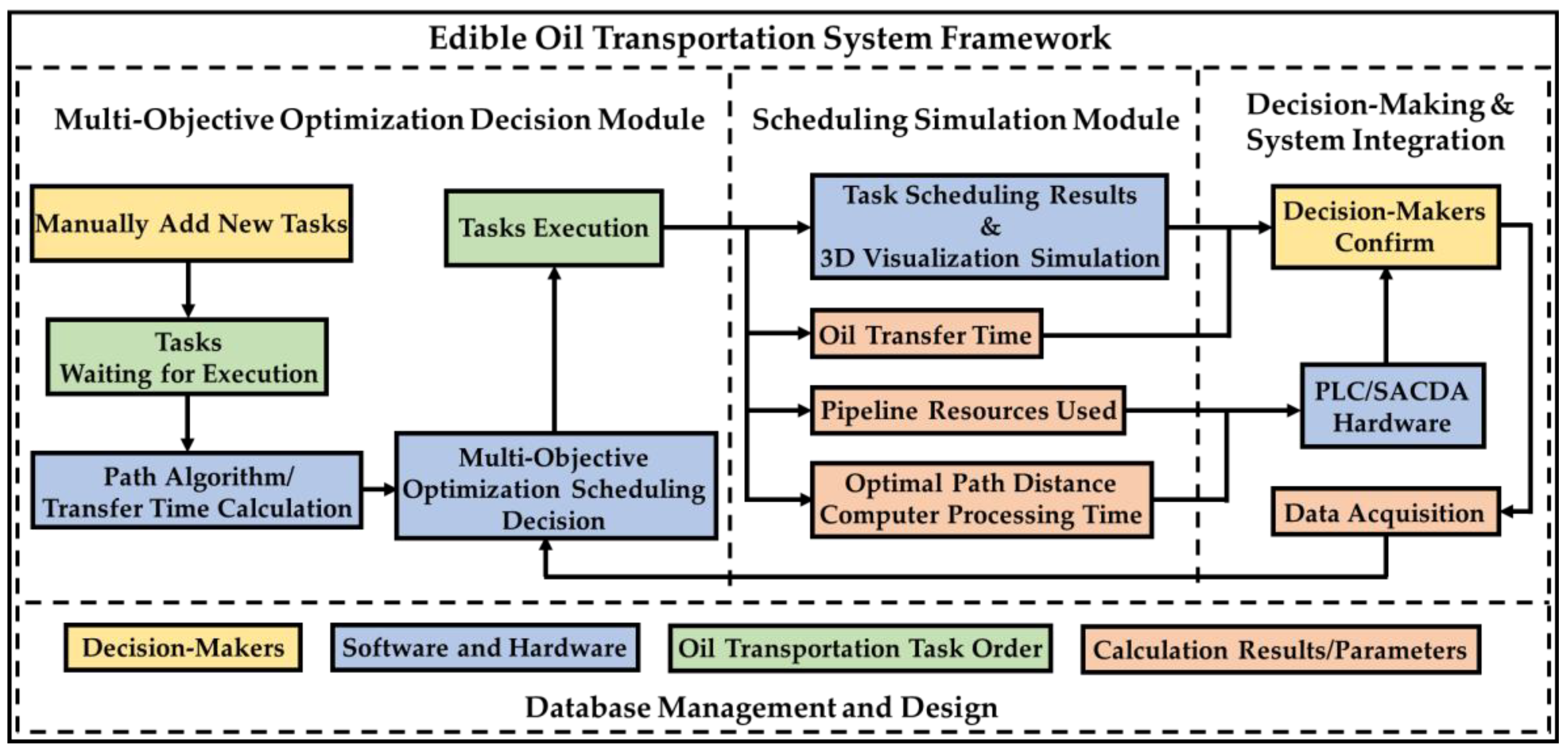


