A Statistical Optimization Method for Sound Speed Profiles Inversion in the South China Sea Based on Acoustic Stability Pre-Clustering

Abstract

Aiming at the problem of accuracy degradation caused by the mixing of spatiotemporal disturbance patterns in sound speed profile (SSP) inversion using the traditional geographic grid division method, this study proposes an acoustic stability pre-clustering framework that integrates principal component analysis and machine learning clustering. Disturbance mode principal component analysis is first used to extract characteristic parameters, and then a machine learning clustering algorithm is adopted to pre-classify SSP samples according to acoustic stability. The SSP inversion experimental results show that: (1) the SSP samples of the South China Sea can be divided into three clusters of disturbance modes with statistically significant differences. (2) The regression inversion method based on cluster attribution reduces the average error of SSP inversion for data from 2018 to 1.24 m/s, which is more than 50% lower than what can be achieved with the traditional method without pre-clustering. (3) Transmission loss prediction verification shows that the proposed method can produce highly accurate sound field calculations in environmental assessment tasks. The acoustic stability pre-clustering technology proposed in this study provides an innovative solution for the statistical modeling of marine environment parameters by effectively decoupling the mixed effect of SSP spatiotemporal disturbance patterns. Its error control level (<1.5 m/s) is 37% higher than that of the single empirical orthogonal function regression method, showing important potential in underwater acoustic applications in complex marine dynamic environments.

1. Introduction

In the field of marine acoustics, the sound speed profile (SSP) is an important waveguide parameter for various underwater acoustic problems, especially in underwater acoustic target recognition, positioning, tracking, and sound field modeling [1]. The general method of obtaining SSPs is on-site real-time measurements, such as direct acquisition through a sound velocity profiler [2], or indirect acquisition through a conductivity–temperature–depth profiler combined with sound speed empirical formulas [3]. The main drawbacks of this method are the huge consumption of human and material resources and the low efficiency caused by point-by-point measurements, which cannot meet the large data needs of marine research.

In recent years, to obtain SSPs more conveniently, the method of inverting SSPs based on environmental parameters has developed rapidly. In 1995, Tolstoy used the matched field processing framework to invert SSPs and achieved good results [4]. Later, Markaki et al. introduced a genetic algorithm into the matched field processing framework to improve the accuracy of SSP inversion further [5]. In 1997, Taroudakis et al. inversed SSPs using matched field processing and a hybrid scheme for vertical slice tomography, achieving high-precision inversion [6]. Although the matched field processing method can effectively solve the problem of data volume demand, it takes a long time to run the method, and the solution to the inverse problem has obvious nonuniqueness.

With the development of machine learning algorithms, neural network models have gradually been introduced into the field of SSP inversion [7]. Huang et al. proposed an SSP inversion model combining an artificial neural network and pre-ray theory, realizing real-time monitoring of shallow sea SSPs [8]. Lu et al. used a hierarchical long short-term memory neural network to construct a prediction model for full ocean depth SSPs, but it depends highly on sonar observation data and focuses on constructing a spatial sound speed field [9]. Machine learning algorithms require a large amount of data, and with the continuous accumulation of data over recent years, data-driven machine learning inversion methods have gradually emerged. Chapman proposed a subsurface SSP inversion method based on self-organizing maps [10]. Su et al. used the extreme gradient boosting algorithm to estimate global subsurface temperature anomalies and salinity anomalies based on satellite observations and Argo data [11]. Ou et al. used a neural network to combine multiple sea surface parameters to enhance the accuracy of SSP inversion [12], providing a more efficient method for SSP inversion. However, although machine learning-based SSP estimation methods have shown good performance in most cases, the estimation accuracy of such data-intensive statistical methods still faces challenges when applied to areas with local disturbances.

The sound speed in seawater can be calculated from the temperature and salinity of seawater. Sea level (SL) data and sea surface temperature (SST) data can be obtained by satellite remote sensing, from which temperature and salinity profiles can be estimated and the SSP of the target sea area can be calculated using empirical formulas. Generally, when estimating SSPs, the empirical orthogonal function (EOF) can be used to reduce the dimensions of unknown parameters. Carnes proved that there is a certain relationship between SL, SST, and EOF [13], and used this relationship to estimate SSPs in the northwest Atlantic Ocean and northwest Pacific Ocean [14]. Later, Chen et al. applied this method to global SSP inversion, effectively confirming the effectiveness of the single empirical orthogonal function regression [15]. The above methods estimate the sound speed profile using linear relationships. However, in the South China Sea, where dynamic characteristics are complex, a single linear relationship cannot effectively explain the connections between dynamic features, sea surface parameters, and the sound speed profile, which in turn leads to a decline in inversion accuracy.

The submarine landform of the South China Sea presents a typical three-layer ring structure, which is formed of a continental shelf–continental slope–central sea basin structure that spans from the periphery to the center, manifesting as a diamond-shaped distribution [16]. This unique submarine landform is completely different from the symmetrical spreading mid-ocean ridge of the Atlantic Ocean or the linear trench–arc system of the Pacific Ocean, reflecting the composite tectonic background of continental margin extension–subduction–collision, with significant mesoscale characteristics, in the South China Sea [17]. The South China Sea has a rare deep water mass active invasion mechanism, whereby deep circulation exchanges water with the Pacific Ocean through a “deep sea waterfall” (water depth of 2500 m) in the Luzon Strait [18,19,20]. The unique geomorphic structure and hydrodynamic characteristics of the South China Sea bring challenges to SSP inversion. At the same time, due to the difficulty of data collection, politics, economics, and other reasons, SSP samples of the South China Sea are scarce, which limits the accuracy of the statistical-based SSP inversion method.

Considering the impact of the unique disturbance characteristics of the South China Sea on statistical methods, which causes errors in sound speed profile estimation, this paper uses South China Sea Argo data and the EOF to extract the main disturbance modes, and carries out cluster analysis on the main disturbance modes to discuss the acoustic stability characteristics of the sea. On the basis of clustering, a regression relationship is established based on Argo profiles and SST and SL data to inverse SSPs. A sound field simulation is conducted to verify the effectiveness of the proposed method in terms of transmission loss, and then the Argo float data from 2018 are used to verify the SSP accuracy.

The main contributions of this paper are as follows:

• Proposed a new method for extracting disturbance features and pre-clustering acoustic stability, which effectively solves the problem of uneven distribution in sample division by traditional grids.
• Based on the random distribution characteristics of the Empirical Orthogonal Function (EOF) in the South China Sea, revealed significant differences in dynamic features among different clustering categories, provided a new perspective for acoustic stability analysis, and further improved the accuracy of sound speed profile inversion in the South China Sea region.
• Through the correlation analysis between statistical clustering and physical mechanisms, clarified the rationality of clustering results as key factors affecting acoustic stability.

The method for extracting disturbance features and acoustic stability pre-clustering is presented in Section 2, also describes the data used in the study; Section 3 and Section 4 respectively present the research results of acoustic stability pre-clustering and the conclusions. Compared with traditional single machine learning methods, this study introduces a disturbance mechanism to further improve the estimation accuracy of sound speed profiles. From the perspective of dynamic characteristics, the sEOF-r method is constrained to solve the problem of low inversion accuracy in local areas. Through the above improvements, the requirements for the accuracy and coverage of sound speed profiles in the actual marine environment perception process can be met.

2. Materials and Methods

2.1. Sound Speed Profile Dimensionality Reduction Method

An SSP is essentially a three-dimensional matrix, where different dimensions of the matrix reflect different distribution characteristics of the SSP. The first dimension of the SSP reflects the vertical distribution characteristics of the sound speed in seawater, and the other two dimensions reflect the spatiotemporal distribution characteristics of the sound speed. Analyzing SSPs in multiple dimensions requires the use of multidimensional variables for machine learning. However, to reduce the complexity of machine learning when fitting SSPs and avoid variables with smaller weights, the sEOF-r method is introduced to perform dimensionality reduction processing on the SSPs. In the SSP inversion problem, the general SSP can be expressed as [21]

$$c\left(z\right)=c_0\left(z\right)+{\sum }_{n=0}^m a_n{\psi }_n\left(z\right),$$

(1)

where z represents the depth distribution characteristics of the SSP; c₀ represents the background profile, that is, the stable and unchanging part of the spatiotemporal sound speed; ψ_n represents the EOF, which is a basis function that changes with time, and its specific mode can be used to describe a certain disturbance form of the SSP; a_n are the EOF projection coefficients, reflecting the weight of each mode disturbance coefficient; and n represents the order of the EOF, reflecting the size and importance ranking of different modes in the data. In the mainstream acoustic inverse problem, due to the existence of noise, a too high EOF order will mistake noise for effective signals. Therefore, the EOF retains the first few orders of modes to obtain a high cumulative variance contribution rate. In the subsequent experiments of this paper, we use an order of 3 to obtain the highest inversion accuracy.

As a typical basis function extraction method, the EOF can extract the main components of an SSP. Usually, an SSP sample is a two-dimensional matrix, W, with dimensions of m × n, where m is the number of discrete depths in each SSP and n is the total number of SSP samples. The irregular matrix, K, is obtained by subtracting the background profile from W, and then the covariance matrix of K is solved as

$$T=K\times K^{\prime }.$$

(2)

The empirical orthogonal matrix is calculated using the covariance matrix, T, and its eigenvalues:

$$T\times s=s\times \lambda .$$

(3)

In the above formula, λ represents the eigenvalue of the covariance matrix T, and s represents the empirical orthogonal matrix, whose dimensions are m × m.

The EOF can be applied to the principal component extraction of SSP disturbance modes. In order to perform SSP inversion effectively, it is necessary to explore the possible connection between the EOF projection coefficients and the SSP to strengthen the inversion accuracy.

2.2. Acoustic Stability Method

According to the regression analysis of a large number of samples, it is confirmed that there is a linear relationship between the sea surface parameters and the EOF projection coefficients [13]. The regression relationship between the sea level anomaly (SLA), sea surface temperature anomaly (SSTA), and the EOF projection coefficients can be expressed as [13]

$$a_n=A_{i,0}+A_{i,1}\times SLA+A_{i,2}\times SSTA+A_{i,3}\times SLA\times SSTA, i=\mathrm{0,1},2\dots n,$$

(4)

where a₀(t) is a constant value and A_i are the coefficients that need to be obtained through regression analysis of a large data set. After obtaining A_i, SLA and SSTA data are input into Equation (4) to calculate the EOF projection coefficients of the corresponding orders. Finally, the SSP is inversed through Equation (1). The inversion accuracy of Equation (1) is related to the consistency of the profile disturbance law. When the profile disturbance laws are consistent, the obtained fitting coefficients are similar, and the final inversion result can achieve high accuracy. The above method demonstrates the importance of acoustic stability factors in SSP inversion.

For the acoustic stability factors, air–sea interactions play a key role. Material and energy exchange in the ocean have a key impact on several important indicators in the sound speed empirical formula. For example, dynamic characteristics of the ocean affect the exchange of salt and energy, thereby directly changing the salt and temperature indicators in the corresponding sea areas. This impact does not have an accurate analytical expression, meaning the specific seawater dynamic characteristics of a certain area cannot be fully described. Therefore, the method of introducing physical constraints to analyze acoustic stability to improve the accuracy of SSP inversion is not applicable. Moreover, there are a large number of random factors in seawater that affect SSP stability. As these dynamic characteristics cannot be calculated using analytical equations, it is necessary to introduce a machine learning algorithm with a high randomness mechanism and a feature selection scheme into the analysis.

2.3. Empirical Orthogonal Function Consistency Analysis of Sound Speed Profiles in the South China Sea Based on K-Means Clustering Analysis

SSPs are widely used in the field of marine acoustics and are the basic support data for various studies. However, due to political, economic, and sampling difficulties, the distribution of Argo floats in the South China Sea is relatively sparse, making it difficult to support machine learning–based studies that require a large amount of data. Current Argo data have great time coverage, but lack spatial coverage, resulting in the overall data being more easily analyzed from the perspective of time, as they cannot meet the needs of regression analysis from the perspective of space. From the perspective of Argo float distribution density, in a 1° × 1° geographic grid spanning 18° N to 19° N and 118° E to 119° E from 2008 to 2018, only 147 SSPs can be queried, and the measurement time period is relatively concentrated. From a statistical point of view, the lack of samples and uneven distribution will increase the instability of the results. Facing the problem of a lack of samples, the primary solution is to expand the SSP inversion area.

The EOF is a completely statistical method, and the physical meaning of each mode order needs to be combined with a relevant dynamic analysis to avoid overfitting the results. Simply expanding the inversion area to which the EOF is fit will be accompanied by a decrease in EOF consistency. The pre-clustering method can effectively divide regions with unique dynamic characteristics. Compared with other clustering algorithms such as hierarchical clustering, K-means is suitable for processing structured data with dense distribution and moderate dimensions, which is consistent with the distribution characteristics of Argo float data in the South China Sea [22]. Therefore, this paper uses the K-means clustering method to carry out cluster analysis on the EOF projection coefficients to analyze the acoustic stability factors and discuss their regional consistency, which allows us to produce more accurate SSP inversion results.

In the process of obtaining the EOF projection coefficients, the high-dimensional original data are compressed into a small number of modes through EOF decomposition, where each SSP sample is represented by low-dimensional projection coefficients. Each EOF mode has a clear physical meaning. For example, the first mode reflects thermal changes in the sea surface, while the second mode reflects salinity effects in the middle layer. Cluster analysis of the EOF projection coefficients can be used to analyze the key factors of acoustic stability. To explore the consistency of the EOF we employed profile data of the South China Sea. After processing, a total of 3881 SSPs were obtained.

Our method is described as follows. First, the background profiles of all data are created, the empirical orthogonal matrix is calculated, the EOF projection coefficients are calculated using SLA and SSTA data, and the SSPs are inversed using the background profiles and projection coefficients, which are also used to analyze the inversion accuracy. Second, a clustering analysis step is added to the above method. After obtaining the background profiles, empirical orthogonal matrix, and EOF projection coefficients, cluster analysis is performed on the EOF projection coefficients. In the case of completed classifications, combined with the EOF projection coefficients of different categories, the corresponding background profiles are used for SSP inversion. Finally, the inversion errors before and after classification are compared to determine the effectiveness of the clustering method for acoustic stability analysis.

When using K-means to carry out cluster analysis of the EOF projection coefficients, the EOF projection coefficients calculated statistically are generally used as the training set, and the i-th order projection coefficient, a_i, of the n-th sample is used to calculate the weight of all samples in the i-th order mode of each cluster [23]:

$$A_i^{\left(k\right)}={\displaystyle \frac{1}{N_k}}\sum _{n=1}^N {\omega }_{kn}{a}_i^{\left(n\right)},$$

(5)

where N_k is the total number of samples in the k-th cluster; A_i(k) represents the mean value of the i-th order EOF projection coefficient in the k-th cluster, that is, the value of the cluster center in the i-th dimension; and ω_kn is the cluster indicator function, which is used to determine whether sample n belongs to the k-th cluster: ω_kn = 1 when n belongs to the k-th cluster and it equals zero when it does not.

After obtaining the value of Ai(k), the Euclidean distance of the cluster is calculated as [23]

$$\epsilon ={\sum }_{n=1}^N{\sum }_{k=1}^K{\omega }_{kn}{\sum }_{i=1}^G{(a_i^{\left(n\right)}-A_i^{\left(k\right)})}^2$$

(6)

where ε is the sum of the squares of the Euclidean distances from all samples to their cluster centers, G is the order of the EOF modes used for inversion, and K is the total number of categories after clustering. ε provides a measure of the compactness of the cluster, where smaller values indicate a better clustering effect.

Figure 1 shows the results of the acoustic stability pre-clustering analysis. Red, blue, and yellow represent three different clustering results. The clustering results have no specific physical basis and are completely statistically-based. They may be related to seasons and disturbance modes, but the clustering results are all key factors affecting acoustic stability. However, compared with the traditional method of dividing samples by grids, the Empirical Orthogonal Function (EOF) of the South China Sea presents random distribution characteristics, with differences in acoustic stability, and each category has distinct dynamic features. After the cluster analysis is completed, each cluster center is used as a background profile for the corresponding sea surface parameter samples.

The core of acoustic stability clustering research is to combine the stability characteristics of sea surface parameters with the disturbance characteristics of SSPs for comprehensive cluster analysis, which requires large samples of SSP, SLA, and SSTA data. After carrying out the EOF analysis on an SSP, the EOF covariance matrix is obtained, and the SSP can be inversed using the covariance matrix and the EOF projection coefficients fitted via the SLA and SSTA data. Therefore, the two most important data sources in the actual inversion process are SSP and sea surface data. Obtaining the above two types of data for the target sea area can complete the work of expanding the inversion area.

2.4. Sound Speed Profile Data

The main way to obtain SSP samples of the South China Sea currently is through Argo float data. The Argo program began in 1999, which, from 2007, formed an observation network composed of 3000 floats, each with the ability to collect ocean temperature–salinity profiles, providing a basis for the calculation of SSPs. As of 2020, the number of Argo floats increased to nearly 4000, and the coverage has expanded to high latitudes, marginal seas, and deep-sea areas.

The submarine structure of the South China Sea is complex, with widely distributed continental shelves and slopes. The central sea basin is a typical oceanic crust expansion area, with a water depth of more than 4000 m. At the same time, there are many groups of seamount chains and fracture zones, which affect the distribution of seawater chemical properties and heat flux in some areas. The South China Sea also has complex seawater dynamic characteristics. The monsoon-driven surface circulation system affects the temperature and salinity distributions. Moreover, mesoscale eddies significantly change the local temperature–salinity structure through vertical shear and horizontal convergence–divergence. In general, the submarine landform structure and complex hydrodynamic characteristics of the South China Sea have a significant impact on acoustic stability.

Combining the special geomorphic characteristics and seawater dynamic characteristics of the South China Sea with the Argo float data, we selected data spanning 12° N to 20° N and 110° E to 120° E from 2009 to 2017 as the training sample for the EOF. Since the number of Argo float samples decreases sharply when the depth exceeds 1000 m, and several factors adversely affecting acoustic stability mainly exist at depths exceeding 1000 m, the research depth studied in this paper is 0–1000 m. Considering the common profile depth intervals used in oceanographic research, adopting a recognized sampling interval is conducive to comparison with other methods. Referring to the World Ocean Atlas (2023; WOA) standard, linear interpolation was performed on the 0–1000 m depth data with a basic sampling interval of 5 m. After the above processing, a total of 3881 SSPs were obtained, of which 3758 were used for training and 123 were used for verification after SSP inversion.

In the process of carrying out EOF analysis of the SSPs, the temperature–salinity profile WOA data from 2005–2008 were used to calculate annually averaged SSPs. The SSP calculation method was the same as that used for the Argo data, and the SSPs were calculated using the sound speed empirical formula with the temperature and salinity profiles as variables.

2.5. Sea Surface Data

The SST and sea surface height are key parameters used for SSP inversion, with both accessible from marine remote sensing data. The data used here come from the Copernicus Program, which is a global Earth observation and environmental monitoring program led by the European Union (https://marine.copernicus.eu/). The sea surface height data employed in this study come from the altimeter satellite of the Copernicus Program. The absolute sea surface height is inverted by accurately measuring the distance between the satellite and the sea surface through a radar altimeter, combined with an Earth gravity field model and the satellite’s orbital parameters. The SLA data used here are integrated with the above multiple altimeter satellite data sets. After preprocessing using the optimal interpolation method, the final spatial resolution is 0.25°. The SST data used here come from the Global High-Resolution Project, which captures short-term changes in the SST and have a spatial resolution of 0.05°. The two sets of remote sensing data, SLA and SSTA, have daily temporal resolution. After obtaining the two types of remote sensing data, it is necessary to match the remote sensing data with the Argo float data. In the matching process, the nearest neighbor rule is adopted to match the remote sensing data with the nearest Argo float data spatially.

3. Results

The key point of the acoustic stability clustering method is the number of categories after sample clustering. The contribution of acoustic stability factors to the statistical optimization of the SSP is studied by using the influence of the number of categories on the inversion accuracy of the SSP. To obtain the results, a sample cluster analysis is first carried out; the inversion errors of the SSP are determined by considering the one-category (i.e., unclustered) and three-category clustering results; and then the data are analyzed from the perspective of how the accuracy changes as a function of sample size and time. After completing the classification, by considering the role of seasonal circulation, the inversion effects of the one-category and three-category clustering results in each of the four seasons are analyzed.

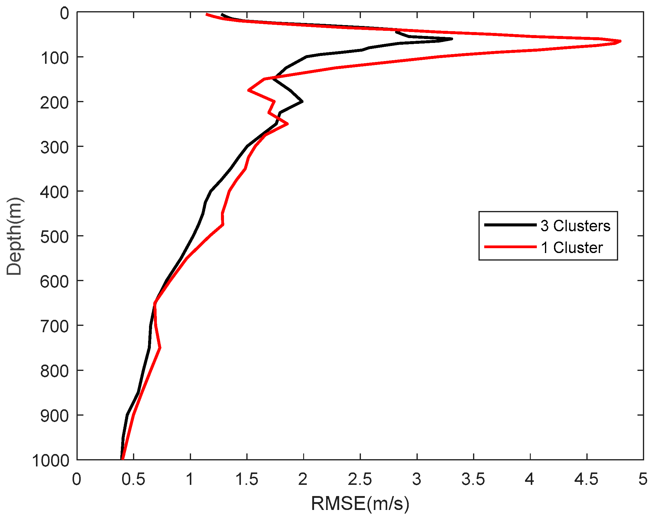
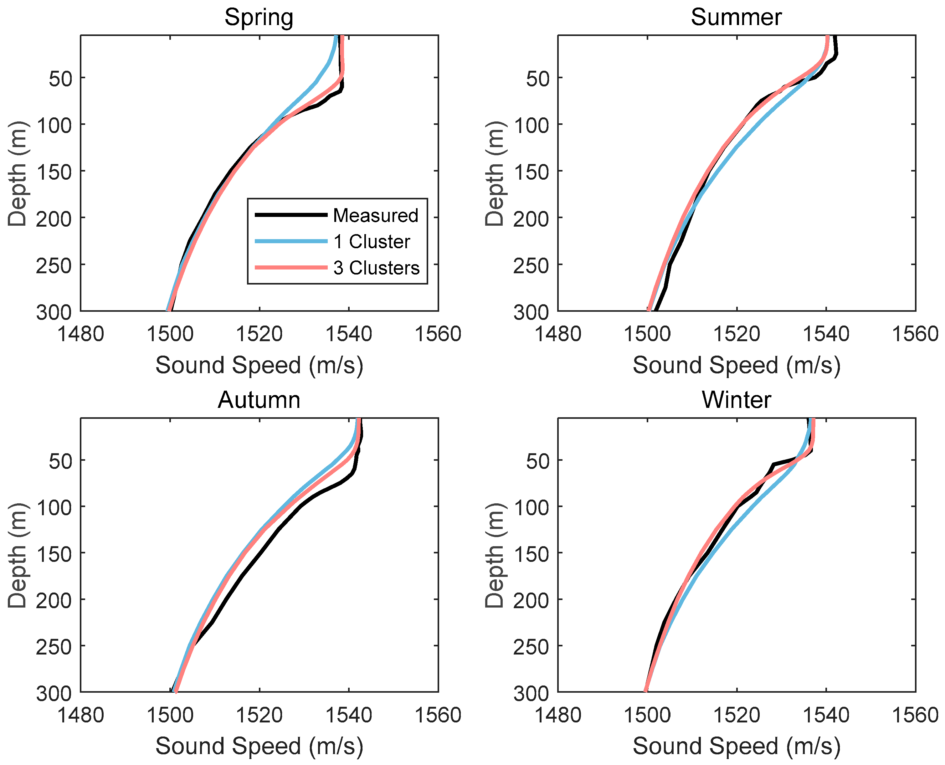
3.1. Inversion Effect of Sound Speed Profiles After Clustering

The root mean square error (RMSE), quantified as the difference between direct inversion without clustering and inversion after three-category clustering, is shown in Figure 2. It can be seen from the figure that the accuracy after acoustic stability clustering is significantly higher than before clustering at most depths. The average RMSE obtained after acoustic stability clustering is 1.67 m/s, while the average RMSE obtained by direct inversion is 2.03 m/s. Compared with the method of directly using the s-EOF-r for inversion, the acoustic stability pre-clustering method extracts the main types of disturbances, significantly reducing the RMSE at sea depths of 0–150 m; however, the improvement effect is relatively limited at water depths below 150 m, among which the RMSE after clustering in the region of 150–250 m shows a significant rebound. This phenomenon is because the sound speed characteristics in this layer are relatively stable, and the performance of the pre-clustering method will decrease when facing such sudden changes in acoustic stability. The maximum RMSE of the s-EOF-r inversion method at sea depths of 0–150 m reaches 4.79 m/s, and after pre-clustering, it is reduced to 3.30 m/s. Two peaks in the inversion error appear at 60 m and 200 m, which come from random, large gradient disturbances at these depths. Generally, the randomness of this kind of disturbance is difficult to explain using traditional physical analysis methods, resulting in certain challenges for the physical mechanism method of sEOF-r in solving related problems.

Figure 3 shows the RMSE as a function of sample’s serial number, the RMSE value of each sample point represents the average RMSE of all inversion results within a sea depth of 1000 m at that point. It can be seen that the RMSE after acoustic stability clustering is generally better than before clustering. The RMSE before clustering fluctuates around 3 m/s, including two prominent peaks at 5.22 m/s and 5.00 m/s. The RMSE of the SSP after acoustic stability clustering is generally below 2.5 m/s, and the maximum RMSE does not exceed 4 m/s. The extraction and classification of sample features by acoustic stability pre-clustering enable the sEOF-r to separate the main modes of sea surface disturbance more efficiently, further reducing the error in subsequent inversion.

From the perspective of the mean value of the SSP inversion error, the accuracy of the acoustic stability pre-clustering method is slightly higher than that of the non-clustering method. From Figure 3, it can be seen that the RMSE peaks of the two methods basically match, indicating that the main components interfering with the inversion process are consistent. In terms of the maximum inversion error, the RMSE of the acoustic stability clustering method is significantly lower than that of the non-clustering method, while at the place where the errors of both are low, this performance is not obvious. The main source of the error peak is the change of the water body structure caused by seasonal circulation in the South China Sea, which has a significant impact on the SST and sea surface height.

To study the impact of the seasonal characteristics of the sea surface parameters in the South China Sea on the acoustic stability clustering method further, Figure 4 shows the typical inversion effects of the SSP in each of the four seasons. Compared with the non-clustering method, the acoustic stability clustering method has significant advantages for the spring and winter data. Although the acoustic stability clustering method is based on statistical principles, making it generally difficult to explain the occurrence of random water masses and fronts from a physical perspective, it can still effectively reflect disturbances near the sea surface. For the SSP inversion results for data at greater depths, from the winter results, two abnormal values appear in the SSP at 50 m and 100 m, and the acoustic stability pre-clustering method fails to show this abnormal disturbance.

SSP inversion requires establishing a connection between the sea surface parameters and the background profile. Although the background profile cannot reflect abnormal disturbances at a specific time, the sea surface parameters can effectively reflect shallow abnormal disturbances under the premise of pre-clustering. Although the pre-clustering method has certain errors in solving deep disturbances, as seen in the inversion effects for the four seasons shown in Figure 4, the inversed profiles are basically consistent with the measured profiles, and they are more accurate than those obtained with the non-clustering method.

3.2. Transmission Loss Simulation

In underwater acoustic problems, SSPs are mainly used for sound field simulation, where the inversion accuracy of the former determines the accuracy of the latter. Thus, sound field simulation results can directly verify whether the inversed SSPs are effective.

Figure 5 shows the transmission loss results from the sound field simulations using the inversed profiles combined with the Krakenc model. The SSP inversion depth is 1000 m. Considering that the inversion errors tend to be stable when the inversion depth is greater than 600 m, inversed profiles with depths of 1000 m were extrapolated to 4000 m in the experiment to reflect the sound field structure more completely. In the sound field simulation, the sound source depth is 100 m, the receiver depth is 50 m, the sound source frequency is 100 Hz, the seabed density is 1.73 g/cm³, and the seabed sound speed is 1541 m/s.

The transmission loss results show that both methods have large errors at 3.5 km, of about 10 dB, which are caused by abnormal disturbances within the inversed profiles. In terms of the transmission loss results within 25 km, both methods basically match the results obtained from the real profile and reflect the sound field structure of the first 10 convergence zones. In the 11th convergence zone from 25 km to 40 km, the non-clustering method begins to show obvious simulation errors, of about 3 dB. These are caused by the sound field simulation errors, which in turn arise from the SSP inversion errors, which accumulate with distance. The method after acoustic stability clustering produces results that are close to the original transmission loss simulation results for depths exceeding 25 km, with an error of about 0.2 dB, reflecting the high consistency between the inversed profile and the original profile.

4. Conclusions

This study has carried out an acoustic stability pre-clustering analysis of EOF projection coefficients, classified the main disturbance types of SSPs in the South China Sea, and used different categories of background profiles according to the clustering results during inversion to improve inversion accuracy. We have shown that Equation (4) confirms that sea surface parameters can be used for SSP inversion, where the EOF projection coefficients play a key role in the inversion process.

An SSP inversion experiment was carried out using data obtained for the South China Sea area, and the results after acoustic stability pre-clustering were compared with the inversion effect of the non-clustering method to verify the improvement of the acoustic stability analysis method on the inversion accuracy of SSPs. The inversion accuracy shows seasonal fluctuations. Compared with the direct inversion method, although the acoustic stability analysis also has seasonal errors, it can effectively reduce this error compared with the direct inversion method. Therefore, introducing the acoustic stability clustering method in the preprocessing of SSPs can significantly improve the efficiency of SSP inversion. Some samples within the study range have strongly random disturbances, which are the main reasons for the SSP inversion errors. While the method of directly using EOF inversion cannot clearly express these random disturbances, the pre-clustering method is able to account for them. After carrying out an acoustic stability pre-clustering analysis of the disturbances, the inversion errors were reduced by about 20% compared with direct inversion, producing profiles that are basically consistent with the true SSPs. Although both the acoustic stability analysis method and the direct inversion method have obvious errors near the sea surface, the lower inversion errors of the acoustic stability analysis method provide the possibility for obtaining SSPs worldwide. The highly accurate inversion results mean that high-resolution and high-precision SSPs can be obtained for areas all across the globe directly through remote sensing data without field measurements.

Finally, through the transmission loss simulation experiment, it was concluded that the inversed SSPs can be used for a wide range of experiments, such as sound field calculation. Sound field simulation is the basis for applications such as sonar performance evaluation and matched field inversion. By using the acoustic stability analysis method to coordinate remote sensing parameters, the results can be extended to various marine parameters. However, in the subsurface depth of seawater, the performance of the pre-clustering method is affected by the sudden changes in acoustic stability. This issue needs to be addressed by further constraining the stability conditions in future work.

References

1. Porter, M.B.; Bucker, H.P. Gaussian beam tracing for computing ocean acoustic fields. J. Acoust. Soc. Am. 1987, 82, 1349–1359. [Google Scholar] [CrossRef]
2. Zhang, S.; Xu, X.; Xu, D.; Long, K.; Shen, C.; Tian, C. The design and calibration of a low-cost underwater sound velocity profiler. Front. Mar. Sci. 2022, 9, 996299. [Google Scholar] [CrossRef]
3. GmbH, S.S.T. Sea & Sun Technology CTD Probes. 2023. Available online: https://www.sea-sun-tech.com/ (accessed on 1 June 2024).
4. Tolstoy, A.; Diachok, O.; Frazer, L. Acoustic tomography via matched field processing. J. Acoust. Soc. Am. 1991, 89, 1119–1127. [Google Scholar] [CrossRef]
5. Taroudakis, M.I.; Markaki, M.G. Matched field ocean acoustic tomography using genetic algorithms. In Acoustical Imaging; Springer: Berlin/Heidelberg, Germany, 1995; pp. 601–606. [Google Scholar] [CrossRef]
6. Taroudakis, M.I. On the use of matched-field processing and hybrid algorithms for vertical slice tomography. J. Acoust. Soc. Am. 1997, 102, 885. [Google Scholar] [CrossRef]
7. Stephan, Y.; Thiria, S.; Badran, F. Inverting tomographic data with neural nets. In Proceedings of the ‘Challenges of Our Changing Global Environment’. Conference Proceedings. OCEANS ‘95 MTS/IEEE, San Diego, CA, USA, 9–12 October 1995. [Google Scholar] [CrossRef]
8. Huang, W.; Li, D.; Jiang, P. Underwater sound speed inversion by joint artificial neural network and ray theory. In The Thirteenth ACM International Conference; ACM: New York, NY, USA, 2018. [Google Scholar] [CrossRef]
9. Lu, J.; Zhang, H.; Wu, P.; Li, S.; Huang, W. Predictive modeling of future full-ocean depth SSPs utilizing hierarchical long short-term memory neural networks. J. Mar. Sci. Eng. 2024, 12, 943. [Google Scholar] [CrossRef]
10. Chapman, C.; Charantonis, A.A. Reconstruction of Subsurface Velocities From Satellite Observations Using Iterative Self-Organizing Maps. Geosci. Remote Sens. Lett. 2017, 14, 617–620. [Google Scholar] [CrossRef]
11. Su, H.; Yang, X.; Lu, W.; Yan, X.-H. Estimating subsurface thermohaline structure of the global ocean using surface remote sensing observations. Remote Sens. 2019, 11, 1598. [Google Scholar] [CrossRef]
12. Ou, Z.; Qu, K.; Wang, Y.; Zhou, J. Estimating sound speed profile by combining satellite data with in situ sea surface observations. Electronics 2022, 11, 3271. [Google Scholar] [CrossRef]
13. Carnes, M.R.; Mitchell, J.L.; de Witt, P.W. Synthetic temperature profiles derived from Geosat altimetry: Comparison with air-dropped expendable bathythermograph profiles. J. Geophys. Res. Ocean. 1990, 95, 17979–17992. [Google Scholar] [CrossRef]
14. Carnes, M.R.; Teague, W.J.; Mitchell, J.L. Inference of Subsurface Thermohaline Structure from Fields Measurable by Satellite. J. Atmos. Ocean. Technol. 1994, 11, 551–566. [Google Scholar] [CrossRef]
15. Chen, C.; Ma, Y.; Liu, Y. Reconstructing Sound Speed Profiles Worldwide with Sea Surface Data. Appl. Ocean Res. 2018, 77, 26–33. [Google Scholar] [CrossRef]
16. Li, W.; Alves, T.M.; Wu, S.; Völker, D.; Zhao, F.; Mi, L.; Kopf, A. Recurrent slope failure and submarine channel incision as key factors controlling reservoir potential in the South China Sea (Qiongdongnan Basin, South Hainan Island). Mar. Pet. Geol. 2015, 64, 17–30. [Google Scholar] [CrossRef]
17. Weller, M.D. Subtidal Variability in the Northern South China Sea during Spring 2001. Master’s Thesis, Naval Postgraduate School, Monterey, CA, USA, 2005. [Google Scholar]
18. Yuan, D.L. A numerical study of the South China Sea deep circulation and its relation to the Luzon Strait transport. Acta Oceanol. Sin. 2002, 21, 187–202. [Google Scholar]
19. Wang, D.; Wang, Q.; Cai, S.; Shang, X.; Peng, S.; Shu, Y.; Xiao, J.; Xie, X.; Zhang, Z.; Liu, Z.; et al. Advances in research of the mid-deep South China Sea circulation. Sci. China Earth Sci. 2019, 62, 1992–2004. [Google Scholar] [CrossRef]
20. Mai, H.; Wang, D.; Chen, H.; Qiu, C.; Xu, H.; Shang, X.; Zhang, W. Mid-Deep Circulation in the Western South China Sea and the Impacts of the Central Depression Belt and Complex Topography. J. Mar. Sci. Eng. 2024, 12, 700. [Google Scholar] [CrossRef]
21. Michael, B.; Peter, G. Dictionary learning of sound speed profiles. J. Acoust. Soc. Am. 2017, 141, 1749–1758. [Google Scholar] [CrossRef]
22. Shudong, H.; Zhao, K.; Zenglin, X.; Liu, Q. Robust Deep K-Means: An Effective and Simple Method for Data Clustering. Pattern Recognit. 2021, 117, 107996. [Google Scholar] [CrossRef]
23. Ou, Z.; Qu, K. Research on sound speed profile estimation method in the South China Sea based on K-means clustering analysis and single empirical orthogonal function regression. Tech. Acoust. 2022, 41, 821–826. [Google Scholar] [CrossRef]
Figure 1. Distribution of the training samples. Red represents the cluster 1, blue represents the cluster 2 and yellow represents the cluster 3.
Applsci 15 08451 g001
Figure 2. RMSE with depth for the one-category (i.e., unclustered) and three-category clustering results.
Applsci 15 08451 g002
Figure 3. RMSE as a function of sample size for the one-category and three-category clustering results.
Applsci 15 08451 g003
Figure 4. Inversion effect in different seasons of the two methods (unclustered vs. clustered).
Applsci 15 08451 g004
Figure 5. Comparing simulated losses from the clustered (red) and unclustered (green) simulations with measured losses (grey).
Applsci 15 08451 g005
Disclaimer/Publisher’s Note: The statements, opinions and data contained in all publications are solely those of the individual author(s) and contributor(s) and not of MDPI and/or the editor(s). MDPI and/or the editor(s) disclaim responsibility for any injury to people or property resulting from any ideas, methods, instructions or products referred to in the content.