Three-Dimensional Numerical Study on Fracturing Monitoring Using Controlled-Source Electromagnetic Method with Borehole Casing

Abstract

Hydraulic fracturing is a crucial technology for developing unconventional oil and gas resources. However, conventional geophysical methods struggle to efficiently and accurately image proppant-connected channels created by hydraulic fracturing. The borehole-to-surface electromagnetic imaging method (BSEM) overcomes this limitation by utilizing a controlled cased well source. Placing the source close to the target reservoir and deploying multi-component receivers on the surface enable high-precision lateral monitoring, providing an effective approach for dynamic monitoring of hydraulic fracturing operations. This study focuses on key aspects of forward modeling for BSEM. A three-dimensional finite-volume method based on the Yee grid was used to simulate the borehole-to-surface electromagnetic system incorporating metal casings, validating the method of simulating metal casing using multiple line sources. The simulation of the observation system and the frequency-domain electromagnetic monitoring simulation based on actual well data confirm BSEM’s high sensitivity for monitoring deep subsurface formations. Critically, well casing exerts a substantial influence on surface electromagnetic responses, while the electromagnetic contribution from line sources emulating perforation zones necessitates explicit incorporation within data processing workflows.

1. Introduction

The continuous advancement of geophysical exploration technologies has established borehole hydrocarbon reservoir monitoring as a critical frontier in contemporary geophysical detection [1,2,3]. Conventional surface methods exhibit limitations in evaluating deep subsurface formations, presenting significant challenges including substantial burial depths of monitoring targets, geological complexity of borehole environments, interference sources, and insufficient resolution for target-scale characterization. These challenges necessitate high-precision, high-resolution monitoring solutions [4,5,6,7]. The borehole-to-surface electromagnetic imaging method (BSEM) addresses this need as a geophysical electromagnetic monitoring technology that overcomes traditional surface electromagnetic depth limitations [8,9,10]. By directly establishing the source in target formations through well casings, this electrical excitation source enhances the current density distribution in deep reservoirs, showcasing application potential for dynamic subsurface monitoring [11,12,13]. This method is mainly applied in fine exploration of deep metal mines and hydraulic fracturing monitoring in horizontal wells, with promising application prospects in resource exploration and engineering geological survey fields in the future [14,15,16,17,18,19,20,21,22,23,24,25].

This study focuses on research into frequency-domain electromagnetic monitoring using the BSEM method (Figure 1), which is divided into two excitation modes [26]. One is using the metal casing of a well for excitation, that is, to inject low-frequency alternating current into metal casing well A and connect the negative pole B to another metal casing or ground it at infinity; alternatively, the positive and negative poles of the source can be simultaneously connected to two positions at different depths of the same metal casing (i.e., a vertical bipole source) and then receive the electromagnetic response signals on the surface. The other is placing an electric dipole (point or line) or a magnetic dipole in an open-hole well or a cased well, and receive the electric and magnetic fields on the surface. If the receiving electrodes are placed in another open-hole well, it becomes a crosswell electromagnetic observation method. Therefore, for simulation of the borehole-to-surface electromagnetic method, electromagnetic field simulation theory of dipole sources and line sources is of great significance. The simulation of the BSEM method is implemented via the finite volume method (FVM) [3,7,27].

1.1. Principles of the Finite Volume Method

The finite volume method (FVM) divides the computational domain into a series of non-overlapping control volume elements. By integrating the differential equations to be solved within each control volume, a set of discrete equations is derived. A key feature of the discrete equations obtained by FVM is that the integral conservation of dependent variables must be satisfied for any set of control volumes [7,27]. In contrast, the finite difference method (FDM) only satisfies integral conservation when the grid is extremely fine. FVM can ensure integral conservation even with coarse grids, allowing for more flexible grid division [28,29,30,31,32,33]. In FVM, staggered grid discretization (Yee grid) is commonly used [27].

The Yee grid is a widely adopted grid division method in electromagnetic field simulations and represents a finite-volume extension of tensor-product Cartesian grids with variable grid spacing. In this grid, the spatial sampling points of electric and magnetic field components are staggered such that each electric field component is surrounded by four magnetic field components, and each magnetic field component is surrounded by four electric field components. This arrangement makes the discretization of electromagnetic fields more consistent with physical laws, thus being widely applied in electromagnetic field simulations. The Yee grid facilitates divergence calculations and better simulates characteristics such as electromagnetic wave propagation and scattering [27]. Extensive research has been conducted on its applications in finite difference methods, and further optimization can enable efficient computations in borehole-to-surface electromagnetic imaging scenarios [33,34,35].

1.2. Metal Casings in Borehole-to-Surface Electromagnetic Imaging

In electromagnetic excitation environments involving wells, the presence of metal casings is a complex factor affecting electromagnetic response observations [36,37,38,39]. During crosswell or borehole-to-surface electromagnetic monitoring, metal casings may cause signal attenuation [40,41,42,43]. Additionally, electromagnetic responses from metal casings can generate interference signals that must be considered in numerical simulations or inversions [44,45]. Although metal casings complicate numerical modeling and inversion, they can be regarded as “extended electrodes” that help excite deep targets and enhance signals, which might be unobservable without casings.

Many scholars have discussed solutions for simulating borehole-to-surface electromagnetic imaging observation systems in models with metal casings [46,47,48]. Heagy et al. (2017) verified the effectiveness of borehole-to-surface DC resistivity observations through finite volume simulations [46]. In subsequent research, Heagy et al. (2023) performed finite volume simulations for time-domain and frequency-domain borehole-to-surface electromagnetic methods, demonstrating that magnetic permeability enhances the inductive components of electromagnetic responses [47]. However, the finite volume simulation methods applied to borehole-to-surface electrical exploration techniques still demand further technological advancement and systematic summarization. This is essential to enable them to effectively tackle more intricate geological scenarios and multi-source interference environments, thereby enhancing the accuracy and applicability of electrical method interpretations in complex hydrogeological, engineering geological, petroleum, and mineral exploration projects [49,50,51,52,53,54,55,56,57,58,59,60,61].

For borehole-to-surface electromagnetic imaging technology, it is essential to account for the influence of metal casings and develop efficient simulation methods. The goal is to model the geometry and physical properties of metal casings without compromising computational efficiency or the accuracy of target area calculations, thereby improving the inversion accuracy in target regions.

2. Forward Modeling Method

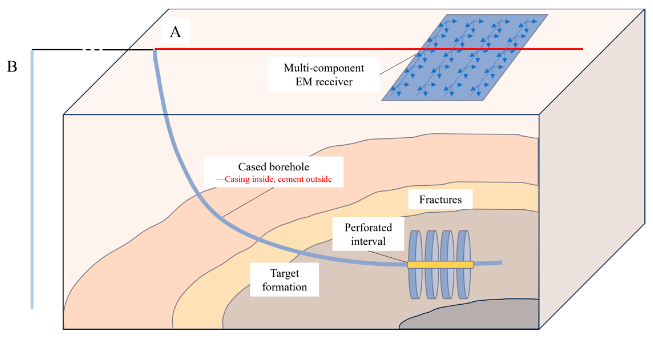
2.1. Borehole-to-Surface Electromagnetic Monitoring System

The borehole-to-surface electromagnetic method (BSEM) (frequency domain) primarily achieves power supply through the metal casing of the target well, transmitting low-frequency pulse signals (square waves or sine waves) into the well and conducting multi-component observations of electromagnetic responses via surface survey networks. Changes in the frequency-domain BSEM field responses observed on the surface reflect alterations caused by borehole hydraulic fracturing operations. Through inversion calculations, three-dimensional imaging of fracture anomalies induced by fracturing is performed to evaluate fracturing effectiveness. The observation system for the frequency-domain borehole-to-surface electromagnetic method is illustrated in Figure 2. During observations, multi-frequency signal transmissions are typically produced, and two electric field components (Ex, Ey) and three magnetic field components (Hx, Hy, Hz) are received on the surface, which yield better monitoring results for application scenarios such as fracturing fracture imaging. This study focuses on discussing the lateral dynamic changes of fracturing, thus primarily addressing Ex, Ey, Hx, and Hy.

The positive pole (A) is connected to the wellhead, while the negative pole (B) is positioned on the surface or connected to another well, typically 2–3 km away from the wellhead. The red line in Figure 2 represents a cased well, which is often simplified as a line source in simulations, decomposed into vertical and horizontal line-source components. The surface survey network is usually deployed along the ground-projected plane of the wellbore trajectory, typically configured as a square grid covering the target fracturing interval to be monitored.

2.2. Underground Electromagnetic Field Simulation Theory

The borehole-to-surface electromagnetic method (frequency domain) is analogous to the frequency-domain controlled-source electromagnetic method (CSEM). According to Faraday’s law and Ampère’s law, the electromagnetic fields in CSEM are governed by the quasi-static Maxwell equations, with displacement currents neglected [3,7]. The quasi-static Maxwell equations are expressed as

$$\nabla \times \mathit{E}=-i\omega \mu \mathit{H},$$

(1)

$$\nabla \times \mathit{H}=\sigma \mathit{E}+{\mathit{J}}_{\mathit{s}},$$

(2)

$$\nabla \cdot \mathit{H}=0,$$

(3)

$$\nabla \cdot \mathit{E}=0,$$

(4)

where $\mathit{E}$ is the electric field strength, with unit $\mathrm{V}/\mathrm{m}$; $\mathit{H}$ is the magnetic field strength, with unit $\mathrm{A}/\mathrm{m}$; $\omega$ is the angular frequency, with unit $\mathrm{rad}/\mathrm{s}$; ${\mathit{J}}_{\mathit{s}}$ is the current density of the externally applied field source, with unit $\mathrm{A}/{\mathrm{m}}^2$; $\mu$ is the magnetic permeability, which can be expressed as $\mu ={\mu }_r{\mu }_0$, where ${\mu }_r$ is the relative magnetic permeability and ${\mu }_0$ is the magnetic permeability of free space; $\sigma$ is the electrical conductivity, with unit $\mathrm{S}/\mathrm{m}$.

Since the magnetic flux density $\mathit{B}=\mu \mathit{H}$, Equations (1) and (2) can also be written as

$$\nabla \times \mathit{E}=-i\omega \mathit{B},$$

(5)

$$\nabla \times {{\mu }_0}^{-1}\mathit{B}={\mathit{J}}_{\mathrm{c}}+{\mathit{J}}_{\mathit{s}},$$

(6)

In Equations (5) and (6), the unit of the magnetic flux density $\mathit{B}$ is $T$. In Equation (6), the conductive current ${\mathit{J}}_{\mathrm{c}}$ obeys Ohm’s law:

$${\mathit{J}}_{\mathbf{c}}=\sigma \mathit{E},$$

(7)

Eliminating the magnetic flux density $\mathit{B}$ from Equations (5) and (6) yields a second-order vector Helmholtz equation for the electric field $\mathit{E}$:

$$\nabla \times {{\mu }_0}^{-1}\nabla \times \mathit{E}+i\omega \sigma \mathit{E}=-i\omega {\mathit{J}}_s,$$

(8)

The magnetic field $\mathit{H}$ can be calculated using the following system of equations:

$$\mathit{H}=-{\displaystyle \frac{1}{i\omega {\mu }_0}}\nabla \times \mathit{E} ,$$

(9)

Considering the low-frequency emission characteristics, the boundary conditions of the entire system are ideal conductor boundaries: $\mathit{n}\times \mathit{E}=0$, $\mathit{n}\cdot \mathit{H}=0$, where $\mathit{n}$ is the outward unit normal vector of the computational domain boundary.

Equation (8) can also be written as

$$\nabla \times \nabla \times \mathit{E}+i\omega {\mu }_0\sigma \mathit{E}=-i\omega {\mu }_0{\mathit{J}}_s.$$

(10)

2.3. Solving the Discretization of the Target Region

To solve Maxwell’s equations numerically, the modeling domain is discretized in a three-dimensional Cartesian coordinate system using hexahedral grids (Yee cells) with variable intervals [27]. The Yee cell discretization places electric fields at the midpoints of grid cell edges and magnetic fields on grid cell faces (Figure 3a), defining conductivity and magnetic permeability at the center of each cell. This discretization method ensures that the tangential component of the electric field is continuous along each edge of the grid cell, and the normal component of the field is continuous across each face of the grid cell. The curl operator can be approximated by integration using the finite volume method. In four adjacent cells, the magnetic field $\mathit{H}$ defined at the face center is surrounded by the electric field $\mathit{E}$ defined at the edge center (Figure 3b). Using Equation (7) and Stokes’s theorem, the weak solution forms of Equations (1) and (2) can be obtained:

$${\displaystyle {\oint }_{\mathrm{\Gamma }}\mathit{E}}\cdot d\mathbf{\Gamma }=-\mathrm{i}\omega {\displaystyle {\iint }_S\mathit{B}}\cdot d\mathit{S},$$

(11)

$${\displaystyle {\oint }_{\mathrm{\Gamma }}\mathit{H}}\cdot d\mathbf{\Gamma }={\displaystyle {\iint }_S\nabla }\times \mathit{H}\cdot d\mathit{S}={\displaystyle {\iint }_S\left(\sigma \mathit{E}+{\mathit{J}}_s\right)}\cdot d\mathit{S},$$

(12)

where $\mathit{S}$ denotes the cross-sectional area of the control volume in the XOZ plane. By using the first equation in (12), the curl operator can be approximated as the line integral of the field along a closed path normalized by the area $\mathit{S}$. It can be seen from the second equation in (12) that the line integral of $\mathit{H}$ along the closed loop is equal to the surface integral of the current density within the loop [7,27]. Assuming that the electric field in the Y-direction within the control volume is uniform, similar to a parallel circuit, the total current density in the Y-direction excluding external sources is equal to the sum of the surrounding four cells:

$${\displaystyle {\iint }_S\overline{\sigma }}\mathit{E}\cdot d\mathit{S}={\displaystyle \sum _{i=1}^4{\displaystyle {\iint }_{S_i}{\sigma }_i}}\mathit{E}\cdot d{\mathit{S}}_i,$$

(13)

where $\overline{\sigma }$ is the average electrical conductivity, ${\sigma }_i$ is the electrical conductivity in the i-th cell, and ${\mathit{S}}_i$ is the cross-sectional area of the i-th cell.

From Equation (13), the average electrical conductivity defined on the grid edge can be calculated as the area-weighted average of the adjacent four conductivities:

$$\overline{\sigma }={\displaystyle \sum _{i=1}^4\frac{S_i}{S}}{\sigma }_i,$$

(14)

The average conductivity $\overline{\sigma }$ in Equation (14) can be computed using the averaging matrix $\mathit{A}$. The averaging matrix ${\mathit{A}}_{E2C}$ maps variables from the midpoints of grid cell edges to the centers of cell volumes. Another averaging matrix ${\mathit{A}}_{F2C}$ for staggered grids maps variables from the centers of cell faces to the centers of cell volumes. The matrix forms of Equations (11) and (12) are

$${{\mathit{Cell}}_F}^{\mathrm{T}}\mathrm{diag}\left[{\mathit{A}}_{F2C}^{\mathrm{T}}\mathit{v}\right]\mathit{C}\mathit{E}=-i\omega {{\mathit{Cell}}_F}^{\mathrm{T}}\mathrm{diag}\left[{\mathit{A}}_{F2C}^{\mathrm{T}}\mathit{v}\right]\mathit{B},$$

(15)

$${{\mathit{Cell}}_E}^{\mathrm{T}}\mathit{C}\mathrm{diag} \left[{\mathit{A}}_{F2C}^{\mathrm{T}}\left({\mu }_0^{-1}\mathrm{\Theta }\mathit{v}\right)\right]\mathit{B}={{\mathit{Cell}}_E}^{\mathrm{T}}\mathrm{diag}\left[{\mathit{A}}_{E2C}^{\mathrm{T}}(\mathit{\sigma }\mathrm{\Theta }\mathit{v})\right]\mathit{E}+{{\mathit{Cell}}_E}^{\mathrm{T}}\mathrm{diag}\left[{\mathit{A}}_{E2C}^{\mathrm{T}}\mathit{v}\right]{\mathit{J}}_{\mathrm{s}},$$

(16)

where $\mathit{\sigma }$ is the vector of conductivity values at all grid centers $\mathit{\sigma }={\left[{\sigma }_1,{\sigma }_2,\dots ,{\sigma }_n\right]}^{\mathrm{T}}$, $\mathit{v}={\left[v_1,v_2,\dots ,v_n\right]}^{\mathrm{T}}$ represents the volumes of all grid cells, $\mathit{E}=\left[{\mathit{E}}_x^{\mathrm{T}},{\mathit{E}}_y^{\mathrm{T}},{\mathit{E}}_z^{\mathrm{T}}\right]$ denotes the electric field components sampled at the centers of all grid cell edges with corresponding edge basis functions ${\mathit{Cell}}_E=\left[{{\mathit{Cell}}_E}_x^{\mathrm{T}},{{\mathit{Cell}}_E}_y^{\mathrm{T}},{{\mathit{Cel}}_E}_z^{\mathrm{T}}\right]$, $\mathit{B}=\left[{\mathit{B}}_x^{\mathrm{T}},{\mathit{B}}_y^{\mathrm{T}},{\mathit{B}}_z^{\mathrm{T}}\right]$ represents the magnetic field components sampled at the centers of all grid cell faces with corresponding face basis functions ${\mathit{Cell}}_F=\left[{{\mathit{Cell}}_F}_x^{\mathrm{T}},{{\mathit{Cell}}_F}_y^{\mathrm{T}},{{\mathit{Cell}}_F}_z^{\mathrm{T}}\right]$, Θ is the Hadamard matrix product operator denoting element-wise multiplication of two matrices at the same positions, and $\mathrm{diag}[ \cdot ]$ is the diagonal matrix operator. The entire modeling domain has a constant magnetic permeability ${\mu }_0$. From the above Equations (15) and (16), the discrete form of Equation (10) is derived as

$$\left({\mathit{C}}^{\mathrm{T}}{\mathit{M}}_{F2\mu }\mathit{C}+i\omega {\mathit{M}}_{E2\sigma }\right)\mathit{E}=\mathit{S},$$

(17)

where ${\mathit{M}}_{F2\mu }=\mathrm{diag}\left[{\mathit{A}}_{F2C}^{\mathrm{T}}\left({\mu }_0^{-1}\Theta v\right)\right]$, ${\mathit{M}}_{E2\sigma }=\mathrm{diag}\left[{\mathit{A}}_{E2C}^{\mathrm{T}}(\sigma \Theta v)\right]$, $\mathit{S}=-\mathrm{i}\omega \mathrm{diag}\left[{\mathit{A}}_{E2C}^{\mathrm{T}}\mathit{v}\right]{\mathit{J}}_{\mathrm{s}}$.

2.4. Simulation of the Metal Well Casing

The current source is simulated by combining individual electric dipoles. Each electric dipole source is orthogonally decomposed into X, Y, and Z components, and each component is interpolated onto the nearest eight grid edges using cubic splines in the same direction. According to Equation (12), the total current density integrated around a specific edge in the cell is the sum of Equation (13) and all decomposed electric dipole sources, where the current density from the sources appears as non-zero elements in ${\mathit{J}}_s$. Equation (17) can be simplified into a large-scale linear system of equations:

$$\mathit{A}\mathit{E}=\mathit{S},$$

(18)

In our modeling, the bi-conjugate gradient stabilized method (BICGSTAB) is used to solve Equation (18). The coefficient matrix $\mathit{A}$ is a sparse, positive-definite, and symmetric complex matrix. Since most elements in the coefficient matrix are zero, for large sparse matrices, the memory usage can be reduced by storing only the non-zero elements of the matrix. The entire coefficient matrix is stored using Compressed Sparse Row (CSR) storage technology to achieve the assembly of the coefficient matrix.

In this study, Mulder’s method is employed to divide the solution area into multiple layers of grids [62]. The fine grids are used to calculate local details, while the coarse grids are used to calculate global characteristics. Each layer employs the Gauss–Seidel iteration to smooth out high-frequency errors. The multi-grid solver is used as a preprocessor, combined with the BICGSTAB to achieve accelerated convergence. Geological modeling is constructed for the entire well section of the modeling area in forward modeling. To accurately simulate the fracturing anomaly body, grid densification is conducted for the target layer of the perforation intervals. Monitoring points are arranged near the ground projection point of the perforation intervals, enabling precise simulation of the surface response. The calculation efficiency of the model meets the actual interpretation requirements.

The calculation formula for the observation data ${\mathit{d}}_{obs}$ at any position can be written as

$${\mathit{d}}_{obs}=\mathit{P}\mathit{E},$$

(19)

where $\mathit{P}$ is a sparse matrix used for cubic spline interpolation operations from grid cells to observation positions.

The cased well model is further simplified by treating it as a line excitation source composed of multiple electric dipoles. Current sources in the controlled-source frequency-domain electromagnetic method include vertical electric dipole sources, horizontal electric dipole sources, and long wire sources. The line source under a long metal casing can be simulated using the line source method. Since the radius of the casing is much smaller than its length, the long metal casing is simplified as a line excitation source, assuming the radius of the line source is infinitesimal, and the current density along the line is constant. A line current source consists of a series of electric dipoles, and the superposition of multiple electric dipole fields can effectively approximate the line source (Figure 4b). In the initial simulations in this study, the metal casing of a horizontal well is simplified into two parts (Figure 4a), a vertical line source and a horizontal line source, to investigate the influence of the simplified horizontal well metal casing on the formation.

3. Numerical Simulation and Verification for Hydraulic Fracturing

For the frequency-domain borehole-to-surface electromagnetic imaging observation system, our study needs to discuss the influence degree of the placement mode of the B electrode on surface observations in practical observations. Numerical simulations are carried out for different azimuth placement cases of the B electrode to obtain surface responses. The placement mode of the B electrode is determined by comparing the magnitudes of the simulated surface response results so as to guide the actual monitoring construction operations.

The simulation transmission frequency is 2.5 Hz, the transmission current is set to 10 A, and the model is a half-space model, which is consistent with the model shown in Figure 5. The relative magnetic permeability is 1. Figure 6 is a schematic diagram of the transmitter source (B electrode) position settings. In the three cases, the B electrode is set in the west direction (Figure 6a), east direction (Figure 6b), and north direction (Figure 6c), all at a distance of 2500 m from the target wellhead. In this model, the transmitter source (A electrode) is decomposed into a vertical line source and a horizontal line source to simplify the simulation of actual high-angle wells and horizontal wells. The calculation speed for the model shown in Figure 5 is approximately one frequency of 10–20 min.

Simulations were conducted for surface monitoring of Ex and Ey components in three scenarios. Ex and Hy share similarities as do Ey and Hx. This similarity in form fundamentally originates from the orthogonality of plane electromagnetic waves. In a homogeneous medium, Ex and Hy are components of the same electromagnetic wave and thus have precisely identical propagation characteristics. Consequently, the Ex, Ey and Hx components were chosen for presentation and analysis. Figure 7 shows the contour maps of surface-monitored Ex and Ey components. Figure 7a presents the amplitude values of the Ex component, and Figure 7b shows the amplitude values of the Ey component. The left column represents the prefracturing stage, the middle column the post-fracturing stage, and the right column the differential anomaly field. By comparing Figure 7a,b, it can be concluded that under the same model, the amplitude values of surface electromagnetic responses (Ex, Ey) for the three placement methods are similar, and placement method (b) exhibits a higher anomaly field amplitude compared to the other two methods. With this observation method, the target area is in the transition zone, demonstrating good monitoring effects.

Based on the model in Figure 5 and observation mode (b) in Figure 6, the surface response simulation calculations of Ex and Hx components were carried out. Figure 8 shows the comparison of Ex component responses received on the surface before and after the simulated fracturing. Figure 8a is the real part of the Ex component of the background field before fracturing, Figure 8b is the real part of the Ex component after fracturing, and Figure 8c is the real part of the Ex component of the differential anomaly field. Figure 8d, Figure 8e, and Figure 8f are the imaginary parts of the Ex component in the three cases (before and after fracturing, and the difference), respectively. And Figure 8g, Figure 8h, and Figure 8i are the total fields of the Ex component in the three cases, respectively. It can be seen from Figure 8 that the amplitude range of the differential anomaly field of the Ex component is 1 × 10^−6.75 V/m to 1 × 10^−6.25 V/m, which can be effectively detected on the surface.

Figure 9 shows the comparison of Hx component responses received on the surface before and after simulated fracturing. Figure 9a is the real part of the Hx component of the background field before fracturing, Figure 9b is the real part of the Hx component after fracturing, and Figure 9c is the real part of the Hx component of the differential anomaly field. Figure 9d, Figure 9e, and Figure 9f are the imaginary parts of the Hx component in the three cases, respectively, and Figure 9g, Figure 9h, and Figure 9i are the total fields of the Hx component in the three cases, respectively. It can be seen from Figure 9 that the total field amplitude of the Hx component’s electric field in the projection area is small. Although the differential anomaly field has an effective signal range in the X-axis direction, it is necessary to arrange the correct surface measuring point positions. Combined with the borehole-to-surface observation method, the background field is measured before fracturing, and the anomaly field is measured after fracturing. The two observations are subtracted to make the three components of the electromagnetic response observed on the surface more accurately reflect the information of subsurface anomalous bodies and improve the interpretation accuracy, and the Ex component more intuitively shows the low-resistance anomaly changes underground in the surface observation.

Based on the above model and observation mode (b), the longitudinal section response simulation calculations of surface Ex and Hx components were carried out. Figure 10 shows the comparison of electromagnetic Ex component responses in the longitudinal section before and after simulated fracturing. Figure 10a is the real part of the Ex component of the background field before fracturing, Figure 10b is the real part of the Ex component after fracturing, and Figure 10c is the real part of the Ex component of the differential anomaly field. Figure 10d, Figure 10e, and Figure 10f are the imaginary parts of the Ex component in the three cases, respectively, and Figure 10g, Figure 10h, and Figure 10i are the total fields of the Ex component in the three cases, respectively. It can be seen from Figure 10 that the differential anomaly field of the Ex component effectively propagates from the target body to the surface survey network.

Figure 11 shows the comparison of electromagnetic Hx component responses in the longitudinal section before and after simulated fracturing. Figure 11a is the real part of the Hx component of the background field before fracturing, Figure 11b is the real part of the Hx component after fracturing, and Figure 11c is the real part of the Hx component of the differential anomaly field. Figure 11d, Figure 11e, and Figure 11f are the imaginary parts of the Hx component in the three cases, respectively, and Figure 11g, Figure 11h and Figure 11i are the total fields of the Hx component in the three cases, respectively. It can be seen from Figure 11 that the field of the Hx component does not propagate to the projection area of the anomalous body on the surface. If the Hx component is to be monitored, it is necessary to arrange measuring points over a larger range.

In summary, due to the absorption current effect of the low-resistance body, the response simulation diagram shows low values for the Ex component response and high values for the Hx component response. The fractured body corresponds to a low-resistance anomaly in the simulation response diagram. From the comparison before and after fracturing in Figure 8, Figure 9, Figure 10 and Figure 11, the surface observation effect of the Ex or Hy component is better.

4. Simulation of the Actual Well Casing

Well X (a sidetrack horizontal well) is a pre-exploration well, with the shale oil and gas interval as the main target formation. A 3D stratigraphic model is constructed based on the lithology division, seismic horizon division, and logging interpretation results of Well X, and the resistivity of grid cells is assigned according to electric logging data, which is stored as a 3D geoelectric model (Figure 12a). The construction unit has designed a total of 30 sections of perforation operations for Well X, with the designed half-fracture length of approximately 210 m. In this paper, sections 27 and 28 are selected for fracturing simulation (Figure 12b). The depths of the target layers are −1946.49~−1947.24 m (section 27) and −1945.95~−1946.1 m (section 28). The model also incorporated topographic effects. The length, width, and height of the simulated fractures are determined according to the fracturing design, the depth and coordinate positions of the target perforation sections are located, and then coordinate rotation is performed to convert them into a coordinate system with the wellbore extension direction as the X-axis, which is loaded into the grid of the target perforation sections (sections 27 and 28). The fractured bodies are symmetrically distributed with the wellbore as the center. The metal casing of the entire well section of Well X is divided along the wellbore trajectory data to generate multi-segment line sources, simulating the actual transmitter source scenario.

The case study conducted systematic optimization of 1.25 Hz and 2.5 Hz excitation frequencies. Figure 13 shows the simulation results of the 27th section fracturing, and the observation data at a frequency of 2.5 Hz was selected for analysis. Figure 13a–c show Ex component surface electromagnetic response results for hydraulic fracturing in the 27th section under 1.25 Hz excitation. Figure 13d–f show Ex component surface electromagnetic response results for hydraulic fracturing in the 27th section under 2.5 Hz excitation. By comparing Figure 13d before fracturing with Figure 13e after fracturing, it can be seen that the amplitude of the Ex component changes slightly near the projection point of the 27th section, while the amplitude difference of the Ex component before and after fracturing in Figure 13f has a good response to the anomalous body area.

Figure 14 shows the simulation results for the 28th section fracturing, and the observation data at the frequency of 2.5 Hz was selected for analysis. Figure 14a–c show Ex component surface electromagnetic response results for hydraulic fracturing in the 28th section under 1.25 Hz excitation. Figure 14d–f show Ex component surface electromagnetic response results for hydraulic fracturing in the 28th section under 2.5 Hz excitation. By comparing Figure 14d before fracturing with Figure 14e after fracturing, it can be seen that the simulation results of single-section monitoring change little near the projection point of the 28th section. The amplitude difference of the Ex component before and after fracturing in Figure 14f (indicated by the black dotted area) has a good response to the anomalous body area, but the surface response value is small, and the observation of the 28th section fracturing is greatly affected by the terrain.

This case indicates that in practical applications, it is necessary to comprehensively consider the influence of topographic and other interference factors on the monitoring results. In addition, the case study also shows that the electromagnetic responses at different frequencies vary, and the rational optimization of frequency parameters is crucial for improving the accuracy of fracturing monitoring.

5. Conclusions

This study systematically investigates borehole-to-surface electromagnetic method (BSEM) imaging technology, focusing on 3D forward algorithms, 3D geoelectric model construction, and field application scenarios. By developing frequency-domain 3D forward modeling for BSEM imaging and integrating forward simulation and surface response analysis, this research validates the effectiveness and reliability of this technology. The key conclusions and insights derived from this study are summarized as follows:

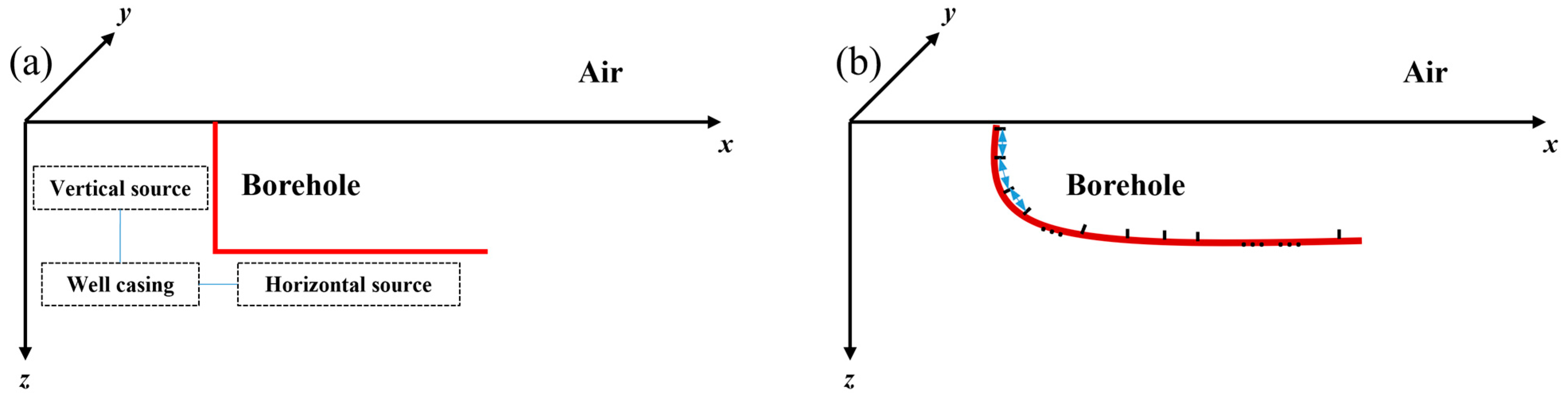
• Based on the developed frequency-domain borehole-to-surface electromagnetic 3D forward algorithm, this paper discusses the optimal method for simulating the transmitter source and conducts correctness verification of the program. A simulation method for constructing complex line sources using the borehole trajectory data of actual wells is proposed. By decomposing highly deviated wells and horizontal wells into vertical and horizontal line sources, the influence of different observation modes with varying transmitter source (B-pole) positions on surface responses is studied, proving that placing the B pole along the borehole trajectory extension direction is the optimal observation mode.
• The surface responses of line sources at a certain depth underground are studied, verifying the effectiveness of the frequency-domain borehole-to-surface electromagnetic observation system, and it is concluded that the optimal surface receiving data is the Ex and Hy components. For fracturing operations, this study verifies the effectiveness of borehole-to-surface electromagnetic method monitoring through borehole-to-surface observation modes and forward numerical simulations. In the simulation of fracturing operations in complex undulating formation models, the fracturing fracture bodies are set, proving the high observation accuracy of surface differential responses of the frequency-domain BSEM method.
• This study verifies the high sensitivity of the frequency-domain BSEM method to monitor changes during the fracturing process through forward simulation cases. By selecting surface electromagnetic field component data at appropriate monitoring frequencies, the development of fractures and fracturing effects can be understood in real time. These research results provide a scientific basis and practical guidance for the setup of borehole-to-surface electromagnetic systems in different scenarios.

In summary, the application of BSEM imaging in dynamic monitoring of actual wells—including water or gas injection, gas storage reservoir operations, and hydraulic fracturing—demonstrates efficiency in subsurface dynamic characterization, highlighting its broad prospects for deep borehole monitoring [55,56,61].

References

1. Mizunaga, H.; Ushijima, K. Three-Dimensional numerical modeling for the mise-a-la-masse method. Geophys. Explor. (Butsurib-Tansa) 1991, 44, 215–226. [Google Scholar]
2. Ushijima, K.; Mizunaga, H.T.; Tanaka, T. Reservoir Monitoring by a 4-D Electrical Technique. Lead. Edge 1999, 18, 1422–1424. [Google Scholar] [CrossRef]
3. Zhang, Y.Y.; Liu, D.J.; Ai, Q.H.; Qin, M.J. 3D modeling and inversion of electrical resistivity tomography using steel cased boreholes as electrodes. J. Appl. Geophys. 2014, 109, 292–300. [Google Scholar] [CrossRef]
4. Tafti, T.A.; Sahimi, M.; Aminzadeh, F.; Sammis, C.G. Use of microseismicity for determining the structure of the fracture network of large-scale porous media. Phys. Rev. E 2013, 87, 032152. [Google Scholar] [CrossRef]
5. Palisch, T.; Al-Tailji, W.; Bartel, L.; Cannan, C.; Zhang, J.; Czapski, M.; Lynch, K. Far-Field Proppant Detection Using Electromagnetic Methods: Latest Field Results. SPE Prod. Oper. 2018, 33, 557–568. [Google Scholar] [CrossRef]
6. Ry, R.V.; Septyana, T.; Widiyantoro, S.; Nugraha, A.; Ardjuna, A. Borehole microseismic imaging of hydraulic fracturing: A pilot study on a coal bed methane reservoir in Indonesia. J. Eng. Technol. Sci. 2019, 51, 251–271. [Google Scholar] [CrossRef]
7. Hu, Y.; Yang, D.; Li, Y.; Wang, Z.; Lu, Y. 3-D Numerical Study on Controlled Source Electromagnetic Monitoring of Hydraulic Fracturing Fluid with the Effect of Steel-Cased Wells. IEEE Trans. Geosci. Remote Sens. 2022, 60, 1–10. [Google Scholar] [CrossRef]
8. Alfano, L. Geoelectric prospecting with underground electrodes. Geophys. Prospect. 1961, 10, 290–303. [Google Scholar] [CrossRef]
9. Snyder, D.D.; Merkel, R.M. Analytic models for the interpretation of electrical surveys using buried current electrodes. Geophysics 1973, 38, 513–529. [Google Scholar] [CrossRef]
10. Merkel, R.H. Resistivity analysis for plane-layer half-space models with buried current sources. Geophys. Prospect. 1971, 19, 626–639. [Google Scholar] [CrossRef]
11. Kaufman, A.A. The electrical field in a borehole with a casing. Geophysics 1990, 55, 29–38. [Google Scholar] [CrossRef]
12. Kaufman, A.A.; Wightman, E.W. A transmission-line model for electrical logging through casing. Geophysics 1993, 58, 1739. [Google Scholar] [CrossRef]
13. Schenkel, C.J.; Morrison, H.F. Electrical resistivity measurement through metal casing. Geophysics 1994, 59, 1072–1082. [Google Scholar] [CrossRef]
14. Wilt, M.; Alumbaugh, D. Oil field reservoir characterization and monitoring using electromagnetic geophysical techniques. J. Pet. Sci. Eng. 2003, 39, 85–97. [Google Scholar] [CrossRef]
15. Tsourlos, P.; Ogilvy, R.; Papazachos, C.; Meldrum, P. Measurement and inversion schemes for single borehole-to-surface electrical resistivity tomography surveys. J. Geophys. Eng. 2011, 8, 487–497. [Google Scholar] [CrossRef]
16. Hoversten, G.M.; Commer, M.; Haber, E.; Schwarzbach, C. Hydrofrac monitoring using ground time-domain electromagnetics. Geophys. Prospect. 2015, 63, 1508–1526. [Google Scholar] [CrossRef]
17. Yang, K.; Torres-Verdín, C.; Yılmaz, A.E. Detection and quantification of three-dimensional hydraulic fractures with horizontal borehole resistivity measurements. IEEE Trans. Geosci. Remote Sens. 2015, 53, 4605–4615. [Google Scholar] [CrossRef]
18. Weiss, C.J.; Aldridge, D.F.; Knox, H.A.; Schramm, K.A.; Bartel, L.C. The direct-current response of electrically conducting fractures excited by a grounded current source. Geophysics 2016, 81, E201–E210. [Google Scholar] [CrossRef]
19. Fang, Y.; Dai, J.; Yu, Z.; Zhou, J.; Liu, Q.H. Through-casing hydraulic fracture evaluation by induction logging I: An efficient EM solver for fracture detection. IEEE Trans. Geosci. Remote Sens. 2017, 55, 1179–1188. [Google Scholar] [CrossRef]
20. Dai, J.; Fang, Y.; Zhou, J.; Liu, Q.H. Analysis of electromagnetic induction for hydraulic fracture diagnostics in open and cased boreholes. IEEE Trans. Geosci. Remote Sens. 2018, 56, 264–271. [Google Scholar] [CrossRef]
21. Kim, J.; Um, E.S.; Moridis, G.J. Integrated simulation of vertical fracture propagation induced by water injection and its borehole electromagnetic responses in shale gas systems. J. Pet. Sci. Eng. 2018, 165, 13–27. [Google Scholar] [CrossRef]
22. Yan, L.J.; Chen, X.X.; Tang, H.; Xie, X.B.; Zhou, L.; Hu, W.B.; Wang, Z.X. Continuous TDEM for monitoring shale hydraulic fracturing. Appl. Geophys. 2018, 15, 26–34. [Google Scholar] [CrossRef]
23. Fang, Y.; Dai, J.; Zhan, Q.; Hu, Y.; Liu, Q.H. A hybrid 3-D electromagnetic method for induction detection of hydraulic fractures through a tilted cased borehole in planar stratified media. IEEE Trans. Geosci. Remote Sens. 2019, 57, 4568–4576. [Google Scholar] [CrossRef]
24. Wilt, M.J.; Um, E.S.; Nichols, E.; Weiss, C.J.; Nieuwenhuis, G.; MacLennan, K. Casing integrity mapping using top-casing electrodes and surface-based electromagnetic fields. Geophysics 2020, 85, E1–E13. [Google Scholar] [CrossRef]
25. Li, Y.; Yang, D. Electrical imaging of hydraulic fracturing fluid using steel-cased wells and a deep-learning method. Geophysics 2021, 86, E315–E332. [Google Scholar] [CrossRef]
26. Wilt, M.; Alumbaugh, D. Electromagnetic Methods for Development and Production: State of the art. Lead. Edge 1998, 17, 487–490. [Google Scholar] [CrossRef]
27. Yee, K. Numerical solution of initial boundary value problems involving maxwell’s equations in isotropic media. IEEE Trans. Antennas Propag. 1966, 14, 302–307. [Google Scholar]
28. Wait, J.R. Some solutions for electromagnetic problems involving spheroidal, spherical, and cylindrical bodies. J. Res. Natl. Bur. Stand. Sect. B Math. Math. Phys. 1960, 64B, 15–32. [Google Scholar] [CrossRef]
29. Weiland, T. A Discretization Method for the Solution of Maxwell’s Equations for Six-Component Fields. Electron. C (AEU) 1977, 31, 116–120. [Google Scholar]
30. Weiss, C.J. Finite-element analysis for model parameters distributed on a hierarchy of geometric simplices. Geophysics 2017, 82, E155–E167. [Google Scholar] [CrossRef]
31. Li, Y.; Spitzer, K. Finite element resistivity modeling for three dimensional structures with arbitrary anisotropy. Phys. Earth Planet. Interiors. 2005, 150, 15–27. [Google Scholar] [CrossRef]
32. Blome, M.; Maurer, H.R.; Schmidt, K. Advances in three-dimensional geoelectric forward solver techniques. Geophys. J. Int. 2009, 176, 740–752. [Google Scholar] [CrossRef]
33. Dey, A.; Morrison, H.F. Resistivity modeling for arbitrarily shaped three-dimensional structures. Geophysics 1979, 44, 753–780. [Google Scholar] [CrossRef]
34. Clemens, M.; Weiland, T. Discrete Electromagnetism with the Finite Integration Technique. J. Electromagn. Waves Appl. 2001, 15, 79–80. [Google Scholar] [CrossRef]
35. Hong, D.; Xiao, J.; Zhang, G.; Yang, S. Characteristics of the sum of cross-components of triaxial induction logging tool in layered anisotropic formation. IEEE Trans. Geosci. Remote Sens. 2014, 52, 3107–3115. [Google Scholar] [CrossRef]
36. Rocroi, J.P.; Koulikov, A.V. The Use of Vertical Line Sources in Electrical Prospecting for Hydrocarbon. Geophys. Prospect. 1985, 33, 138–152. [Google Scholar] [CrossRef]
37. King, R.W.P.; Wu, T.T. The complete electromagnetic field of a three-phase transmission line over the earth and its interaction with the human body. J. Appl. Phys. 1995, 78, 668–683. [Google Scholar] [CrossRef]
38. Wait, J.R. Note on: Fields of a horizontal wire antenna over a layered half-space. J. Electromagn. Wave 1996, 10, 1655–1662. [Google Scholar] [CrossRef]
39. Rucker, C.; Gunther, T.; Spitzer, K. Three-dimensional modeling and inversion of dc resistivity data incorporating topography m I. Modelling. Geophys. J. Int. 2006, 166, 495–505. [Google Scholar] [CrossRef]
40. Pardo, D.; Torres-Verdín, C.; Demkowicz, L.F. Feasibility study for 2D frequency-dependent electromagnetic sensing through casing. Geophysics 2007, 72, F111–F118. [Google Scholar] [CrossRef]
41. Cuevas, N.H.; Pezzoli, M. On the effect of the metal casing in surface-borehole electromagnetic methods. Geophysics 2018, 83, E173–E187. [Google Scholar] [CrossRef]
42. Kohnke, C.; Liu, L.; Streich, R.; Swidinsky, A. A method of moments approach to model the electromagnetic response of multiple steel casings in a layered Earth. Geophysics 2018, 83, WB81–WB96. [Google Scholar] [CrossRef]
43. Stumpf, I. Pulsed vertical-electric-dipole excited voltages on transmission lines over a perfect ground—A closed-form analytical description. IEEE Antennas Wirel. Propag. Lett. 2018, 17, 1656–1658. [Google Scholar] [CrossRef]
44. Yang, D.; Oldenburg, D.W. Electric field data in inductive source electromagnetic surveys. Geophysics 2018, 66, 207–225. [Google Scholar] [CrossRef]
45. Yang, D.; Oldenburg, D.W. Survey decomposition: A scalable framework for 3D controlled-source electromagnetic inversion. Geophysics 2016, 81, E69–E87. [Google Scholar] [CrossRef]
46. Heagy, L.J.; Oldenburg, D.W. Direct current resistivity with steel-cased wells. Geophys. J. Int. 2019, 219, 1–26. [Google Scholar] [CrossRef]
47. Heagy, L.J.; Oldenburg, D.W. Modeling electromagnetics on cylindrical meshes with applications to steel-cased wells. Comput. Geosci. 2019, 125, 115–130. [Google Scholar] [CrossRef]
48. Orujov, G.; Anderson, E.; Streich, R.; Swidinsky, A. On the electromagnetic response of complex pipeline infrastructure. Geophysics 2020, 85, E241–E251. [Google Scholar] [CrossRef]
49. Pardo, D.; Torres-Verdín, C.; Zhang, Z. Sensitivity study of borehole-to-surface and crosswell electromagnetic measurements acquired with energized steel casing to water displacement in hydrocarbon-bearing layers. Geophysics 2008, 73, F261–F268. [Google Scholar] [CrossRef]
50. Pardo, D.; Torres-Verdín, C. Sensitivity analysis for the appraisal of hydrofractures in horizontal wells with borehole resistivity measurements. Geophysics 2013, 78, D209–D222. [Google Scholar] [CrossRef]
51. Barsukov, P.O.; Fainberg, E.B. The field of the vertical electric dipole immersed in the heterogeneous half-space. Izv.-Phys. Solid Earth 2014, 50, 568–575. [Google Scholar] [CrossRef]
52. Sami, G.M.; Al-Najim, F.A. The Transient Electromagnetic Field Created by Electric Line Source on a Plane Conducting Earth. Int. J. Mech. Appl. 2015, 5, 16–22. [Google Scholar]
53. Tietze, K.; Ritter, O.; Veeken, P. Controlled-source electromagnetic monitoring of reservoir oil saturation using a novel borehole-to-surface configuration. Geophysics 2015, 63, 1468–1490. [Google Scholar]
54. Commer, M.; Hoversten, G.M.; Um, E.S. Transient-electromagnetic finite-difference time-domain Earth modeling over steel infrastructure. Geophysics 2015, 80, E147–E162. [Google Scholar] [CrossRef]
55. Tang, W.; Li, Y.; Swidinsky, A.; Liu, J. Three-dimensional controlled-source electromagnetic modelling with a well casing as a grounded source: A hybrid method of moments and finite element scheme. Geophys. Prospect. 2015, 63, 1491–1507. [Google Scholar] [CrossRef]
56. Zhang, W.; Liu, Q.H. Three-dimensional scattering and inverse scattering from objects with simultaneous permittivity and permeability contrasts. IEEE Trans. Geosci. Remote Sens. 2015, 53, 429–439. [Google Scholar] [CrossRef]
57. Sun, Q.; Zhang, R.; Zhan, Q.; Liu, Q.H. Multiscale hydraulic fracture modeling with discontinuous Galerkin frequency-domain method and impedance transition boundary condition. IEEE Trans. Geosci. Remote Sens. 2017, 55, 6566–6573. [Google Scholar] [CrossRef]
58. Fang, Y.; Hu, Y.; Zhan, Q.; Liu, Q.H. Electromagnetic forward and inverse algorithms for 3-D through-casing induction mapping of arbitrary fractures. IEEE Geosci. Remote Sens. Lett. 2018, 15, 996–1000. [Google Scholar] [CrossRef]
59. Um, E.S.; Kim, J.; Wilt, M.J.; Commer, M.; Kim, S.S. Finite-element analysis of top-casing electric source method for imaging hydraulically active fracture zones. Geophysics 2019, 84, E23–E35. [Google Scholar] [CrossRef]
60. Um, E.S.; Kim, J.; Wilt, M. 3D borehole-to-surface and surface electromagnetic modeling and inversion in the presence of steel infrastructure. Geophysics 2020, 85, E139–E152. [Google Scholar] [CrossRef]
61. Bergmann, P.; Ivandic, M.; Norden, B.; Rücker, C.; Kiessling, D.; Lüth, S.; Schmidt-Hattenberger, C.; Juhlin, C. Combination of Seismic Reflection and Constrained Resistivity Inversion with an Application to 4D Imaging of the CO2 Storage Site, Ketzin, Germany. Geophysics 2014, 79, B37–B50. [Google Scholar] [CrossRef]
62. Mulder, W.A. A multigrid solver for 3D electromagnetic diffusion. Geophys. Prospect. 2006, 54, 633–649. [Google Scholar] [CrossRef]
Figure 1. Hydraulic fracturing monitoring by Borehole-to-Surface electromagnetic imaging.
Applsci 15 08312 g001
Figure 2. The borehole-to-surface electromagnetic imaging observation system.
Applsci 15 08312 g002
Figure 3. Configuration of electromagnetic fields on grid cells: (a) the arrangement of the electromagnetic field on the grid cells; (b) the distribution of electric field components and magnetic field components.
Applsci 15 08312 g003
Figure 4. Schematic diagram of well trajectory model decomposition: (a) simplification of well trajectory model decomposition; (b) complex well trajectory model decomposition.
Applsci 15 08312 g004
Figure 5. Half-space model: (a) formation resistivity setting; (b) fracturing anomaly body configuration.
Applsci 15 08312 g005
Figure 6. Schematic diagram of transmitter source (B electrode) positioning: the B electrode is set in (a) the west direction, (b) the east direction, and (c) the north direction.
Applsci 15 08312 g006aApplsci 15 08312 g006b
Figure 7. Comparison of contour maps of surface electric field components: (a) Ex; (b) Ey.
Applsci 15 08312 g007
Figure 8. Comparison of Ex component responses received on the surface before and after simulated fracturing with and without anomalous bodies: (a,b) the real part of Ex before and after the simulated fracturing; (d,e) the imaginary part of Ex before and after the simulated fracturing; (g,h) the total fields of Ex before and after the simulated fracturing; (c,f,i) are the real part, the imaginary part, and the total of the differential anomaly field, respectively.
Applsci 15 08312 g008
Figure 9. Comparison of Hx component responses received on the surface before and after simulated fracturing with and without anomalous bodies: (a,b) the real part of Hx before and after the simulated fracturing; (d,e) the imaginary part of Hx before and after the simulated fracturing; (g,h) the total fields of Hx before and after the simulated fracturing; (c,f,i) are the real part, the imaginary part, and the total of the differential anomaly field, respectively.
Applsci 15 08312 g009
Figure 10. Comparison of Ex component responses in the longitudinal section before and after simulated fracturing with and without anomalous bodies: (a,b) the real part of Ex before and after the simulated fracturing; (d,e) the imaginary part of Ex before and after the simulated fracturing; (g,h) the total fields of Ex before and after the simulated fracturing; (c,f,i) are the real part, the imaginary part, and the total of the differential anomaly field, respectively.
Applsci 15 08312 g010
Figure 11. Comparison of Hx component responses in the longitudinal section before and after simulated fracturing with and without anomalous bodies: (a,b) the real part of Hx before and after the simulated fracturing; (d,e) the imaginary part of Hx before and after the simulated fracturing; (g,h) the total fields of Hx before and after the simulated fracturing; (c,f,i) are the real part, the imaginary part, and the total of the differential anomaly field, respectively.
Applsci 15 08312 g011
Figure 12. Construction of 3D fracturing model for Well X: (a) a 3D geoelectric model; (b) the 27th or 28th section fracturing model.
Applsci 15 08312 g012
Figure 13. Simulation results of Ex surface response for the 27th section fracturing: (ac) frequencies: 1.25 Hz, (df) frequencies: 2.5 Hz.
Applsci 15 08312 g013
Figure 14. Simulation results of Ex surface response for the 28th section fracturing: (ac) frequency: 1.25 Hz, (df) frequency: 2.5 Hz.
Applsci 15 08312 g014
Disclaimer/Publisher’s Note: The statements, opinions and data contained in all publications are solely those of the individual author(s) and contributor(s) and not of MDPI and/or the editor(s). MDPI and/or the editor(s) disclaim responsibility for any injury to people or property resulting from any ideas, methods, instructions or products referred to in the content.