Electrolytic Plasma Hardening of 20GL Steel: Thermal Modeling and Experimental Characterization of Surface Modification

Abstract

This study investigates the thermal response and surface modification of low-carbon manganese-alloyed 20GL steel during electrolytic plasma hardening. The objective was to evaluate the feasibility of surface hardening 20GL steel—traditionally considered difficult to quench—by combining high-rate surface heating with rapid cooling in an electrolyte medium. To achieve this, a transient two-dimensional heat conduction model was developed to simulate temperature evolution in the steel sample under three voltage regimes. The model accounted for dynamic thermal properties and non-linear boundary conditions, focusing on temperature gradients across the thickness. Experimental temperature measurements were obtained using a K-type thermocouple embedded at a depth of 2 mm, with corrections for sensor inertia based on exponential response behavior. A comparison between simulation and experiment was conducted, focusing on peak temperatures, heating and cooling rates, and the effective thermal penetration depth. Microhardness profiling and metallographic examination confirmed surface strengthening and structural refinement, which intensified with increasing voltage. Importantly, the study identified a critical cooling rate threshold of approximately 50 °C/s required to initiate martensitic transformation in 20GL steel. These findings provide a foundation for future optimization of quenching strategies for low-carbon steels by offering insight into the interplay between thermal fluxes, surface kinetics, and process parameters.

1. Introduction

In modern materials science and mechanical engineering, there is a persistent interest in developing effective methods for local hardening of the surfaces of structural steels. The quality and properties of the surface layer are key determinants of wear resistance, corrosion resistance, fatigue resistance, and the overall service life of a product. Electrolytic plasma treatment (EPT) is a promising area in the field of surface engineering, based on the interaction of an electric discharge with the surface of a conductive material immersed in an electrolyte.

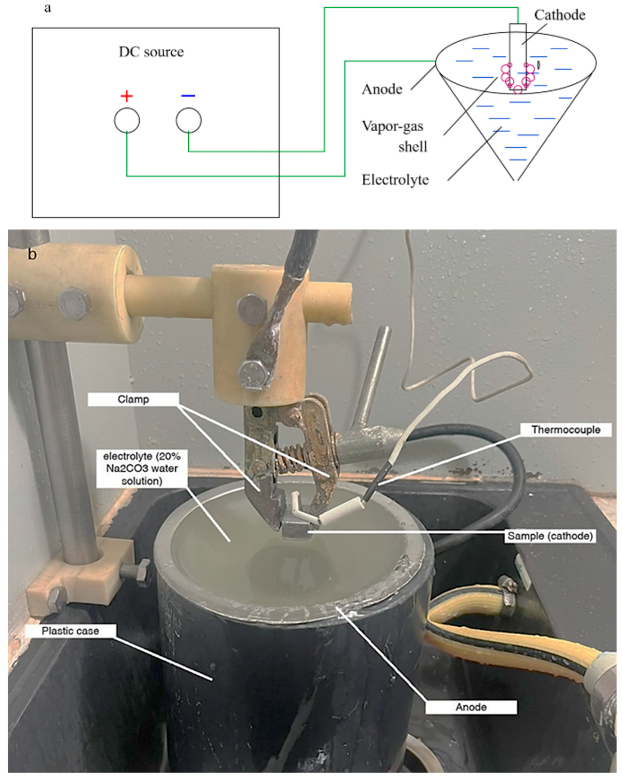
EPT relies on the creation of a plasma discharge between a metallic workpiece, acting as the cathode, and a liquid electrolyte. Upon exceeding a critical voltage (usually 120–400 V), a localized plasma sheath forms around the cathode, achieving temperatures in the range of 5000–8000 K [1]. This discharge induces a significant thermal impact on the material’s surface, causing rapid heating, followed by immediate cooling in the electrolyte, leading to surface hardening and the formation of a hardened microstructure.

Of particular interest is the application of EPT to structural cast steel 20GL, prized for its high processability, strength, and availability. While 20GL steel is normally weakly susceptible to thermal hardening because of its low carbon content (~0.2%) and the prevalence of a ferrite–pearlite structure, the rapid heating and cooling rates in the EPT process can make it possible to achieve austenitization of the surface layer. This leads to the formation of a hardened structure after quenching, opening avenues for enhancing the wear and corrosion resistance of cast parts without significantly complicating their manufacturing technology.

In the work [2], it was demonstrated that increasing the heating rate significantly expands the temperature range in which the phase transformation occurs, specifically the transition from ferrite to austenite. The author also indicated that even with the complete disappearance of ferrite, regions with a high carbon concentration may persist around former carbide particles. These carbon-rich areas can undergo hardening during rapid cooling, as demonstrated on 20GL steel.

Electrolytic plasma treatment, in all its variations, employs high-speed heating methodologies. Some works [3,4] indicate that cathode heating can yield heating rates ranging from 10 to 200 °C/s under constant voltage conditions. Furthermore, the cooling rate of the component following cathodic heating can be controlled via adjustments to the applied voltage, spanning from 12 to 80 °C/s within the zone of minimal austenite stability and from 20 to 140 °C/s in the martensitic transformation range [5].

Continuing the development of research in the field of electrolytic plasma treatment, it is important to note that the thermal processes occurring in the near-surface layer of the metal play a key role in shaping the structure and properties of the processed material [6]. The temperature mode of heating determines the depth and nature of phase transformations, while the cooling rate dictates the possibility of forming hardened structures, such as martensite. Therefore, a quantitative assessment of temperature, heat flow, as well as heating and cooling rates, holds significant practical importance, enabling the prediction of thermal hardening effectiveness across various processing modes.

Several studies [7,8,9,10] have explored the thermal and electrophysical phenomena that occur during anodic electrolytic plasma heating, including the modeling of temperature fields, heat flux density distribution, and electric potential within the electrolyte bath. These investigations have determined that the intensity of thermal exposure and the nature of plasma formation are influenced by factors such as the geometry of the treated component, the type of electrolyte used, the electrode material, and the applied voltage regime. However, the cathodic variant of electrolytic plasma treatment, specifically concerning the thermal state of the surface and its relationship to surface hardening, remains insufficiently studied [11,12]. One attempt to analyze the temperature field during cathodic EPT was conducted in [13], where an analytical solution was put forth based on the assumption of constant thermal conductivity. Nevertheless, when considering the temperature dependence of thermal conductivity, the analytical formulation becomes considerably more complex, rendering the approach suggested previously inapplicable.

Cathodic heating in aqueous electrolytes is distinguished by a high density of thermal action concentrated on a limited area, rendering it particularly advantageous for the localized thermal modification of steels, including those with low-carbon content. Despite the presence of individual experimental studies, a systematic analysis of thermal processes during cathodic electrolytic plasma treatment of 20GL steels is lacking. Consequently, quantitative models that correlate voltage modes and pulse duration with surface temperature, heat flow, and subsequent changes in hardness and microstructure have not been developed.

The aim of this work is to evaluate, both numerically and experimentally, the thermal processes occurring in the near-surface zone of 20GL steel during cathodic electrolytic plasma treatment. This assessment includes a study of the relationship between voltage modes, heating and cooling rates, hardness, and microstructural changes. Three voltage levels—150 V, 200 V, and 250 V—were selected as the modes to be studied, with a constant treatment duration applied. This will allow for an estimation of the heating and cooling rates during cathodic EPT using experimental data on the heat flux, and will also enable a comparison of the numerically calculated surface temperature with the characteristics of the hardened layer.

2. Materials and Methods

2.1. Experimental Approach

The experiments were conducted at the Engineering Center of the Shakarim University in Semey. An experimental setup for electrolytic plasma treatment was constructed, and its schematic representation is provided in Figure 1a. This setup comprised a 50 kW DC source, an electrolyte bath, an electric pump, and a cone-shaped stainless steel anode through which the electrolyte was supplied. A 20% aqueous solution of sodium carbonate (Na₂CO₃) served as the electrolyte. The samples, made of 20GL steel, were prepared as parallelepipeds and manually polished using sandpaper with progressively finer grit sizes, ranging from P100 to P2500. The samples had the following geometric dimensions: a length of 25 mm, a width of 20 mm, and a height of 15 mm. The electrolyte flow rate was 10 L/min. The electrolyte flow rate was measured using an electronic meter, the Piusi K24 Meter (Piusi, Suzzara, Italy).

To evaluate the overall structure, a metallographic microscope HL-102AW (Shanghai Hualong Test Instruments Corporation, Shanghai, China) was utilized. For metallographic microanalysis, sections of steel samples were polished using chromium dioxide paste and subsequently etched with a 4% alcohol solution of nitric acid. The microhardness of the steel samples was then measured using an HV-1 DT device (Shanghai Hualong Test Instruments Corporation, Shanghai, China), with an indenter load of p = 1 N and a holding time of 10 s (in accordance with the requirements of GOST 9450-76).

The electrolyte temperature following each hardening cycle was measured using an LT-300 (Thermex, Tosno, Russia) laboratory electronic thermometer, which has a measurement range of −50 °C to +300 °C and a division value of 0.01 °C. Measurements were taken by immersing the thermometer probe into the electrolyte solution after each hardening stage.

During electrolytic plasma hardening (EPH), the current and voltage values in the electrolytic cell were recorded using an analog signal measurement circuit. Voltage was read via a PC817 optocoupler (Sharp Microelectronics, Sakai, Osaka, Japan), and current strength was read using an SCT-013-000 current transformer (Shenzhen Zhuang Yi Electronics Technology, Shenzhen, China). Both signals were fed to an ATmega328P microcontroller (Microchip Technology Inc., Chandler, AZ, USA) for primary processing. The sample temperature was monitored using a MEGEON26003 K-type thermocouple (MEGEON, Omsk, Russia) with a measurement range of (−50…+1200) °C and a MAX6675 digital module (Shenzhen Qinyuansheng Electronics, Shenzhen, China). The data from the thermocouple and module were also transmitted in digital form to the microcontroller for primary processing. The thermocouple was installed in the sample at a distance of 2 mm from the surface through a hole in the back of the sample (Figure 1b). All obtained parameters—current, voltage, and temperature—were transmitted to a personal computer, where they were saved for subsequent analysis and processing.

The electrical schematic diagram of the measuring system used to register the parameters of the EPH process is illustrated in Figure 2. This diagram was divided into three functional sections. Section A measures the voltage in the electrolyte circuit, using a PC817 optocoupler for galvanic isolation and safe transmission of the analog signal to the ATmega328P microcontroller. Section B measures current with an SCT-013-000 current sensor, which converts the current value into an analog signal that is then fed to the ADC input of the microcontroller. Lastly, Section C regulates temperature using the MEGEON26003 thermocouple connected to the MAX6675 digital module, which converts the thermocouple signal into digital format before transmitting it to the microcontroller.

Despite certain limitations associated with thermal lag and potential contact resistance, the selected temperature measurement method was deemed the most reliable under the conditions of electrolytic plasma treatment. The use of non-contact techniques, such as infrared pyrometry, is challenging in the context of EPT due to the nonequilibrium and unstable nature of the radiation emitted by the cathodic plasma, which can cause significant interference with the signal and lead to inaccurate surface temperature readings.

Furthermore, pyrometers generally exhibit significantly higher measurement uncertainty—typically within several degrees—whereas contact thermocouples provide precision down to tenths or even hundredths of a degree, especially when properly calibrated and digitally filtered. Infrared methods also lag behind thermocouples in terms of response time, which is critical for capturing rapid thermal dynamics characteristic of EPT processes.

2.2. Energy Balance

In order to study the effect of electrolytic plasma hardening for 10 s on the temperature distribution in 20GL steel samples in three modes of 150 V, 200 V and 250 V, the values of the amount of heat released during the current flow during EPT were calculated for each of the three modes. The amount of heat, in turn, was calculated based on the dynamics of electric power during EPT by integrating the function P(t) over time. Since the nature of the function P(t) was complex with many local minima and maxima, the integration was carried out using the trapezium formula

$$Q_e\approx {\sum }_{i=0}^{N-1}{P}_i·{∆t}_i\approx {\sum }_{i=0}^{N-1}{\displaystyle \frac{P_i+P_{i+1}}{2}}·{∆t}_i,$$

(1)

where Q_e—amount of heat released during the EPH process; P_i and P_i+1—adjacent values of electric power on the P(t) graph; and ∆t_i—time difference equal to ∆t_i = t_i+1 − t_i and determined separately for each value P_i and P_i+1.

The graphs of the function P(t) were derived by multiplying the corresponding values of the functions I(t) and U(t) using the formula

$$P\left(t\right)=U\left(t\right)·I\left(t\right).$$

(2)

To estimate the heat flux density during electrolytic plasma hardening of 20GL steel, it is necessary to consider the law of conservation of energy. Research [14,15,16] has established that the conversion of electrical energy into heat occurs in the plasma layer on the processed surface of the cathode sample. Based on these assumptions, the energy distribution during EPH of the cathode sample is presented as follows:

$$Q_k= Q_e-Q_v-Q_r-Q_h,$$

(3)

where Q_k—energy spent on heating the plasma layer and the cathode; Q_e—amount of heat calculated using Formula (1); Q_v—energy spent on evaporating the electrolyte; Q_r—radiation energy of the plasma layer; Q_h—energy spent on heating the electrolyte.

It is now necessary to evaluate the terms included in Equation (3). The values for Q_e are obtained from Formula (1). Given that the thickness of the vapor–plasma shell is small compared to its perimeter, the radiation of the plasma layer can be neglected [17], thus Q_r = 0. The term Q_h can be calculated using the formula

$$Q_h=c·m·∆T,$$

(4)

where c—specific heat capacity of the electrolyte solution; m—mass of the entire solution in the reservoir; ∆T—temperature increase during a single quenching of the sample over a time of t = 10 s.

To estimate the heat used for electrolyte evaporation in the cathode area, it is necessary to determine the nature and volume of the vapor–gas envelope formed during electrolytic plasma treatment. According to a number of experimental studies, the vapor–gas envelope at cathodic polarity has a pulsating nature [18,19,20]. Initially, intensive electrolyte evaporation occurs near the cathode, forming a vapor–gas shell. Upon reaching a certain threshold, the shell breaks down and a discharge occurs, destroying the shell. The cycle then repeats, accumulating a new shell. This pulsation was confirmed by oscillographic recordings of current strength and visual observations of the process. On the I graph, each cycle corresponds to the duration between two successive local minima and maxima. This discharge dynamic supports the idea that numerous local phase transitions of liquid into steam occur during the EPT process (for example, lasting 10 s), resulting in shell formation.

Therefore, the heat Q_v should be estimated by considering multiple cycles rather than a single shell volume. The average discharge frequency extracted from the analysis of the I(t) graph can be used to estimate the number of cycles. Consequently, during the processing time, numerous complete cycles of shell accumulation and destruction can be observed, each accompanied by partial evaporation of the electrolyte volume around the cathode. Thus, when calculating the heat Q_v, the number of cycles must be considered by multiplying the heat for one cycle by the total number of cycles N. To estimate the heat spent on forming the vapor–gas shell in one cycle, the geometry and volume of the evaporating near-cathode zone must be specified. According to [21,22], the thickness of the vapor–gas shell ranges from 50 to 200 μm, depending on the voltage and electrolyte modes. In this work, an average shell thickness parameter of δ = 100 μm was adopted for the assessment.

Considering this thickness for calculations, the cathode evaporation region can be approximated as a volume. This volume was formed by extending the shell from all external boundaries of the sample by a thickness δ and deepening along the normal by the same value. Therefore, if the dimensions of the sample are a × b × h, the volume of the shell can be estimated as

$$V_{vge}=(a+2\delta )·(b+2\delta )·\delta ,$$

(5)

where δ—thickness of the vapor–gas shell; a and b—length and width of the sample, respectively.

This approximation provides insight into the zone where the phase transition of liquid into steam occurs due to local heating. Consequently, the heat of evaporation in one cycle can be determined using the following formula:

$$Q_v^{\left(1\right)}=\rho ·V_{vge}·L,$$

(6)

where ρ—density of the electrolyte; L—specific heat of vaporization of the electrolyte solution. Therefore, the total amount of heat for electrolyte evaporation in the cathode region during hardening can be estimated as

$${Q_v=N·Q}_v^{\left(1\right)}=N·\rho ·V_{vge}·L.$$

(7)

2.3. Estimation of Heat Fluxes

After evaluating all the terms on the right-hand side of (3), the value of Q_k is determined. To assess the degree of thermal impact on the material and construct temperature profiles, it is advisable to calculate the heat flux density. The average heating power of the cathode was then determined as

$$P_k={\displaystyle \frac{Q_k}{t}},$$

(8)

where P_k—average heating power of the cathode over time; t—duration of hardening (10 s). The heat flux density, which corresponds to the average heating power, is then calculated as follows:

$$q={\displaystyle \frac{P_k}{S}},$$

(9)

where S—area of the contact surface of the sample with the electrolyte.

At the same location where the heat flux q is applied, intense heat exchange with the surrounding electrolyte also takes place. The electrolyte washes the lower surface of the sample, removing heat through convection. Consequently, the temperature distribution within the material was formed by the interaction of the heating source and the cooling effect of convective heat exchange.

To correctly take this effect into account in numerical modeling, it is necessary to determine the heat transfer coefficient α. This coefficient relates the heat flow to the temperature difference between the sample and the electrolyte, as described by Newton–Richmann’s law:

$$q_c=\alpha ·(T_{surf}-T_{el}),$$

(10)

where q_c—density of heat flow going into the electrolyte; T_surf—surface temperature of the sample; T_el—electrolyte temperature.

To estimate the heat transfer coefficient, the method of analyzing dimensionless similarity numbers is employed, using Reynolds, Prandtl, and Nusselt numbers. In the scenario where the electrolyte flows out through the upper base of the anode cone and washes the surface of the part from below, followed by radial spreading, the characteristic size used for calculating the similarity numbers will be the average hydraulic size Z (since the surface is a rectangle measuring 20 mm by 25 mm). This size is calculated using the formula

$$Z={\displaystyle \frac{2·a·b}{(a+b)}}.$$

(11)

Since the electrolyte flows out of the upper base of the cone anode with a diameter D, with a flow rate of G = 10 L/min, the flow rate of the electrolyte at the surface of the sample is determined as

$$v={\displaystyle \frac{4·G·{10}^{-3}}{60·\pi ·D^2}} (\mathrm{m}/\mathrm{s}).$$

(12)

Then the Reynolds number is defined as

$$Re={\displaystyle \frac{v·Z}{\nu }},$$

(13)

where υ—flow rate of the electrolyte at the surface of the sample; Z—characteristic size of the streamlined body; ν—kinematic viscosity of the electrolyte solution. The Prandtl number for an electrolyte solution is calculated using the formula

$$Pr={\displaystyle \frac{c·\mu }{\lambda }},$$

(14)

where c—specific heat capacity of the electrolyte solution; μ—dynamic viscosity of the electrolyte solution; λ—thermal conductivity of the electrolyte solution.

The flow characteristics observed in the experiment and subsequent calculations definitively indicate laminar flow within the system under investigation. Based on this, according to the literature [23], the formula for calculating the Nusselt number is as follows:

$$Nu=0.664·{Re}^{0.5}·{Pr}^{1/3}.$$

(15)

This formula is valid for flow around a plate when the Reynolds number is less than 500,000. Following this, the heat transfer coefficient α is determined using the formula

$$\alpha ={\displaystyle \frac{Nu·\lambda }{Z}}.$$

(16)

The required calculation parameters (L, c, λ, ρ, μ, ν) for the sodium carbonate solution were taken from [24].

2.4. Formulation of the Boundary Value Problem

Once the heat flux density q and the heat transfer coefficient α have been determined, and the boundary conditions on the electrolyte side with temperature T_el have been established, we can proceed to the mathematical formulation of the thermal conductivity problem to describe the heating of a metal sample during electrolytic plasma treatment.

A two-dimensional formulation of the non-stationary thermal conductivity problem is considered, accounting for the temperature dependence of thermophysical properties:

$${\rho }_s\left(T\right)·c_s\left(T\right)·{\displaystyle \frac{\partial T}{\partial t}}={\lambda }_s(T)·({\displaystyle \frac{{\partial }^{2}T}{\partial x^2}}+{\displaystyle \frac{{\partial }^{2}T}{\partial y^2}}),$$

(17)

where T = T(x,y,t) is the temperature at point (x,y) at time t, ρ_s is the density of steel, c_s is the specific heat capacity of steel, and λ_s is the thermal conductivity of steel (all properties of steel are functions of temperature).

It is now necessary to define the boundary conditions. For the lower boundary (y = 0),

$$-{\lambda }_s\left(T\right){\left.{\displaystyle \frac{\partial T}{\partial y}}\right|}_{y=0}=q-\alpha ·(T_{surf}-T_{el}),$$

(18)

where the right-hand side takes into account both the external heat flow from the source q and the convective heat transfer into the electrolyte.

The influence of the holder was considered on the lateral surfaces of the sample. The boundary condition for contact with the holder was applied exclusively from the mid-height of the lateral surfaces up to the upper boundary, specifically for x = 0, x = a, and h/2 ≤ y ≤ h. For the upper boundary, as well as in the regions 0 ≤ y ≤ h/2, a condition of zero heat flux was assumed (Figure 3a). Consequently, the boundary conditions are formulated as follows:

$${\left.{\displaystyle \frac{\partial T}{\partial y}}\right|}_{y=h}=0; {\left.{\displaystyle \frac{\partial T}{\partial x}}\right|}_{\begin{array}{c}x=0,\\ yϵ[0,{\displaystyle \frac{h}{2}}]\end{array}}={\left.{\displaystyle \frac{\partial T}{\partial x}}\right|}_{\begin{array}{c}x=a,\\ yϵ[0,{\displaystyle \frac{h}{2}}]\end{array}}=0; {\left.{\displaystyle \frac{\partial T}{\partial x}}\right|}_{\begin{array}{c}x=0,\\ yϵ[{\displaystyle \frac{h}{2}},h]\end{array}}={\left.{\displaystyle \frac{\partial T}{\partial x}}\right|}_{\begin{array}{c}x=a,\\ yϵ[{\displaystyle \frac{h}{2}},h]\end{array}}={\alpha }_{cl}·(T-T_{\infty }),$$

(19)

where ${\alpha }_{cl}$—contact conductivity of the “sample-holder”; T—current temperature on the side surfaces; T_∞—temperature of the holder surrounding the part. As a first approximation, we assume that the holder is a massive body and its temperature does not change much relative to room temperature, so we consider T_∞ = 20 °C.

At the initial time, the sample temperature is assumed to be equal to the ambient temperature:

$$T\left(x,y,0\right)=T_0.$$

(20)

Given that the thermal properties of steel are temperature-dependent, the problem becomes non-linear. Due to the complexity involved, finding an analytical solution to the posed boundary value problem (17)–(20) is challenging; therefore, for our objectives, we will focus on obtaining a numerical solution.

2.5. Numerical Approach

The numerical calculation of the problem was performed in the Elcut 6.6 program [25]. This program is designed to simulate various physical fields using the finite element method (FEM) [26]. Within the Elcut 6.6 software environment, the problem was configured as an “Unsteady Heat Transfer” scenario, utilizing a two-dimensional model and specifying length units in millimeters. The model’s mesh consisted of 254 nodes (Figure 3b). Boundary conditions were defined in the “Edge Labels” section, applying specific conditions to the sides and top of the rectangular geometry. Additionally, a defined heat flux was applied to the lower boundary of the rectangle, representing both the applied heating flux q and the heat exchange with the electrolyte solution, denoted as q_c.

The Elcut software supports automatic mesh generation based on user-defined discretization steps. The user can define the discretization step globally for the entire domain or locally for specific subregions. The discretization step determines the approximate distance between neighboring nodes in the finite element mesh within a given geometric region. By adjusting this parameter, a balance can be achieved between computational accuracy and the total runtime of the simulation.

To assess the influence of mesh resolution on the accuracy of the thermal simulation, a mesh refinement analysis was performed for the 200 V case using three discretization levels: (1) for 254 nodes: the discretization step was 1.31 mm; (2) for 6000 nodes: the discretization step was 0.26 mm; (3) for 40,000 nodes: the discretization step was 0.1 mm. Figure 3c,d illustrate the discretization of the computational model into approximately 6000 and 40,000 mesh nodes, respectively.

In the “Block Labels” section, the temperature-dependent specific heat capacity and thermal conductivity of 20GL steel were specified using data for the thermophysical parameters of low-carbon manganese steel [27]. Time integration was selected based on the processing time condition, set to 10 s with an integration step of 0.01 s. The calculation, performed on a computer with a dual-core Intel Core i3 processor, took approximately 5–7 s for the 254-node model. The program calculated the temperature at each node and constructed a two-dimensional temperature field, ensuring sufficient modeling accuracy for analyzing the temperature field distribution in the sample after hardening.

3. Results and Discussion

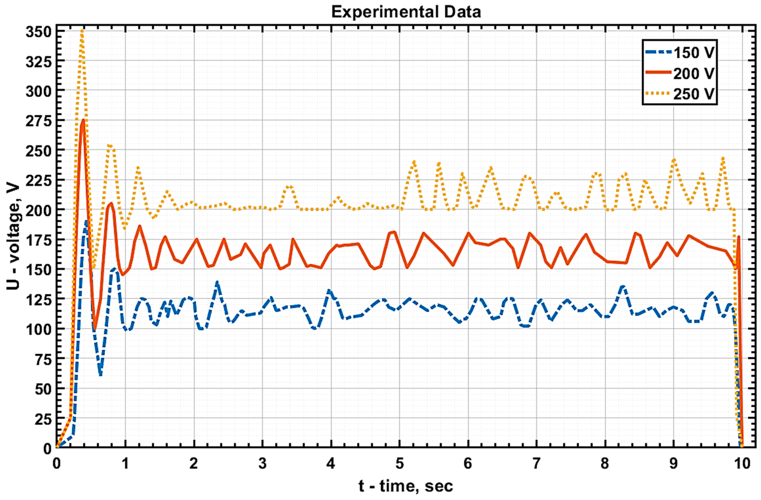
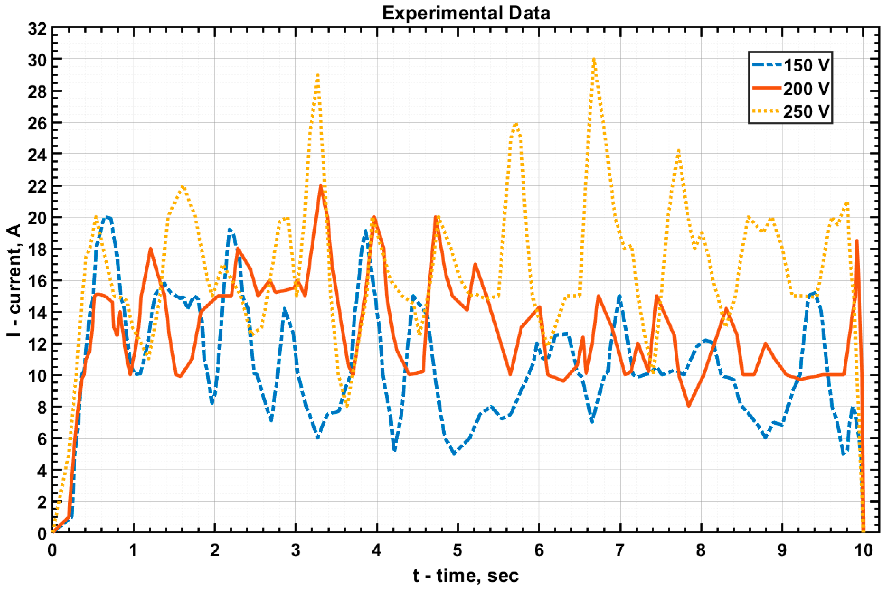
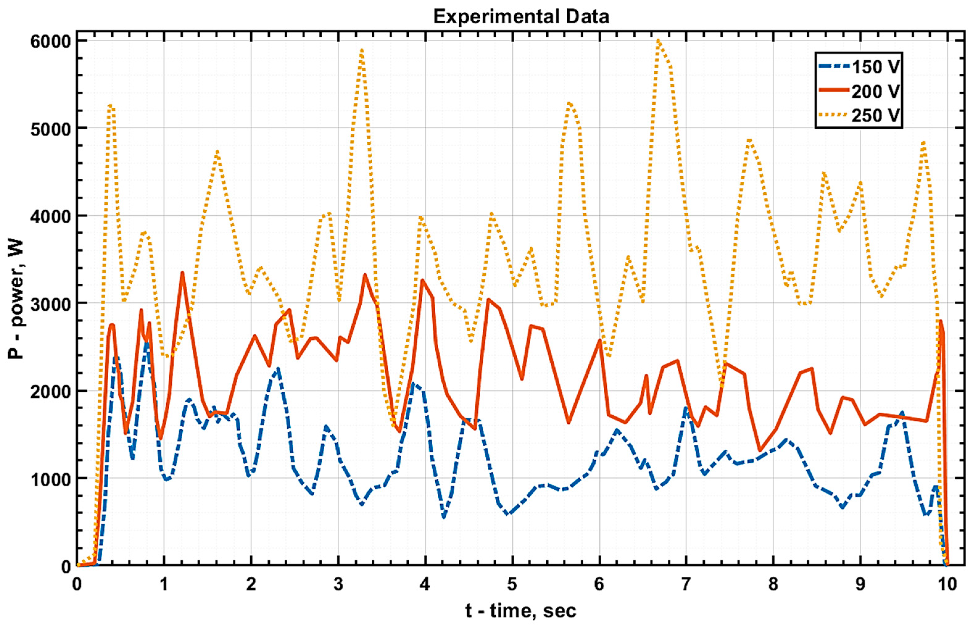
The values of current and voltage at the electrolytic cell were measured, and graphs of U(t), I(t), and P(t) were subsequently plotted based on these measurements (Figure 4, Figure 5 and Figure 6, respectively).

Next, the amount of heat released as a result of the current flow was calculated using Formula (1). The calculation results are presented in

Table 1. Summary energy characteristics of EPH for three modes.

Parameter/Mode	150 V	200 V	250 V
Electrical energy input, Qe, J	12,038 ± 722.2	20,905 ± 1254.3	34,549.5 ± 2072.9
Electrolyte heating, Qh, J	1086.3 ± 152.1	2716.2 ± 380.2	6518.8 ± 912.6
Vaporization heat, Qv, J	2351.1 ± 21.2	2766 ± 24.9	2351.1 ± 21.2
Workpiece heating, Qk, J	8675.6 ± 738.3	15,507.8 ± 1310.9	25,775.6 ± 2265
Heat flux density, q, W/m2	$(17\pm 1.6)·{10}^5$	$(31\pm 2.9)·{10}^5$	$(51\pm 4.9)·{10}^5$
Heat transfer coefficient to electrolyte, α, W/(m2∙K)	339 ± 1.8

.

The electrolyte’s temperature was measured using an LT-300 thermometer (Termex, Tomsk, Russia) to evaluate its heating after processing. Initially, the electrolyte temperature was 20 °C. Following a 10 s hardening process at U = 150 V, the electrolyte temperature reached 20.02 °C. With voltages of 200 V and 250 V, the electrolyte temperature increased to 20.05 °C and 20.12 °C, respectively, after the same duration. The mass of the entire electrolyte solution in the tank was about 15 kg. The obtained values made it possible to calculate the amount of heat Q_h that went into heating the electrolyte using Formula (4) for each of the three hardening modes. The calculation results are shown in Table 1.

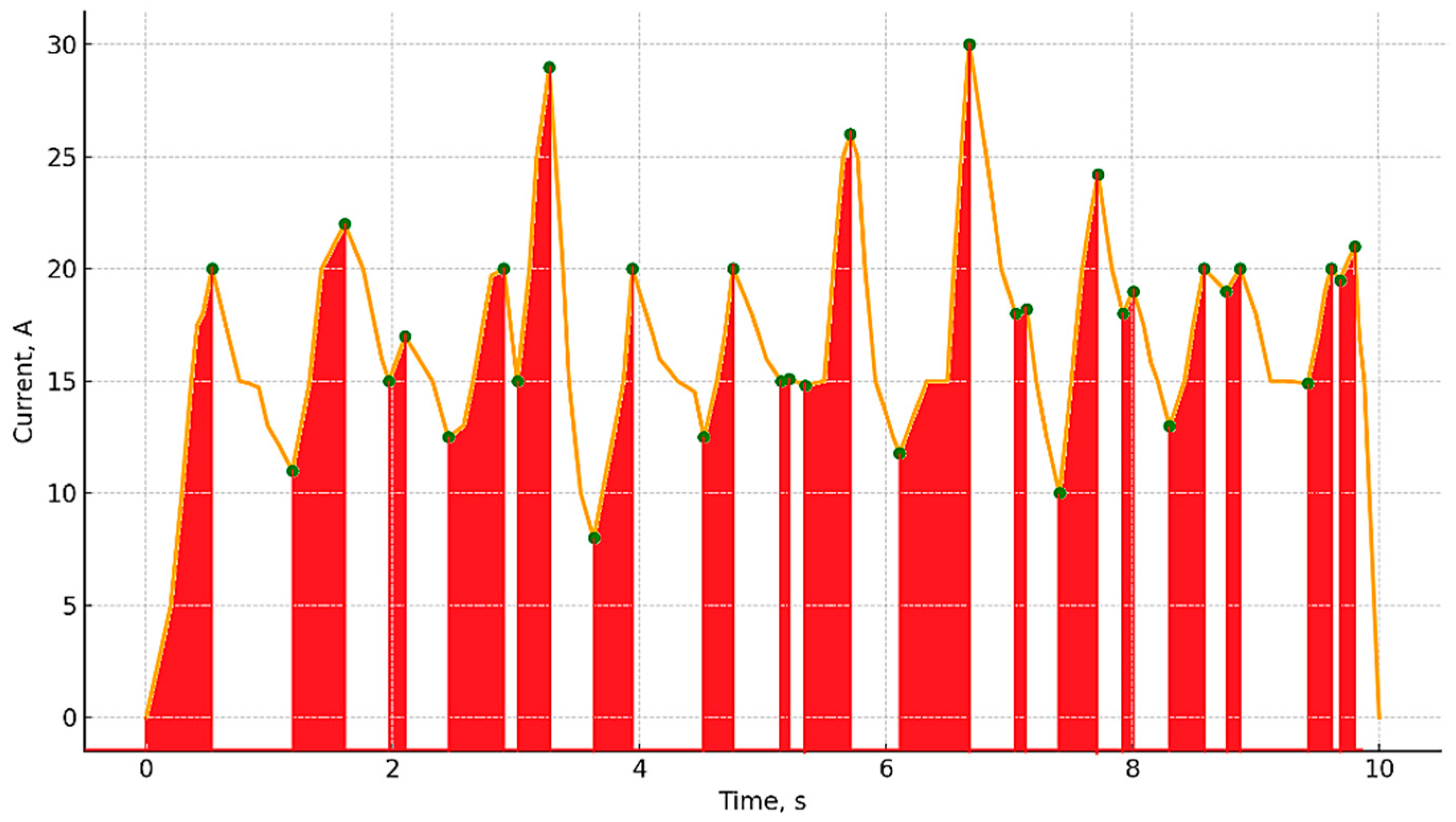
When analyzing the dynamics of the current I(t) in the system, it was found that each single discharge corresponds to a local peak on the experimental curve (Figure 7). Therefore, the average number of pulses in the process can be approximately estimated by the number of pronounced local current maxima within the time interval of processing. Between two adjacent peaks, there are characteristic sections that reflect the vapor–gas shell accumulation stage. This stage is visualized as an interval from a local minimum to the subsequent maximum and can be interpreted as a gradual increase in resistance due to the formation and growth of the shell (red area on the graph). The discharge itself occurs when this shell is broken through and manifests itself as a local current maximum. This is followed by the recovery phase—an area on the graph from a local maximum to a subsequent minimum, reflecting the redistribution of the electric field, stabilization of the system and repeated growth of the shell. Accordingly, for each processing mode, it is possible to estimate the number N of such shell recoveries, which is subsequently used to estimate the amount of heat Q_v that went to electrolyte evaporation. The calculation results are reflected in Table 1.

In Table 1, the calculated values of vaporization heat Q_v for both the 150 V and 250 V regimes appear identical. This was due to the use of the same number of vapor–gas envelope pulsations (N = 17), as observed from current oscillograms, along with identical assumptions for vaporization volume, electrolyte density, and latent heat of vaporization, which were considered approximately constant between the two regimes. Although the input power was different, the frequency and number of pulsation cycles remained similar during the 10 s treatment interval, resulting in comparable cumulative energy expenditure for vapor generation in both cases.

As a first approximation, the holder was considered more massive than the part, and it was assumed that heat dissipation to the holder was more significant than to the surrounding air. It was also assumed that the pressure in the contact zone was moderate, with small oxides and roughness. Under these conditions, the contact conductivity typically ranges from 500 to 2000 W/m·K in the literature [28]. To provide a more physically grounded estimation, we employed the solid-spot contact model proposed by C.V. Madhusudana [29]. This model considers “rough–rough” metal contact, where both surfaces undergo plastic deformation.

In our case, the surface roughness was estimated as Ra ≈ 1 μm for the 20GL steel sample (sides roughly grounded but not polished), and Ra ≈ 3–5 μm for the stainless steel holder (as-manufactured). The contact pressure was estimated to lie between 0.4 and 1.2 MPa, based on the tightening torque (1–1.5 N·m) applied during assembly, assuming a thread friction coefficient of μ ≈ 0.2 and a contact area of 125 mm². According to Madhusudana’s empirical formulation for plastically deformable rough surfaces, the thermal contact conductance can be approximated by

$${\alpha }_{cl}=1150·P^{0.94},$$

(21)

where P—contact pressure, MPa. Substituting the estimated pressure values yields ${\alpha }_{cl}\approx 500-2000 \mathrm{W}/{\mathrm{m}}^2·\mathrm{K}$, which is consistent with the empirical range found in prior experimental and theoretical studies for similar materials and conditions. To validate the robustness of the model, a sensitivity analysis for the U = 200 V regime was performed by varying ${\alpha }_{cl}$ within this range (

Table 2. Effect of contact conductivity ${\alpha }_{cl}$ on the surface and internal temperatures of the sample (U = 200 V).

Contact Conductivity ${\mathit{\alpha }}_{\mathit{c}\mathit{l}}$$,\mathbf{W}/{\mathbf{m}}^2·\mathbf{K}$	T Surface, °C	T Middle, °C	T Back, °C
500	875.45	438.29	335.81
1000	871.28	432.74	329.03
1500	867.15	428.56	322.84
2000	862.63	423.16	316.73

). The results indicated that surface temperatures changed to 12.8 °C, and internal temperatures also remained moderately affected. These findings suggest that the simulation is only weakly sensitive to this parameter, and the selected range is both physically justified and numerically stable. In further numerical calculations, the value of contact conductivity was taken as ${\alpha }_{cl}=500 \mathrm{W}/{\mathrm{m}}^2·\mathrm{K}$.

To enhance the accuracy of the thermal model in the high-temperature regime (U = 250 V), radiative heat losses from the exposed surfaces of the sample were incorporated into the boundary conditions. The radiation condition was written as follows

$$q_r=\epsilon ·{\sigma }_0·(T^4-T_{amb}^4),$$

(22)

where ε—emissivity coefficient; ${\sigma }_0$—Stefan–Boltzmann constant; T—current surface temperature; $T_{amb}$—the temperature of the environment where the radiation goes.

This modification addresses the increasing significance of radiative dissipation above 1000 °C, where the discrepancy between simulated and experimental temperatures becomes more pronounced if radiation is neglected.

Radiation boundary conditions were applied to both the heated surface in contact with the electrolyte and the lateral surfaces exposed to air. The emissivity values were selected based on the surface finish: ε ≈ 0.4–0.5 for the polished working surface and ε ≈ 0.7–0.8 for rougher lateral sides. These values were taken from [30]. The ambient temperature was set to 293 K (20 °C), consistent with the temperature of the circulating electrolyte.

Numerical results demonstrated that accounting for radiation led to a measurable reduction in the calculated surface temperature at U = 250 V, from 1518.5 °C to 1490.6 °C—a difference of approximately 28 °C (1.84%). In contrast, the effect was negligible for lower voltages: 5.9 °C (0.67%) for 200 V, and 1.2 °C (0.25%) for 150 V.

Given these results, radiative losses were included in the model only for the 250 V mode, where their impact on accuracy is most significant. For lower-voltage modes, radiation was omitted to avoid unnecessary model complexity, as its influence on the results was within the numerical error margin.

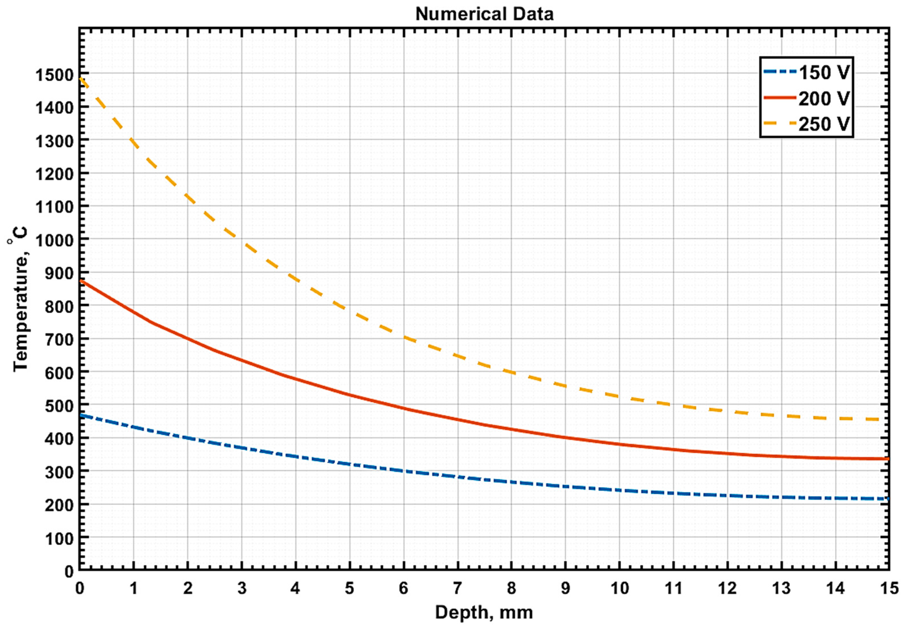
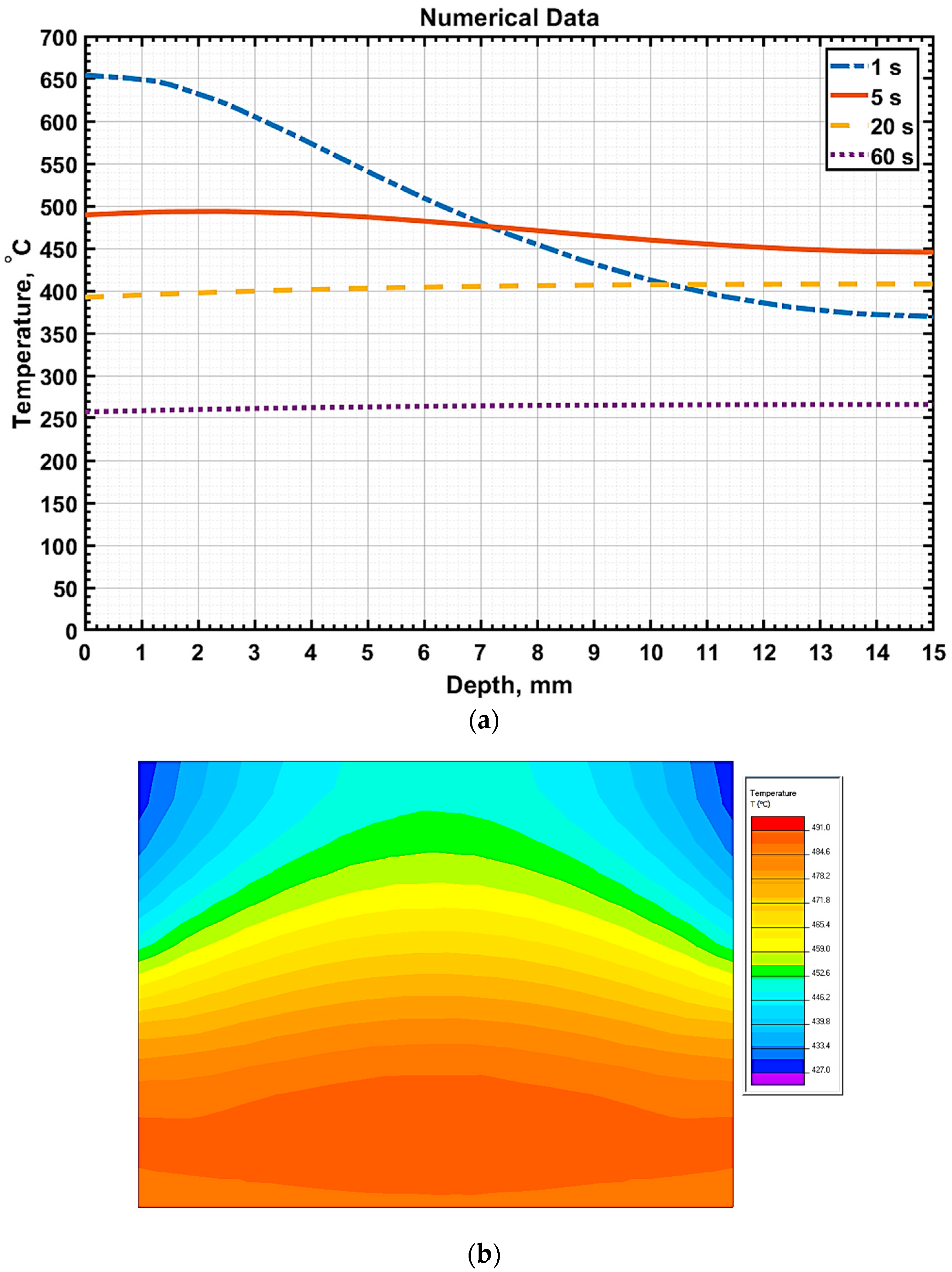
After calculating and summarizing all energy terms in Table 1, these values were used to define the third kind of boundary conditions in the Elcut 6.6 program. Figure 8 illustrates the temperature distribution graphs along the sample depth at t = 10 s for three processing modes of 20GL steel, measured precisely along the line x = a/2, which is at the sample’s midpoint.

Following the heating phase, the cooling of the part after voltage removal was simulated using the Elcut 6.6 program, with q = 0 while maintaining the established boundary conditions. Figure 9a depicts the temperature distribution pattern relative to the sample’s depth (on the line x = a/2) during cooling at different time intervals, as well as the temperature distribution pattern across the sample’s cross-section 5 s after the voltage was disconnected (Figure 9b).

To ensure a valid comparison, the numerical calculation results were analyzed at a depth of 2 mm, consistent with the experimental temperature measurements obtained using a thermocouple. However, the interpretation of experimental data must consider the inherent measurement inertia; the MEGEON26003 thermocouple’s response time is approximately 4 s, according to its technical specifications. Consequently, the thermocouple readings may lag behind the actual temperature of the sample, particularly under the rapid heating conditions characteristic of electrolytic plasma hardening.

To estimate this delay, a classical model, described by a linear differential equation of the first order, was used to represent the response of the inertial measuring device. The solution to such an equation is an exponential approximation:

$$T_{tc}\left(t\right)=T_{real}(t)·(1-e^{-{\displaystyle \frac{t}{\tau }}}),$$

(23)

where T_tc represents the thermocouple reading, T_real represents the true temperature within the sample, t is the current time, and τ is the thermocouple time constant. This expression was detailed in several authoritative sources, including standard manuals on measurement systems and heat transfer [31].

For the 200 V processing mode at 10 s, corresponding to the end of heating, the numerical calculation predicted a steel temperature of approximately 698.6 °C at a depth of 2 mm. Concurrently, the thermocouple recorded 592 °C. When accounting for the exponential delay, a recalculation using the formula suggests the actual temperature in the part at that time could be around 645 °C, indicating a relative deviation of approximately 7.7% from the numerical prediction. Similarly, for the 150 V mode, the thermocouple measured 343.6 °C, which, when adjusted for inertia, yields 374.3 °C. This value corresponds to a deviation of about 6.2% when compared to the numerical value of 398.9 °C.

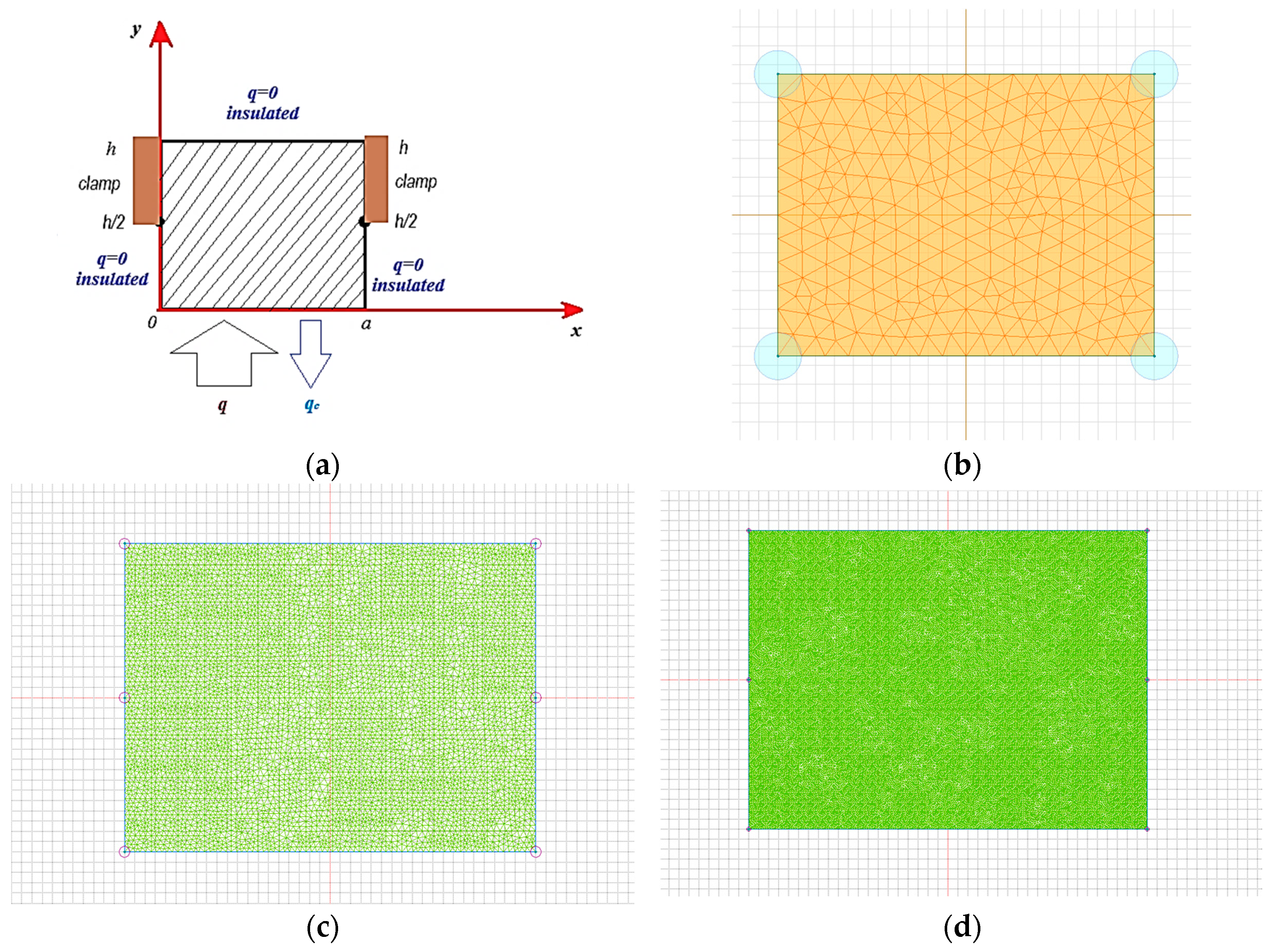
To further verify the numerical reliability of the thermal model, a mesh convergence test was conducted at the 200 V processing mode. The simulation was repeated using two progressively refined grids with approximately 6000 and 40,000 nodes.

The calculated maximum surface temperatures for these cases were 878.9 °C and 878.903 °C, respectively. Compared to the base mesh with 254 nodes (875.45 °C), the deviation between the coarsest and finest mesh solutions was only 3.45 °C, corresponding to a relative error of approximately 0.39%. These results demonstrate that the thermal field distribution stabilizes with increasing mesh resolution, and the base mesh provides sufficiently accurate results for engineering-level simulations while ensuring acceptable computational efficiency.

The data reveal a strong correlation between measured and calculated values for the 150 V and 200 V modes. However, a notable discrepancy arises at 250 V, where the numerical calculation estimates a temperature of 1127.1 °C, while the thermocouple records approximately 870 °C. This variance is primarily attributed to a technical issue involving compromised thermal contact between the thermocouple and the sample. The LOK-59 solder, used to affix the thermocouple at a 2 mm depth, has a melting point of around 900 °C. As temperatures surpass this threshold, partial melting of the solder can occur, impeding effective heat transfer between the sample and the thermocouple’s sensing element, thereby causing an underestimation of actual temperature values. Furthermore, radiative heat exchange between the sample’s heated surface and the surrounding environment becomes more significant above 1000 °C. This can induce heat redistribution and deviations from the idealized conditions assumed in the model. These factors clarify the divergence between computed and empirical data at 250 V, underscoring the necessity for meticulous interpretation of thermometry results in high-temperature electrolytic plasma hardening scenarios.

For future studies involving elevated-temperature EPH regimes, it is recommended to employ thermocouples with higher thermal stability and reduced response time, such as tungsten–rhenium or miniature fast-response sensors. Additionally, the use of high-melting-point solders (e.g., VPR-1 or VPR-11, with melting points exceeding 1000 °C) is advisable to ensure reliable thermal contact throughout the entire heating cycle. These modifications would enhance the accuracy of temperature measurements and support more robust validation of thermal models under extreme processing conditions.

To assess the thermal action efficiency across various EPT modes, the average heating rates at a 2 mm depth from the sample surface were calculated over the entire heating period. Experimentally, these rates were found to be 35.4 °C/s at 150 V, 62.5 °C/s at 200 V, and 92.9 °C/s at 250 V. Numerical estimations produced similar values of 37.9 °C/s, 67.9 °C/s, and 112.4 °C/s, respectively. These findings indicate a strong correlation between experimental results and calculations, accounting for errors introduced by the measuring system’s inertia. Notably, the local heating rates near the surface during the initial processing seconds significantly surpass these averages, potentially reaching hundreds of degrees per second, particularly at 250 V. This underscores the thermal effect’s intensity and elucidates the rapid attainment of critical temperatures in the material’s surface layers.

The average cooling rates at a depth of 2 mm following the EPD, as determined numerically, were 16.7 °C/s (150 V), 34.6 °C/s (200 V), and 59.8 °C/s (250 V). Experimentally, slightly lower values were observed at 15.0 °C/s, 30.4 °C/s, and 47.8 °C/s, respectively. This difference can be attributed to the thermocouple’s inertia and potential degradation of thermal contact at elevated temperatures. Notably, during the initial seconds after voltage termination, instantaneous cooling rates can reach hundreds of degrees per second. Such rapid thermal unloading fosters conditions conducive to martensite and bainite formation, even in low-carbon steel 20GL, particularly within the surface layers.

The elevated values obtained from the numerical calculations can be primarily attributed to inherent simplifications within the model. These simplifications pertain to the boundary conditions, specifically the assumption of a heat-insulated surface, given the substantial size of the holder. Additionally, the model does not account for the oscillatory nature of heating as a boundary condition with heat flow. For preliminary engineering assessments, such assumptions are deemed reasonable to avoid unnecessary complexity. The primary objective of this study was to investigate the feasibility of hardening low-carbon steel 20GL through electrolytic plasma treatment and to evaluate the depth of thermal influence on the samples. Future research endeavors will aim to incorporate a more comprehensive analysis of all conditions involved in the electrolytic plasma hardening of components.

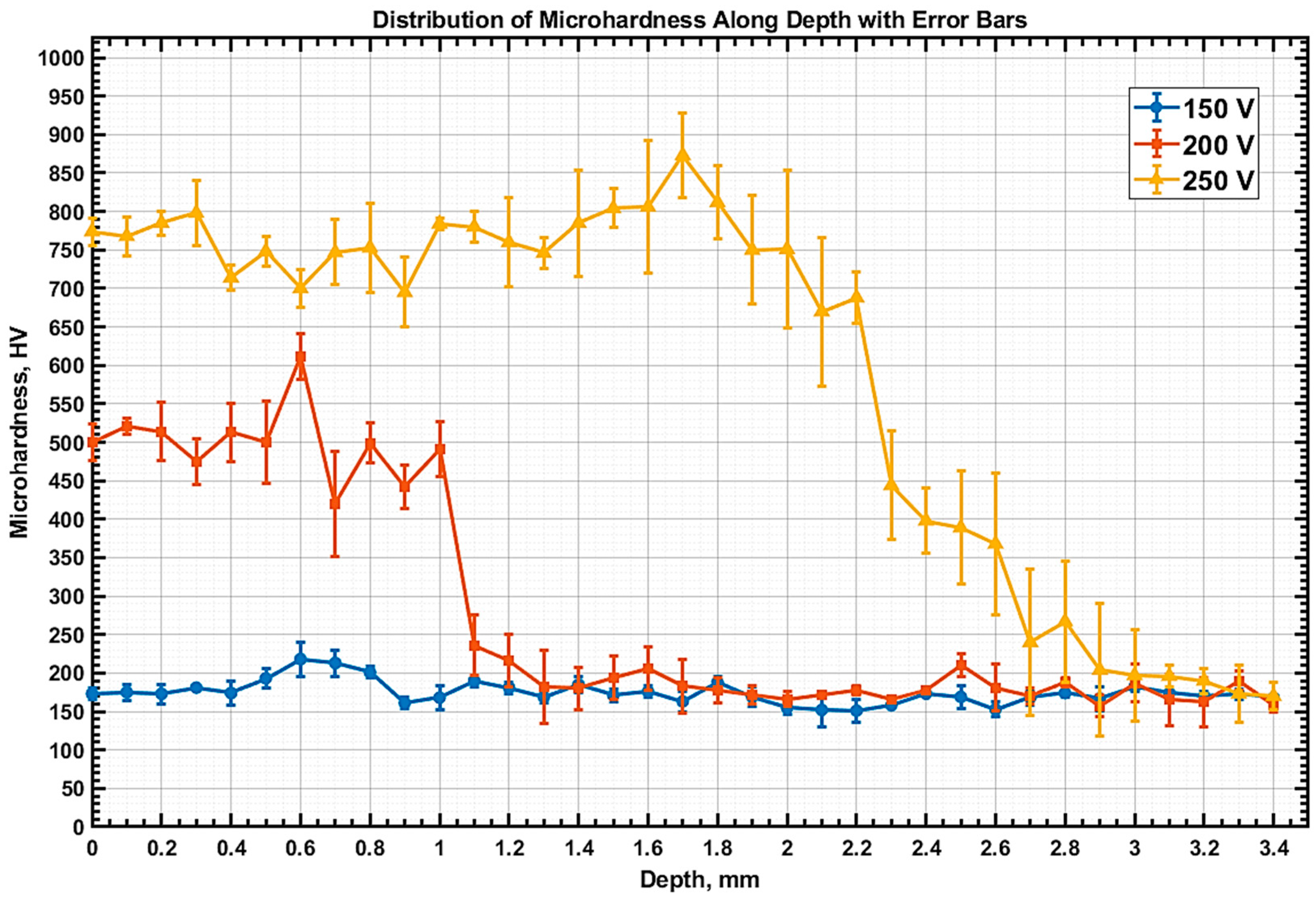
The distribution of microhardness by depth (Figure 10) clearly shows how the hardening of 20GL steel depends on the electrolytic plasma treatment mode. Initially, the samples had a microhardness of approximately 150–160 HV. The cross-section for measurement was made at a distance of approximately 5 mm from the edge of the sample. At 150 V, hardening is minimal, with a maximum hardness of about 200 HV. This aligns with the calculated temperature of less than 400 °C at a depth of 2 mm, indicating an inability to reach the critical temperature required for phase transformations. At 200 V, a notable increase in microhardness to 500 HV occurs in the surface zone, followed by a sharp decline after 1 mm of depth. Although the numerical temperature distribution predicts heating to 700–800 °C at a depth of 1–2 mm, the reduction in hardness suggests an inadequate cooling rate in these layers, which restricted the formation of bainite or martensite structures. The most substantial strengthening is observed at 250 V, where high microhardness (750–850 HV) is sustained in the zone up to approximately 2.2–2.4 mm. This aligns with calculations showing that the temperature at this depth exceeded 750 °C, and the cooling rate (>50 °C/s) was sufficient to develop a martensitic structure. Therefore, for 20GL steel, which has limited hardenability, the effective strengthening depth depends not only on the heating temperature but also on achieving critical cooling rates, especially during high-voltage EPH.

The sharp drop in hardness observed at 200 V can be explained as follows. At the end of the heating stage (t = 10 s), the surface and subsurface layers (up to ~1.5 mm) had reached temperatures in the range of 723–875 °C, sufficient for austenitization. During the subsequent 5 s cooling phase in a vigorously circulated electrolyte (at ~20 °C), a rapid temperature drop occurred. The computed cooling rate at the sample surface reached approximately 77 °C/s, gradually decreasing with depth. At depths of 1.25 mm and 1.5 mm, the cooling rate fell to around 52 °C/s and 48 °C/s, respectively—close to the critical threshold for martensitic transformation in low-carbon steels. Beyond these depths, the cooling rate continued to decline, becoming insufficient to support the formation of martensite.

This behavior aligns well with the experimentally observed hardness profile: a hardened layer of ~1.5 mm with high hardness (>300 HV), followed by a steep decrease in hardness to base values (~150 HV) corresponding to the ferrite–pearlite microstructure in the unaffected core. In this way, the interplay between two critical conditions—(1) exceeding the austenitization temperature and (2) ensuring a high enough cooling rate—explains the formation of a relatively shallow hardened layer. This confirms that the sharp drop in hardness is not an anomaly but a direct consequence of the thermal field and transformation kinetics, further validating the numerical model.

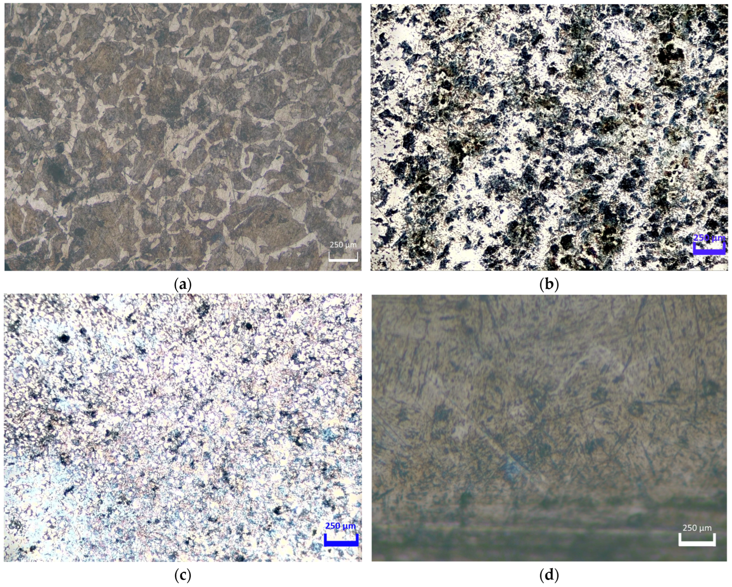
Microstructural analysis of 20GL steel samples following EPH (Figure 11) enables a visual evaluation of how different treatment modes impact surface alterations in the material. Initially, the microstructure exhibits characteristics typical of as-cast low-carbon steel, featuring a coarse-grained ferrite–pearlite morphology (Figure 11a) and a corresponding low microhardness of approximately 150 HV. After treatment at 150 V (Figure 11b), the microstructure remains largely unchanged, with only isolated regions of dispersed pearlite observed, leading to a modest increase in microhardness up to 180 HV. This suggests minimal phase transformation, consistent with the temperature profile, which indicates that heating in the surface region was insufficient to induce austenitization.

At 200 V (Figure 11c), a more noticeable alteration in the microstructure occurs, where the surface takes on a finer grain morphology. Zones of transitional bainite or incomplete martensitic transformation may also be present, correlating with a sharp increase in microhardness to 500 HV. The most substantial changes are observed at 250 V (Figure 11d), where the structure exhibits a typical martensitic morphology with an acicular texture and a maximum microhardness of approximately 800 HV. This indicates that at high voltage, the conditions necessary for complete austenitization and subsequent martensitic transformation are achieved in the surface layers, including a high temperature above 1100 °C and intensive cooling.

Therefore, the presented micrographs corroborate that the effectiveness of EPH for 20GL steel is directly contingent on achieving critical temperatures and cooling rates. The latter factor, particularly for cast steel, is decisive in the formation of a hardened structure.

4. Conclusions

This research presented a thorough investigation into the heating and hardening mechanisms of low-carbon cast 20GL steel subjected to electrolytic plasma treatment. Utilizing numerical modeling and experimental temperature field analysis, the study demonstrated that even brief exposure durations could induce substantial temperatures at depths of up to several millimeters, facilitating thermal modification of the microstructure and enhancing microhardness.

A comparison between the numerical calculation results and experimental thermometry data indicated a strong correlation at 150 and 200 V. Discrepancies observed at 250 V can be attributed to a reduction in the quality of the thermocouple’s thermal contact at temperatures exceeding 900 °C.

The analysis of microhardness distribution as a function of depth revealed a distinct correlation between hardening and localized thermal effects. The peak hardness values are observed in regions where austenitization conditions and rapid cooling rates coincide. The study determined that achieving effective hardening in 20GL cast steel necessitates cooling rates exceeding the critical threshold of approximately 50 °C/s. When rates are below this level, even upon reaching austenitization temperatures, the extent of hardening is limited, which is related to the inherent reduced hardenability of cast low-carbon steels.

Microstructural analysis confirmed the formation of martensite and bainite in the surface layers of samples processed at 200 V and 250 V, indicating the presence of high-speed quenching conditions. This demonstrates the high efficiency of EPH as a method for locally strengthening difficult-to-quench cast steels under intensive cooling conditions.

This investigation served as an initial examination of thermal phenomena during electrolytic plasma hardening for low-carbon 20GL steel, offering an initial quantitative evaluation of heat flows, heating and cooling rates, and heating depth under varying processing conditions. Future research will involve more detailed structural analyses utilizing scanning electron microscopy (SEM), electron backscatter diffraction (EBSD), and phase analysis techniques. These future investigations aim to elucidate transformation mechanisms and formulate technological recommendations for employing EPH to enhance the wear resistance and extend the service life of cast steels in practical production environments.