C Band 360° Triangular Phase Shift Detector for Precise Vertical Landing RF System

Abstract

This paper presents a novel design for precise vertical landing of drones based on the detection of three phase shifts in the range of ±180°. The design has three inputs to which the signal transmitted from an oscillator located at the landing point arrives with different delays. The circuit increases the aerial tracking volume relative to that achieved by detectors with theoretical unambiguous detection ranges of ±90°. The phase shift measurement circuit uses an analog phase detector (mixer), detecting a maximum range of ±90°and a double multiplication of the input signals, in phase and phase-shifted, without the need to fulfill the quadrature condition. The calibration procedure, phase detector curve modeling, and calculation of the input signal phase shift are significantly simplified by the use of an automatic gain control on each branch, dwhich keeps input amplitudes to the analog phase detectors constant. A simple program to determine phase shifts and guidance instructions is proposed, which could be integrated into the same flight control platform, thus avoiding the need to add additional processing components. A prototype has been manufactured in C band to explain the details of the procedure design. The circuit uses commercial circuits and microstrip technology, avoiding the crossing of lines by means of switches, which allows the design topology to be extrapolated to much higher frequencies. Calibration and measurements at 5.3 GHz show a dynamic range greater than 50 dB and a non-ambiguous detection range of ±180°. These specifications would allow one to track the drone during the landing maneuver in an inverted cone formed by a surface with an 11 m radius at 10 m high and the landing point, when 4 cm between RF inputs is considered. The errors of the phase shifts used in the landing maneuver are less than ±3°, which translates into 1.7% losses over the detector theoretical range in the worst case. The circuit has a frequency bandwidth of 4.8 GHz to 5.6 GHz, considering a 3 dB variation in the input power when the AGC is limiting the output signal to 0 dBm at the circuit reference point of each branch. In addition, the evolution of phases in the landing maneuver is shown by means of a small simulation program in which the drone trajectory is inside and outside the tracking range of ±180°.

1. Introduction

Landing is one of the most dangerous and complex maneuvers in the flight of a multirotor drone. It is usually performed in an automated way when precision in terms of location and orientation is required: battery recharging, approach to recharge sensors by induction, sampling of a specific terrain location, or simply maneuvering in an area with many obstacles [1,2]. As well as drone stabilization maneuvers, a precision landing requires a large amount of averaged telemetry data to continuously correct its position in adverse conditions: poor coverage of global/local positioning systems, rough terrain, woody vegetation, air turbulence, etc. [3,4]. Automated landing maneuvers are usually based on pattern recognition through image processing or trilateration. The latter consists in either wide coverage as Global Positioning System (GPS) or local as those based on Ultra Wide Band (UWB) communication systems.

Classic image processing systems with patterns located at the landing point [5,6,7] are sometimes combined with LEDs that provide additional information when visibility is poor [8,9]. Their main advantage is that they use a simple camera pointing to the landing point (LP) but require medium capacity memory to store the images and high computational load units [10,11,12]. Thirty frames per second camera already establishes an output data rate (ODR) of 30 Hz, i.e., a minimum time between maneuver corrections of 33 ms, which must be added to the processing and averaging time [13]. The resulting time is far from the 10 or 20 ms (100 or 50 Hz ODR) provided by drone stabilization systems and would be appropriate for a precision landing that requires compensating for turbulence generated by wind or propellers in the vicinity of the ground.

Among the automated landing systems using trilateration, those using basic GPS technology or enhanced with real-time kinematics (RTK) stand out [14,15]. However, the data is provided with approximately 1 Hz ODR and may decrease when there are obstacles around the landing point [16,17]. The positioning based on the UWB communication system has been mainly used indoors [18,19], where several nodes are configured to act as anchors listening for range requests. In this case, the drone interrogates each one of them to obtain the delays and hence the associated distances. Regardless of the distance errors with respect to the LP and ODR value that can be obtained with UWB-based systems (3.3 Hz in [20], 20 Hz in [21], or 25 Hz in [22]), the main drawback is that all these systems require units with high computational load and programs that use redundancy to improve accuracy [19,20,21,22,23,24,25,26].

Recently, a solution based on triangular phase shift detection [25] has been proposed, which significantly reduces the computations needed to obtain the correction instructions in the landing maneuver and increases the ODR to values provided by the drone stabilization systems. The radio frequency (RF) circuit allows a control based on the detection of the phase shift of three input signals coming from an oscillator located at the landing point. The system is capable of tracking in an inverted conical volume, where the vertex would be the LP, and the tracking area increases with height and decreases as frequency rises. The phase detection is performed with the AD8302 circuit, which has an integrated signal compression system, so that the analog detector or multiplier does not vary the output voltage as a function of the input voltage. However, the tracking area determined by the unambiguous phase detection range is less than the theoretical value of ±90°. The reduction in the detection range to ±80° is mainly due to mismatching and unbalancing of the RF branches of the circuit. In addition, the proposed circuit is designed at 2.5 GHz, which implies a relatively large antenna array size [27] and lacks an interference protection system [28].

Regarding phase detectors, the digitals and those that combine double multiplication are appropriate to increase the detection range and frequency. The digital ones can cover detection ranges greater than ±180° and are immune to amplitude variations in the input signal. However, the limited operating frequency of about 10 GHz is their main drawback [29,30,31], as are FPGA-based phase detectors below 1 GHz [32,33]. Another more complex measurement method, limited in frequency and occasionally used, is based on the phase variation of a reference oscillator and subtraction with each of the input signals to locate a null [34]. However, the solution requires time to sweep all phase values, so it is used when the phase does not vary rapidly.

There are other solutions with small detection range that sum the input signals (0 V output voltage when phase shift is 180°) and obtain good resolutions when the input phase shift varies ±60° over 180° of phase shift reference [35]. To change the reference value, phase shifters are introduced in one of the branches [36]. Thus, with a 180° phase shifter, it would operate around 0°. The phase detection range based on the analog phase detector can be extended to 360° by a double product in phase (I) and quadrature (Q) of the two input signals [37,38]. These circuits are integrated up to 100 GHz [39,40], but in all cases, the quadrature condition must be met, which also requires good balancing between the branches that carry the signals from the antennas (RF input) to the integrated circuit. A variant of these circuits is the phase detector with double multiplication, in phase and phase-shifted, which avoids the need to fulfill the quadrature condition [41]. This facilitates circuit design in any frequency band where multipliers (mixers) are available. However, the calibration and modeling of these detectors can become very complex, especially when the input amplitude can vary and be different at each of the input RF ports [42]. The phase shift is obtained from an interpolation process using two multidimensional matrices of calibrated data. Accuracy increases with the number of points contained in the matrices, but a powerful data processing unit is required to reduce the computing time. If the frequency increases, the synchronization requirements of the generators used to characterize the phase detector further complicate the calibration and measurement process [43]. Nevertheless, these processes are simplified if the input powers do not vary and the bandwidth is very narrow [41]. A more detailed comparative analysis of RF phase detectors can be found in [43].

In order to solve some of the limitations shown by previous designs for vertical landing of drones, we propose the design of a novel triangular phase shift detector with a range of ±180°, based on switched dual-product phase detectors with AGC. The design procedure increases the phase detection range to ±180° and, therefore, the tracking area. This allows the frequency to be increased and size of antennas to be reduced, while maintaining the tracking area similar to solutions operating at ±90°. The inclusion of the AGC simplifies the modeling of the detector curves and the circuit calibration procedure. In addition, it significantly reduces the calculations required to obtain phase shifts, allowing the use of low computing power platforms. Furthermore, a C band prototype has been manufactured to explain the details of the design procedure, and a simple landing program has been developed to show the drone guidance algorithm and detection outside the tracking area.

This paper is organized as follows: Section 2 reviews the fundamentals of precision landing by triangular phase shift detector, describes the limitations of the precision landing system with ±90° detector, and justifies the choice of using a 360° phase detector of double multiplication, in phase and phase-shifted. All the keys to the design of the C frequency band-fabricated circuit are detailed in Section 3, which includes the experimental characterization of the prototype and quantification of the phase errors. Section 4 develops the algorithm to calculate the phase and the guidance program during the landing maneuver. Next, the landing algorithm is evaluated by means of a small simulation program to assess its theoretical behavior when the drone is inside and outside the tracking range of ±180°. Finally, the results are discussed in Section 5.

2. ±90° Versus ±180° Landing System

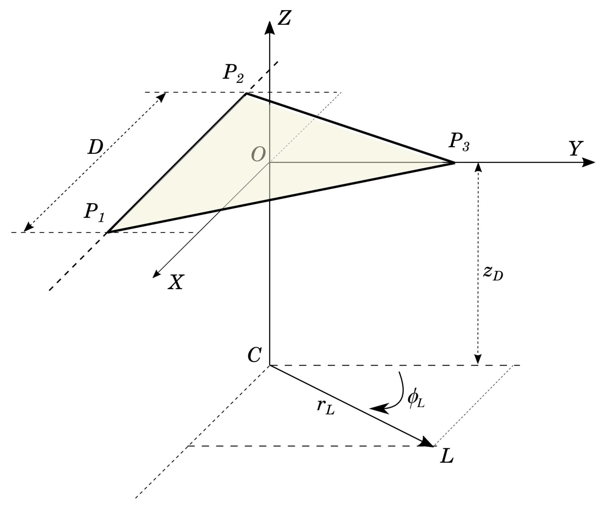
2.1. Basic Theory of Triangular Phase Shift Detector and Tracking Volume

Assuming that the LP is perpendicular to the plane formed by the receiving points (Figure 1), the equations from which the tracking zones are derived are as follows:

$$\begin{array}{ccc}\hfill \overline{O{P}_1}& =& {\displaystyle \frac{D}{2}}\widehat{x}-{\displaystyle \frac{D}{2}}tan{\displaystyle \frac{\pi }{6}}\widehat{y}\hfill \\ \hfill \overline{O{P}_2}& =& {\displaystyle \frac{-D}{2}}\widehat{x}-{\displaystyle \frac{D}{2}}tan{\displaystyle \frac{\pi }{6}}\widehat{y}\hfill \\ \hfill \overline{O{P}_3}& =& 0\widehat{x}+{\displaystyle \frac{D}{2cos(\pi /6)}}\widehat{y}\hfill \end{array}$$

(1)

$$\begin{array}{ccc}\hfill \Delta d_{ij}& =& |\overline{OL}-\overline{O{P}_i}| - {|\overline{OL}-\overline{O{P}_j}|}_{ (ij=12,23,31)}\hfill \end{array}$$

(2)

$$\begin{array}{ccc}\hfill \Delta {\theta }_{ij}& =& 2·f·\Delta d_{ij}·180/c\left[deg\right]\hfill \end{array}$$

(3)

Equation (1) gives the coordinates at which the receivers are located when they are separated by a distance of D cm, and the incenter of the triangle is at point O. The phase shifts between the received signals (Equation (3)) are determined by the distance differences between each receiving point and the LP (Equation (2)), where f is the frequency (Hz) and c is the wave travel speed (3 × ${10}^{10}$ cm/s).

As the drone moves, the distances to each of the receivers will change and, therefore, the phase shifts between them. From these, the drone will perform flight maneuvers until it reaches the LP and descends in a maneuver in which it must continuously correct its trajectory. The maximum detector phase shift determines the volume over which the drone can move (tracking volume or tracking area for a given altitude). To simplify the calculation procedure, the volume is obtained by considering that the LP (point L in Figure 1) moves in a radius $r_L$ and phase ${\varphi }_L$ when the drone varies its height $z_D$ (Figure 2). For each phase ${\varphi }_L$, the value of $r_L$ is increased until one of the phase shifts (Equation (3)) reaches the maximum value of the detector.

2.2. Triangular Phase Shift Landing System with Analog Multipliers

Phase detectors based on analog multipliers (Figure 3) have an unambiguous phase detection range of ±90° (bijective function between input phase shifts and output voltage) when the branches are well balanced ($\beta$ = 0° in Figure 3a). Otherwise, there is a reduction in the detection range directly proportional to the unbalance between branches (Figure 3b); for example, the unambiguous symmetrical range is reduced to ±(90 − $\beta$)°, ±60° in Figure 3b. That reduction in the unambiguous range results in a decrease in the tracking area in which the drone can be guided to the landing point. Figure 4a shows the tracking area for ±90° and ±60° of unambiguous phase when the drone is at 2 m height, 7 cm between antennas (D = 7 cm), and a working frequency of 2.5 GHz. The maximum distance goes from 113.5 cm to 69.7 cm, while the minimum distance goes from 94.8 cm to 59.6 cm.

2.3. Extending Phase Shift to ±180°

A 360° (±180°) phase detector allows one to increase the tracking area. Figure 4b shows the tracking area in the conditions set in Section 2.2 when the unambiguous range is ±180°. The maximum distance reaches 1338 cm, and the minimum distance increases to 332.8 cm. This means a relative increase of 3.5:1 and 11.8:1 with respect to the minimum and maximum distance for an unambiguous range of ±90°. A larger phase range translates into a larger tracking distance. If the frequency increases in the same proportion as the increase in the phase range, the tracking distance remains but allows using smaller antennas and, therefore, reducing the distance between receiving points (D). For example, Figure 5 shows the increase in tracking volume when D = 4 cm, the frequency is 5 GHz, and the phase range is +180°. Compared with Figure 2, the maximum distance at a height of 10 m increases from 569 m to 1730 m (3.0:1 distance ratio) and the minimum distance from 474 m to 1134 m (2.4:1 distance ratio). The increase in tracking distance is due to the reduction in distance D from 7 cm in Figure 2 to 4 cm in Figure 5.

In this paper, we have decided to use a 360° phase detector with double multiplication, in phase and phase-shifted (IQ-$\beta$ phase detector), because it can be easily extrapolated to other frequency ranges and technologies [41], as well as being quite immune to inter-branch unbalance. Its operation is similar to the IQ phase detectors (Figure 6a with $\beta$ = 0°), but it does not have to fulfill the quadrature condition strictly (Figure 6a with $\beta$ < 90°), which provides more flexibility in the design. Figure 6b shows the output signals of the IQ-$\beta$ phase detector that allow the phase shift to be obtained. In both cases, the output voltages of the multiplier when the input signals are in phase and quadrature (shifted) are needed to obtain the phase shift, which implies calibration and storage of the output curves for each input amplitude and frequency. In addition to all this, the IQ-$\beta$ phase detector obtains the phase difference from a somewhat more complex calculation procedure [42,43]. In simplified terms, the solution phase shift will be the one with the smallest difference between those obtained through the voltage ${V_d}_I$ in curve C.1 and ${V_d}_Q$ in curve C.2 (−100° in Figure 6b). The solution would be calculated from the voltage closest to zero volts (lower phase error versus amplitude noise) and its associated curve (circled ${V_d}_I$ in blue color).

3. Circuit Design

3.1. Theoretical Design

The main block diagram of the novel 360° triangular phase detector is detailed in Figure 7, where the initial values of the design are shown in parentheses. The design starts from the dynamic range specifications of the input signals, defined on the minimum and maximum expected signal. The dynamic range is set at 50 dB without taking into account the receiver sensitivity ($S_{min}$), since the system will operate over relatively short distances. Therefore, two voltage-controlled attenuators (HMC973) are included to ensure a range of 28 dB and insertion loss of 5 dB (from −5 dB to −33 dB at 5 GHz). The dynamic range of the variable attenuator is achieved with a voltage variation from 0 to 3.5 volts.

The next device that determines the design of the phase detector is the multiplier (mixer). The mixer selected is the MA4EX600L because it works well in the working band and is available in our laboratories. The manufacturer recommends a minimum local oscillator (OL) power level of 3 dBm [44] for it to function properly as a mixer. However, the device has been experimentally verified to provide a voltage of about 200 mVpp when the RF and OL inputs are −4 dBm and 5 GHz.

This power level is selected to obtain the rest of the power balance since it guarantees a correct operation as a phase detector. The output signal of the multiplier has polarity, so it is necessary to add an offset and amplification circuit to be able to use the analog-to-digital converter (ADC) of the Arduino Uno that supports signals between 0 and 5 V (Figure 8b). The signal is distributed between the multipliers through the power dividers (PD4859), which introduce an insertion loss of 3.5 dB. A half-dB margin is established, so the signal at the reference point (Test Port 1 in Figure 7) is 0 dBm. This power is taken as the reference signal throughout the receiver and is the measurement point for the automatic gain control (AGC). Since the slope of the variable attenuator is positive (HMC973), i.e., the greater the attenuation, the higher the control voltage, the power detector must have a positive slope. The PFC06073A directional coupler is connected just before the reference point to obtain the input signal to the AGC power detector (−10 dBm).

The power detector (ADL5906) should be set with the VSET voltage around 2.3 V, corresponding to the –10 dBm input power desired to be maintained about 5 GHz (Figure 3 in [45]). The circuit values are shown in Figure 8c, obtained from [45], as discussed below. A voltage level adjustment circuit is connected between the output of the power detector and the control input of the variable attenuators (HMC973). The input matching circuit consists of a 60.4 Ω parallel connected resistor. The CRMS capacitor value selected is 100 nF as a compromise between noise (40 mVpp on the output voltage signal) and response speed, which is determined by the rise (30 μs) and fall (1 ms) times of the signal level (Figure 50 in [45]). A response time smaller than 1 ms is more than enough, taking into account that the approach maneuver of the drone to the LP is relatively slow and, therefore, the amplitude variations in the input signal. The time could even be longer, but the noise improvement would be very small. The VTGT and VTADJ voltages are obtained from resistive voltage dividers and the reference voltage VREF (2.3 V). The estimated VTGT value recommended by the manufacturer is about 0.8 V over the entire frequency band, which represents a compromise between output voltage noise and maximizing dynamic range. The value is set by the 2.2 kΩ and 1.2 kΩ resistors. The VTADJ value improves temperature compensation and is frequency dependent. The estimated VTADJ value recommended by the manufacturer at 5 GHz is about 0.92 V, which is set by the 1 kΩ and 1.5 kΩ resistors (Table 4 in [45]).

Next, the rest of the circuits that are part of the basic detector scheme are selected (Figure 6): the hybrid circuit (C5060) and the switch (PE42553). The hybrid circuit presents a phase shift of the coupled output (Q) of +90° with respect to the direct output (I), introduces branch losses of 3.5 dB, and has a phase unbalance of 3.8° and 1 dB of amplitude. The switch is absortive and has insertion losses of 1 dB. A circuit that adjusts the levels of the control signals between the Arduino Uno (0–5 V) and the switch (0–3.3 V) is introduced (Figure 8a). A filter (DEA16537) with 1 dB losses is connected to the input of each branch.

The set of devices connected between the input and the reference point (Test Port 1) introduce a total theoretical attenuation of 18.5 dB, considering directional coupler losses negligible. Three amplifiers (SE5005L) with a typical gain of 30 dB have been distributed along each branch, resulting in a maximum gain of 71.5 dB. When the variable attenuators are at maximum attenuation (28 dB), the gain is reduced to 15.5 dB. Since the signal level at the reference point is 0 dBm, the dynamic range of the input signal varies from −71.5 dBm to −15.5 dBm.

The circuit is prepared to be controlled by an external device (control connector) or manually (DIP Switch: Dual In-line Package Switch). The switches allow the circuit branches to be turned on independently and select the direct or phase-shifted output of the hybrid circuit to generate the IQ-$\beta$ products. In addition, the control connector includes the outputs of the phase detectors (

Table 1. Control connector pin assignment: truth table for the input pins and voltages at the output pins.

	Type	Low (0 V)	High (3.3 V)
P1-S1 (Branch 1)	In	Off	On
P2-S2 (Branch 2)	In	Off	On
P3-S3 (Branch 3)	In	Off	On
P4-S4 (Switch 1)	In	Phase-shifted	In phase
P5-S5 (Switch 2)	In	Phase-shifted	In phase
P6-S6 (Switch 3)	In	Phase-shifted	In phase
P7 ($V_{d_{12}}$)	Out
P8 ($V_{d_{23}}$)	Out
P9 ($V_{d_{31}}$)	Out

).

Table 2. Truth table for IQ-$\beta$ products used to obtain the phase shifts $\Delta {\theta }_{ij}$.

Switches			Output Voltage of Phase Detector
S4	S5	S6	$\mathbf{\Delta }{\mathit{\theta }}_{\mathbf{12}}$	$\mathbf{\Delta }{\mathit{\theta }}_{\mathbf{23}}$	$\mathbf{\Delta }{\mathit{\theta }}_{\mathbf{31}}$
0	0	0	${V_{12}}_{QQ}$	${V_{23}}_{QQ}$	${V_{31}}_{QQ}$
1	0	0	${V_{12}}_{IQ}$	${V_{23}}_{QQ}$	${V_{31}}_{QI}$
0	1	1	${V_{12}}_{QI}$	${V_{23}}_{IQ}$	${V_{31}}_{QI}$
0	0	1	${V_{12}}_{QQ}$	${V_{23}}_{QI}$	${V_{31}}_{IQ}$

includes the state relationship of the switches and the phase detector output voltages (IQ-$\beta$ products). The values selected to obtain the phase shifts between the RF inputs have been highlighted in green.

3.2. Circuit Adjustments

In the first tests, oscillations in the passband occurred when each of the branches was connected independently. The unstable behavior increased when all three branches were connected. Therefore, attenuators were placed between the amplifier stages to improve stability in addition to reducing the gain of each amplifier (23 dB per amplifier) to a maximum gain of 52 dB, i.e., a theoretical dynamic range of the input signal varying from −52 dBm to 3 dBm. However, the maximum level is reduced to −2 dBm to avoid damage to the first input amplifier, leaving a dynamic range of 50 dB. This dynamic range is 20 dB higher than that achieved in [25], which uses the AD8302 circuit and had a proper performance between −10 dBm and −40 dBm. Figure 9 shows a photograph of the circuit board where the triangular layout of the RF input connectors (white lines) and the three areas containing the devices that make up each of the branches of the circuit (red lines) have been highlighted. The location of the main components of each branch is detailed in Figure 10.

3.3. Experimental Characterization

Once the generators are calibrated in the operating frequency (5.3 GHz) [42,46], the detector curves are obtained for each of the combinations in Table 2. The generators are connected to two inputs and the third one is loaded with 50 Ω. This operation is performed with the three possible combinations: 1-2, 2-3, and 3-1. In each connection, the phase of one of the reference generators is modified and the detector output data is taken. This operation is repeated to obtain the curves Q × Q (in phase) and I × Q (shifted phase). Figure 11 shows the six curves corresponding to the IQ-$\beta$ products.

The curves have a sinusoidal aspect, so a piecewise characterization is not considered [42]. Equation (4) is the function selected to model the detector behavior, and by means of a simple least squares algorithm, the values shown in

Table 3. Values of the function modeling the phase detector curves.

$\mathit{D}\mathit{C}$	A	${\mathit{d}}_{{\mathit{p}\mathit{h}\mathit{a}\mathit{s}\mathit{e}}_{\mathit{d}\mathit{e}\mathit{g}}}$	Curve	Inputs
2.3169	2.0173	243.5288	$Q\times Q$	1-2
2.3044	1.8025	127.1475	$I\times Q$	1-2
2.3161	2.0857	84.8720	$Q\times Q$	2-3
2.3444	1.8893	320.1708	$I\times Q$	2-3
2.3636	1.9995	343.6281	$Q\times Q$	3-1
2.3558	1.7404	214.9538	$I\times Q$	3-1

are obtained. Figure 12 shows the best and worst case error curves (difference between modeled equations and data), which do not exceed 0.15 V error.

$$DC+A·cos(wt+{d_{phase}}_{deg}·\pi /180)$$

(4)

However, what is important is to know how these amplitude errors are transformed into phase errors, which will be the difference between the measured and calculated values for each pair of ${V_d}_I$ and ${V_d}_Q$ values. The calculation of the phase errors is performed from the IQ-$\beta$ voltages (six voltages corresponding to ${V_d}_I$ = ${V_{ij}}_{QQ}$ and ${V_d}_Q$ = ${V_{ij}}_{IQ}$ for $i=1, 2, 3$ and $j=2, 3, 1$) and the modeled sinusoidal curves of each detector (Table 3), as indicated in Section 2.3 (Figure 6b). Figure 13 shows the phase errors for each detector, which do not exceed ±4° in any case. In fact, the phase shifts provided by curves 1-2 and 2-3, which do not exceed ±3°, can be used to obtain the third one, taking into account that the sum of the phase shifts is zero [25]. This error translates into 1.7% losses (3/180%) over the detector theoretical range in the worst case. That is, the unambiguous range of phase detection is reduced to ±177°.

The bandwidth of the circuit was obtained from the minimum input power that stabilizes the reference point power to 0 dBm (Figure 7), i.e., when the AGC is limiting the signal.

Table 4. Minimum input power versus frequency that stabilizes the reference point power to 0 dBm (Figure 7). The 3 dB bandwith extends from 4.8 GHz to 5.6 GHz.

	Frequency (GHz)
	4.7	4.8	4.9	5.0	5.1	5.2	5.3	5.4	5.5	5.6	5.7
$S_{in}$ (dBm)	−46	−49	−51	−51	−50	−52	−52	−52	−50	−50	−45

represents the measured powers for each frequency, showing that the 3 dB bandwidth extends from 4.8 GHz to 5.6 GHz.

4. Landing Algorithm and Evaluation

The landing algorithm used in [25,27] is formulated in terms of the voltages measured at the output of each of the analog phase detectors because there is a bijective relationship between phase and voltage. However, the voltages directly measured at the dual multiplier phase detector do not provide direct information to be used in the landing algorithm.

The landing algorithm is based on the offsets between the input signals to each of the three receiving points located on the drone when transmitting from the LP (Equation (3)). The objective is to locate the incenter of the drone over the LP. In that case, the distances between the LP and the vertices of the receiving triangle are identical, and hence, the three phase shifts will be zero. If the drone is considered to be at a height $z_D$ and the LP is at a distance $r_L$ and rotates around according to angle ${\varphi }_L$, the input phase shifts vary as shown in Figure 14. The crossing points between the detector curves determine the limits of each of the six sectors in which the LP can be located. Figure 14 includes the relationships between the phase shifts for the different sectors and the relative location of the drone, which will serve as the basis for performing the landing algorithm with the maneuvers that guide the drone towards the LP. Figure 15 shows the landing algorithm to be used in this case, which should be in terms of the offset between the input ports. Unlike the algorithms used in [25,27], where ±60° turns were performed to orient the drone so that the landing point was in Sector 1, this algorithm proposes to reach that situation through smaller corrections. This leads to a more realistic correction adapted to the drone dynamic movements, as is performed in the stabilization phase with pitch and roll data [47,48].

The flight maneuvering algorithm detailed in Figure 15 has been validated using a simple program. From the positioning of the drone and the LP, the three phase shifts between the RF inputs are calculated (Equation (3)). The phase shifts can exceed the range ±180°. Next, the three pairs of voltages ${V_d}_Q$ and ${V_d}_I$ are obtained using both Equation (3) and coefficients from Table 3. The new phase shifts ($\Delta {\theta }_{12}$, $\Delta {\theta }_{23}$ and $\Delta {\theta }_{31}$) are calculated from these voltages and following the procedure described in Section 2.3. This operation is going to provide an offset between ±180°. The phase shift values are used in the landing algorithm (Figure 15) to determine the maneuver to be performed. This process and the descent are performed continuously until the drone lands ($z_D$ = 0). The simulation uses 1° increments for the rotation and 1 cm for the forward/reverse. The descent increment starts at zero and increases progressively up to 1 cm when the drone is on the LP perpendicular.

Figure 16 shows the evolution of the drone in cylindrical coordinates when it starts from position {0, 0°, 500}, oriented along the positive Y axis, and the LPs are located at angles multiples of 60° about an initial reference of −35° {$490, (-35+n·60)$°, 0}. The LP locations have been selected to ensure that some of the trajectories did not reach the corresponding LP. Figure 17 shows the phase evolution in the landing maneuver when the drone reaches the LP and when it does not (LP6). In the second case, it is observed that the phase changes abruptly (green circle in Figure 17), corresponding to a situation in which the drone leaves the unambiguous zone, which is the reason why it fails to reach the LP. In the rest of the cases, the phases stay within the unambiguous range and achieve their objective. In the same figure, the evolution of the distance to the LP, measured between the incenter of the triangle of receivers in the drone and the LP, has been plotted.

5. Discussions

In this paper, a design methodology has been developed for a circuit that can function as a phase shift measurement instrument and assist in the vertical landing maneuver of a drone. The methodology has been applied to a prototype manufactured in the C band and microstrip technology. The circuit consists of three RF inputs that are combined two by two to obtain the phase shifts from the output voltages of the detectors. The transmitter is located at the landing point.

The main virtue of the designed circuit is the ability to obtain high ODR values for a given computational capacity, compared to those of imaging [5,6,7,8,9,10,11,12,13] or UWB [18,19,20,21,22,23,24,26]. The ODR will be determined mainly by the speed in obtaining the phase shifts between the input signals. The designed circuit is not as fast as that of [25] because that circuit can operate directly with voltages proportional to the ±90° phase shift. In contrast, it has a lower tracking area. However, the tracking range and ODR could be maintained using digital detectors with ±180° reaching 8 GHz, as used in the frequency synthesizer of [30]. The topology used in this paper needs to acquire two voltages to calculate the phase shift by software as in [24pablo, 25pablo, [41,42,43,49,50]]. Microstrip technology has been used, and by switching the input signals (Q and I) to the phase detector, line crossover has been avoided. This will mean dividing the ODR of [25] by at least a factor of two, while maintaining the tracking area of ±180°. However, compared to a solution using ±180° digital detectors, it allows one to extend the frequency range in an almost unlimited way, since it uses devices (Figure 7) that are commercially available in different technologies: integrated circuits, waveguides, coaxial, etc.

The topology with the three reception points on the drone allows the correction information to be available directly, saving time compared to those who obtain it on the ground and subsequently must transmit it to the drone [10,23]. In addition, the reference signal is at a single point (as are the imaging points [5,6,7,8,9,10,11,12,13]), avoiding the visibility problems that can be presented by the dispersion of several anchors in a forest area.

However, the latter are able to correct large drone displacements when close to the LP, while the inverted cone shape reduces the correction surface (unambiguous phase) as it descends towards the LP. In practice, the drone receiver system should be at a certain distance from the LP. However, considering that the diameter of the surface is approximately twice the height of the tri-receiver (Figure 5), 25 cm drone legs would provide a surface of half a meter in diameter. On the other hand, our design has the advantage that the base can be moved in pitch and roll without varying the phases on the drone inputs since the transmitter is on the LP. On the other hand, the paper design has the advantage that the base can be pitch and roll without varying the phases on the drone inputs, since the transmitter is on the LP. In any case, the key to being able to cope with a wide variety of turbulences or movements is to have circuits that can provide a high ODR, such as the one proposed in this article.

Including an AGC in the design reduces to four curves the number of minimum functions needed to characterize the circuit response. In addition, it provides a dynamic range in excess of 50 dB, without having to handle interpolation matrices as in [42] or being limited to a single power as in [41,43]. However, it will have to operate within the linear ranges of the devices, mainly the mixer (product phase detector), in order to use simple sinusoidal modeling, unlike the matrix model used in [42], which can model any type of response and operate the circuit outside the linear ranges. Despite the introduction of the AGC, calibration is necessary for each frequency to be used. First, the phase shift of each branch depends on the frequency. Second, between the AGC reference point and the detector output are the power divider and the multiplier (Figure 7), which have a different amplitude and phase response at each frequency. However, the calibration procedure is identical at all frequencies and it is sufficient to include the parameters of the sinusoidal model (Table 3).

Despite the parameters to be included in memory (Table 3) and the calculations to switch from voltages to phases, it is still a solution that can be easily integrated into piloting platforms such as Ardupilot or Pixhawk, without the need for specific processing units. This is unthinkable when using image processing [5,6,7,8,9,10,11,12,13] or UWB [18,19,20,21,22,23,24,26], where powerful processing platforms, communication ports, and memory must be used.

The proposed system presents a 1.7% reduction in phase detection over a range of ±180° (Figure 13). The percentage affects equally the tracking area for each drone height. However, it is not considered a significant loss of range that could compromise the landing maneuver. This loss is much lower than in [25,27], when the loss was 11% over ±90°. In both cases, multipliers have been used as phase detectors. However, a displacement due to unbalance between paths is transformed into a loss of the same value when a single multiplier is used (unambiguous range ±90°), while the double multiplication procedure compensates this displacement and reduces it to 0°, i.e., the all range ±180° is available. In the article circuit, the loss of range is confined to the lack of precision in the curve modeling the detector response (Equation (4) and Figure 12), i.e., it derives from the fact that the multiplier does not have a purely sinusoidal phase response.

A simple program has been developed to show the drone guidance algorithm and the phasing behavior in the drone descent. The system with phase range ±90° must detect the proximity to the ends to determine that it is not in ambiguous area [25,27]. This is an effective reduction in the useful range. However, the topology used allows detecting the instant at which it leaves the unambiguous zone from an abrupt change in any of the phase shifts (Figure 17). If this situation occurs, the drone must undo the maneuver and return to the unambiguous zone, unlike systems based on image processing [5,6,7,8,9,10,11,12,13] or UWB [18,19,20,21,22,23,24,26], where there is no concept of ambiguous zone and they do not have this limitation.

6. Conclusions

In this paper, a novel circuit for accurate vertical landing of drones based on a triple phase detection in the range of ±180° has been presented.

• The design has been realized with a double multiplication phase detector, in phase and phase-shifted, which facilitates the design because it allows an unbalancing of the different branches without loss of detection range. The increase in the phase detection range up to ±180° transforms into a directly proportional increase in the tracking area. An analysis of the tracking volumes (inverted cones) has been performed comparing different frequencies, distances between RF inputs, and phase detection ranges (±180° and ±90°).
• The results with ±180° show the possibility of increasing the working frequency and reducing the size of the antennas, while maintaining the tracking area of systems operating at ±90°. Compared to previous designs that have used this technique, an AGC has been included that substantially simplifies the calibration and modeling of the curves of this type of detector and, therefore, the algorithm to determine the phase shift from the voltages measured at the output of the multiplier. This makes possible its integration in a simple control circuit board or as part of the flight control system.
• A simple program is proposed that implements the guidance instructions from the calculated phase shifts, which could be integrated into the same flight control platform, thus avoiding the need to add additional processing and memory components.
• A prototype has been manufactured with commercial circuits and microstrip technology that operates in the C frequency band, avoiding the crossing of lines by means of switches. In this work, the calibration and characterization process has been performed at 5.3 GHz. The measurements show a dynamic range of more than 50 dB and an unambiguous detection range of ±177°, taking into account the uncertainty produced by the phase error of ±3°. The tracking area shows a considerable increase with respect to previous developments that have a theoretical phase shift of ±90°. As shown, it changes from an area of approximately 1 m radius to 3.3 m radius when the inputs are at D = 7 cm, the frequency is 2.5 GHz, and the drone is at 2 m height (Figure 4).
• Finally, a simulation program has been developed to visualize the drone trajectories and phase evolution. Different situations have been analyzed in which the drone stays inside the tracking zone (phase shifts lower than ±180°) and achieves a successful landing or goes out of it (phase shifts higher than ±180°) and lands at any wrong location.

References

1. Woo, C.; Kang, S.; Ko, H.; Song, H.; Kwon, J.O. Auto charging platform and algorithms for long-distance flight of drones. In Proceedings of the 2017 IEEE International Conference on Consumer Electronics (ICCE), Las Vegas, NV, USA, 8–10 January 2017; pp. 186–187. [Google Scholar] [CrossRef]
2. Basha, E.; Eiskamp, M.; Johnson, J.; Detweiler, C. UAV Recharging Opportunities and Policies for Sensor Networks. Int. J. Distrib. Sens. Netw. 2015, 11, 824260. [Google Scholar] [CrossRef]
3. Gautam, A.; Sujit, P.B.; Saripalli, S. A survey of autonomous landing techniques for UAVs. In Proceedings of the 2014 International Conference on Unmanned Aircraft Systems (ICUAS), Orlando, FL, USA, 27–30 May 2014; pp. 1210–1218. [Google Scholar] [CrossRef]
4. Shakhatreh, H.; Sawalmeh, A.H.; Al-Fuqaha, A.; Dou, Z.; Almaita, E.; Khalil, I.; Othman, N.S.; Khreishah, A.; Guizani, M. Unmanned Aerial Vehicles (UAVs): A Survey on Civil Applications and Key Research Challenges. IEEE Access 2019, 7, 48572–48634. [Google Scholar] [CrossRef]
5. Patruno, C.; Nitti, M.; Petitti, A.; Stella, E.; D’Orazio, T. A Vision-Based Approach for Unmanned Aerial Vehicle Landing. J. Intell. Robot. Syst. 2019, 95, 645–664. [Google Scholar] [CrossRef]
6. Pluckter, K.; Scherer, S. Precision UAV Landing in Unstructured Environments. In Proceedings of the International Symposium on Experimental Robotics; Springer: Berlin/Heidelberg, Germany, 2018; pp. 177–187. [Google Scholar]
7. Salagame, A.; Govindraj, S.; Omkar, S. Precision Landing of a UAV on a Moving Platform for Outdoor Applications. arXiv 2022, arXiv:2209.14436. [Google Scholar] [CrossRef]
8. Janousek, J.; Marcon, P. Precision landing options in unmanned aerial vehicles. In Proceedings of the 2018 International Interdisciplinary PhD Workshop (IIPhDW), Świnoujście, Poland, 9–12 May 2018; IEEE: Piscataway, NJ, USA; pp. 58–60. [Google Scholar]
9. Badakis, G.; Koutsoubelias, M.; Lalis, S. Robust precision landing for autonomous drones combining vision-based and infrared sensors. In Proceedings of the 2021 IEEE Sensors Applications Symposium (SAS), Sundsvall, Sweden, 23–25 August 2021; IEEE: Piscataway, NJ, USA; pp. 1–6. [Google Scholar]
10. Mu, L.; Li, Q.; Wang, B.; Zhang, Y.; Feng, N.; Xue, X.; Sun, W. A vision-based autonomous landing guidance strategy for a micro-UAV by the modified camera view. Drones 2023, 7, 400. [Google Scholar] [CrossRef]
11. Liu, X.; Xue, W.; Xu, X.; Zhao, M.; Qin, B. Research on unmanned aerial vehicle (UAV) visual landing guidance and positioning algorithms. Drones 2024, 8, 257. [Google Scholar] [CrossRef]
12. García-Pulido, J.A.; Pajares, G.; Dormido, S. UAV landing platform recognition using cognitive computation combining geometric analysis and computer vision techniques. Cogn. Comput. 2023, 15, 392–412. [Google Scholar] [CrossRef]
13. Moreira, M.; Azevedo, F.; Ferreira, A.; Pedro, D.; Matos-Carvalho, J.; Ramos, Á.; Loureiro, R.; Campos, L. Precision Landing for Low-Maintenance Remote Operations with UAVs. Drones 2021, 5, 103. [Google Scholar] [CrossRef]
14. Supej, M.; Čuk, I. Comparison of Global Navigation Satellite System Devices on Speed Tracking in Road (Tran)SPORT Applications. Sensors 2014, 14, 23490–23508. [Google Scholar] [CrossRef] [PubMed]
15. Koo, G.; Kim, K.; Chung, J.Y.; Choi, J.; Kwon, N.Y.; Kang, D.Y.; Sohn, H. Development of a high precision displacement measurement system by fusing a low cost RTK-GPS sensor and a force feedback accelerometer for infrastructure monitoring. Sensors 2017, 17, 2745. [Google Scholar] [CrossRef] [PubMed]
16. Meng, Y.S.; Lee, Y.H.; Ng, B.C. Study of Propagation Loss Prediction in Forest Environment. Prog. Electromagn. Res. B 2009, 17, 117–133. [Google Scholar] [CrossRef]
17. Dyukov, A. Mask Angle Effects on GNSS Speed Validity in Multipath and Tree Foliage Environments. Asian J. Appl. Sci. 2016, 4, 309–321. [Google Scholar]
18. Tiemann, J.; Schweikowski, F.; Wietfeld, C. Design of an UWB indoor-positioning system for UAV navigation in GNSS-denied environments. In Proceedings of the 2015 International Conference on Indoor Positioning and Indoor Navigation (IPIN), Banff, AB, Canada, 13–16 October 2015; IEEE: Piscataway, NJ, USA; pp. 1–7. [Google Scholar]
19. Benini, A.; Mancini, A.; Longhi, S. An IMU/UWB/vision-based extended kalman filter for mini-UAV localization in indoor environment using 802.15.4a wireless sensor network. J. Intell. Robot. Syst. 2013, 70, 461–476. [Google Scholar] [CrossRef]
20. Queralta, J.P.; Almansa, C.M.; Schiano, F.; Floreano, D.; Westerlund, T. UWB-based system for UAV localization in GNSS-denied environments: Characterization and dataset. In Proceedings of the 2020 IEEE/RSJ International Conference on Intelligent Robots and Systems (IROS), Las Vegas, NV, USA, 24 October 2020–24 January 2021; IEEE: Piscataway, NJ, USA; pp. 4521–4528. [Google Scholar]
21. Zeng, Q.; Jin, Y.; Yu, H.; You, X. A UAV localization system based on double UWB tags and IMU for landing platform. IEEE Sens. J. 2023, 23, 10100–10108. [Google Scholar] [CrossRef]
22. Ochoa-de Eribe-Landaberea, A.; Zamora-Cadenas, L.; Peñagaricano-Muñoa, O.; Velez, I. UWB and IMU-based UAV’s assistance system for autonomous landing on a platform. Sensors 2022, 22, 2347. [Google Scholar] [CrossRef] [PubMed]
23. Kownacki, C.; Ambroziak, L.; Ciezkowski, M.; Wolniakowski, A.; Romaniuk, S.; Bozko, A.; Oldziej, D. Precision landing tests of tethered multicopter and VTOL UAV on moving landing pad on a lake. Sensors 2023, 23, 2016. [Google Scholar] [CrossRef] [PubMed]
24. Guo, K.; Qiu, Z.; Miao, C.; Zaini, A.H.; Chen, C.L.; Meng, W.; Xie, L. Ultra-wideband-based localization for quadcopter navigation. Unmanned Syst. 2016, 4, 23–34. [Google Scholar] [CrossRef]
25. Araña-Pulido, V.; Jiménez-Yguácel, E.; Cabrera-Almeida, F.; Quintana-Morales, P. Triangular Phase Shift Detector for Drone Precise Vertical Landing RF Systems. IEEE Trans. Instrum. Meas. 2021, 70, 8501808. [Google Scholar] [CrossRef]
26. Lo, T.Y.; Chang, J.Y.; Wei, T.Z.; Chen, P.Y.; Huang, S.P.; Tsai, W.T.; Liou, C.Y.; Lin, C.C.; Mao, S.G. GPS-free wireless precise positioning system for automatic flying and landing application of shipborne unmanned aerial vehicle. Sensors 2024, 24, 550. [Google Scholar] [CrossRef] [PubMed]
27. Araña-Pulido, V.; Jiménez-Yguácel, E.; Cabrera-Almeida, F.; Quintana-Morales, P. Antenna system for trilateral drone precise vertical landing. IEEE Trans. Instrum. Meas. 2022, 71, 3000508. [Google Scholar] [CrossRef]
28. Sathaye, H.; Schepers, D.; Ranganathan, A.; Noubir, G. Wireless attacks on aircraft instrument landing systems. In Proceedings of the 28th USENIX Security Symposium (USENIX Security 19), Miami, FL, USA, 15–17 May 2019; pp. 357–372. [Google Scholar]
29. Rezaeian, A.; Ardeshir, G.; Gholami, M. A low-power and high-frequency phase frequency detector for a 3.33-GHz delay locked loop. Circuits Syst. Signal Process. 2020, 39, 1735–1750. [Google Scholar] [CrossRef]
30. Microsemi. 8 GHz Phase Frequency Detector IC with Dual 40 GHz Prescalers. Available online: http://www.microsemi.com (accessed on 21 July 2025).
31. Sofimowloodi, S.; Razaghian, F.; Gholami, M. Low-power high-frequency phase frequency detector for minimal blind-zone phase-locked loops. Circuits Syst. Signal Process. 2019, 38, 498–511. [Google Scholar] [CrossRef]
32. Zhang, M.; Wang, H.; Qin, H.; Zhao, W.; Liu, Y. Phase Difference Measurement Method Based on Progressive Phase Shift. Electronics 2018, 7, 86. [Google Scholar] [CrossRef]
33. Vandenbussche, J.; Lee, P.; Peuteman, J. On the Accuracy of Digital Phase Sensitive Detectors Implemented in FPGA Technology. IEEE Trans. Instrum. Meas. 2014, 63, 1926–1936. [Google Scholar] [CrossRef]
34. Bertotti, F.L.; Hara, M.S.; Abatti, P.J. A simple method to measure phase difference between sinusoidal signals. Rev. Sci. Instruments 2010, 81, 115106. [Google Scholar] [CrossRef] [PubMed]
35. Han, J.; Ding, D. Design and Analysis of a Hybrid-Type RF MEMS Phase Detector in X-Band. Micromachines 2022, 13, 786. [Google Scholar] [CrossRef] [PubMed]
36. Widarta, A. Null Technique for Precision RF Phase Shift Measurements. IEEE Trans. Instrum. Meas. 2019, 68, 1840–1843. [Google Scholar] [CrossRef]
37. Mlynek, A.; Faugel, H.; Eixenberger, H.; Pautasso, G.; Sellmair, G. A simple and versatile phase detector for heterodyne interferometers. Rev. Sci. Instruments 2017, 88, 023504. [Google Scholar] [CrossRef] [PubMed]
38. Verhaevert, J.; Van Torre, P. A low-cost vector network analyzer: Design and realization. In Proceedings of the Loughborough Antennas & Propagation Conference (LAPC 2017), Loughborough, UK, 13–14 November 2017; pp. 1–5. [Google Scholar] [CrossRef]
39. ADMV1014. 24 GHz to 44 GHzWideband Microwave Downconverter. Analog Devices 2018. Available online: https://www.analog.com/media/en/technical-documentation/data-sheets/admv1014.pdf (accessed on 21 July 2025).
40. Abbasi, M.; Carpenter, S.; Zirath, H.; Dielacher, F. A 80–95 GHz direct quadrature modulator in SiGe technology. In Proceedings of the 2014 IEEE 14th Topical Meeting on Silicon Monolithic Integrated Circuits in RF Systems, Newport Beach, CA, USA, 19–23 January 2014; IEEE: Piscataway, NJ, USA; pp. 56–58. [Google Scholar] [CrossRef]
41. Pérez, B.; Pulido, V.A.; Perez-Mato, J.; Cabrera, F. 360° phase detector cell for measurement systems based on switched dual multipliers. IEEE Microw. Wirel. Compon. Lett. 2017, 27, 503–505. [Google Scholar] [CrossRef]
42. Pérez-Díaz, B.; Araña-Pulido, V.; Cabrera-Almeida, F.; Dorta-Naranjo, B.P. Phase shift and amplitude array measurement system based on 360° switched dual multiplier phase detector. IEEE Trans. Instrum. Meas. 2021, 70, 8005411. [Google Scholar] [CrossRef]
43. Dorta-Naranjo, B.P.; Araña-Pulido, V.; Cabrera-Almeida, F.; Jiménez-Yguácel, E. A 2–18 GHz 360° Phase Detector based on Switched Dual Multipliers and Fixed Delay Lines. IEEE Trans. Instrum. Meas. 2025, 74, 8501010. [Google Scholar] [CrossRef]
44. MA4EX600L. Silicon Double Balanced HMICTM Mixer 4.2–6.0 GHz. Macom 2023. Available online: https://cdn.macom.com/datasheets/MA4EX600L1-1225.pdf (accessed on 21 July 2025).
45. ADL5906. 10 MHz to 10 GHz 67 dB TruPwr Detector. Analog Devices 2023. Available online: https://www.analog.com/media/en/technical-documentation/data-sheets/adl5906.pdf (accessed on 21 July 2025).
46. Umpierrez, P.; Arana, V.; Ramirez, F. Experimental Characterization of Oscillator Circuits for Reduced-Order Models. IEEE Trans. Microw. Theory Tech. 2012, 60, 3527–3541. [Google Scholar] [CrossRef]
47. Höflinger, F.; Müller, J.; Törk, M.; Reindl, L.; Burgard, W. A wireless micro inertial measurement unit (IMU). In Proceedings of the 2012 IEEE International Instrumentation and Measurement Technology Conference Proceedings, Graz, Austria, 13–16 May 2012; pp. 2578–2583. [Google Scholar] [CrossRef]
48. García, J.; Molina, J.M.; Trincado, J.; Sánchez, J. Analysis of sensor data and estimation output with configurable UAV platforms. In Proceedings of the Sensor Data Fusion: Trends, Solutions, Applications (SDF), Bonn, Germany, 10–12 October 2017; pp. 1–6. [Google Scholar] [CrossRef]
49. Varavin, A.; Ermak, G.; Vasiliev, A.; Fateev, A.; Varavin, N.; Zacek, F.; Zajac, J. Three-channel phase meters based on the AD8302 and field programmable gate arrays for heterodyne millimeter wave interferometer. Telecommun. Radio Eng. 2016, 75, 1009–1025. [Google Scholar] [CrossRef]
50. Philippe, B.; Reynaert, P. A Quadrature Phase Detector in 28nm CMOS for Differential mm-Wave Sensing Applications Using Dielectric Waveguides. In Proceedings of the IEEE 44th European Solid State Circuits Conference (ESSCIRC) (ESSCIRC), Dresden, Germany, 3–6 September 2018; pp. 114–117. [Google Scholar] [CrossRef]
Figure 1. Coordinate system of the drone reception points and LP.
Applsci 15 08236 g001
Figure 2. (a) Tracking volume (inverted cone) when the phase detector has an unambiguous detection range of ±90°, D = 7 cm at 2.5 GHz. (b) Top view.
Applsci 15 08236 g002
Figure 3. (a) Multiplier as analog phase detector and multiplier output voltage. (b) Non-ambiguous symmetric range when the phase shift between branches is 90° ( β = 0°) and 90–30° ( β = 30°).
Applsci 15 08236 g003
Figure 4. Comparison of coverage areas for z D = 200 cm, f = 2.5 GHz, and D = 7 cm when the unambiguous area is (a) ±60°, ±90° and (b) ±180°.
Applsci 15 08236 g004
Figure 5. (a) Tracking inverted cone for D = 4 cm at 5 GHz and unambiguous phase range of ±180°. (b) Top view.
Applsci 15 08236 g005
Figure 6. (a) Simplified schematic of the IQ and IQ- β phase detector. (b) Output voltages for the product I (switch = 1) and Q (switch = 2) for the IQ- β modulator.
Applsci 15 08236 g006
Figure 7. Simplified schematic of the novel 360° triangular phase detector. In parentheses are the final values after adjustments.
Applsci 15 08236 g007
Figure 8. Auxiliary circuits. (a) Voltage converter circuit of the Arduino Uno control signal from 0–5 V to 0–3 V (control voltage of the PE42553 switch). (b) DC offset and gain of the multiplier output voltage, from ±100 mVpp to 0–5 V. (c) Schematic of the ADL5906 power detector that operates as part of the AGC.
Applsci 15 08236 g008
Figure 9. Photograph of the fabricated circuit showing the symmetry of each of the three RF branches.
Applsci 15 08236 g009
Figure 10. Detail photograph of one of the circuit branches, including the location of the most significant RF components.
Applsci 15 08236 g010
Figure 11. IQ- β data curves for each of the three detectors at 5.3 GHz, according to the different switch positions detailed in Table 2.
Applsci 15 08236 g011
Figure 12. Amplitude errors in the modeled detector curves at 5.3 GHz. (a) Best case corresponding to the I × Q curve and inputs 2-3. (b) Worst case corresponding to the I × Q curve and inputs 3-1.
Applsci 15 08236 g012
Figure 13. Phase errors calculated from the detector curve models and the original data used for modeling at 5.3 GHz.
Applsci 15 08236 g013
Figure 14. Phase shifts between RF ( Δ θ i j ) inputs when the LP is moved around the drone ( ϕ L ). The figure includes the relationships between the phase shifts associated with each of the 6 sectors that determine the relative location of the LP.
Applsci 15 08236 g014
Figure 15. Landing algorithm based on the phase shift ratios detailed in Figure 14 ( Δ θ 12 , Δ θ 23 , and Δ θ 31 ), indicating the movements to be performed by the drone.
Applsci 15 08236 g015
Figure 16. Three-dimensional and top view of several landing maneuvers at 5.4 GHz and D = 4 cm. Trajectories when the drone is oriented along the positive Y axis and starts from the position {0, 0°, 500}. The landing points are located at {490, (−35 + n·60)°, 0}. The original (×mark) and final (dot mark) LP have been highlighted in green when the drone has left the unambiguous zone (Figure 17).
Applsci 15 08236 g016
Figure 17. Input phase shifts and distance to LP when the drone reaches the LP (dashed lines and LP1 in Figure 16) and when it does not (solid line and LP6 in Figure 16). The green circle highlights the moment of the abrupt phase change, from 180° to −180°, to the drone leaving the tracking area.
Applsci 15 08236 g017