Advancing Knowledge on Machine Learning Algorithms for Predicting Childhood Vaccination Defaulters in Ghana: A Comparative Performance Analysis

Featured Application

This study demonstrates how machine learning can be used to efficiently predict children at risk of defaulting from vaccination schedules within a low-resource environment. The incorporation of vaccination timing windows and birth seasonality features offers novel dimensions for integrating temporal information into predictive models for vaccination uptake assessment. Policymakers and program managers in Ghana can leverage these models and features in data-driven strategies to mitigate barriers to timely vaccine uptake in the specified context. Beyond Ghana, the modelling approaches used are adaptable to other similar settings where data are available.

Abstract

High rates of childhood vaccination defaulting remain a significant barrier to achieving full vaccination coverage in sub-Saharan Africa, contributing to preventable morbidity and mortality. This study evaluated the utility of machine learning algorithms for predicting childhood vaccination defaulters in Ghana, addressing the limitations of traditional statistical methods when handling complex, high-dimensional health data. Using a merged dataset from two malaria vaccine pilot surveys, we engineered novel temporal features, including vaccination timing windows and birth seasonality. Six algorithms, namely logistic regression, support vector machine, random forest, gradient boosting machine, extreme gradient boosting, and artificial neural networks, were compared. Models were trained and validated on both original and synthetically balanced and augmented data. The results showed higher performance across the ensemble tree classifiers. The random forest and extreme gradient boosting models reported the highest F1 scores (0.92) and AUCs (0.95) on augmented unseen data. The key predictors identified include timely receipt of birth and week six vaccines, the child’s age, household wealth index, and maternal education. The findings demonstrate that robust machine learning frameworks, combined with temporal and contextual feature engineering, can improve defaulter risk prediction accuracy. Integrating such models into routine immunization programs could enable data-driven targeting of high-risk groups, supporting policymakers in strategies to close vaccination coverage gaps.

1. Introduction

Ongoing research has accentuated the significant rates of infant mortality due to vaccine-preventable diseases in low- and middle-income countries (LMICs). In sub-Saharan Africa, estimates indicate that these conditions result in approximately one million infant deaths annually [1]. As a result, reducing infant mortality associated with vaccine preventable diseases is a public health priority for many sub-Saharan African countries, where the burden is highest [2]. An aspect of high research interest is the issue of vaccination defaulting, where some children fail to complete the full vaccination schedule [3]. Defaulting can leave children vulnerable to diseases and undermine efforts to inhibit the spread of vaccine-preventable diseases, which in turn undermines mortality reduction. Common predictors of childhood vaccination defaulters are well documented in the literature [4,5,6], which include maternal literacy, household wealth, geographic disparities, and healthcare access. It is also understood that the relevance and weight of these predictors vary across populations. For example, Abateman and colleagues [7] identified maternal education level, type of community settlement, and the mother’s knowledge of childhood vaccination benefits as the most important determinants of vaccination defaulting in Ethiopia, while [8] identified place of residence, delivery location, and ANC visits as the key predictors of vaccination defaulter risk in Mali.

The task of identifying the predictors of a health outcome invariably requires the use of efficient analytical methods to assess complex population structures, health behaviour patterns, social networks, temporal events, and locational factors. While traditional statistical approaches remain valuable, they are often characterised by rigid assumptions [9] which tend to impose limitations on the extent to which they can adapt to non-linear, high-dimensional data. The new paradigm of machine learning tends to offer adaptive techniques with less rigid assumptions in handling large-scale variables [10]. Machine learning techniques provide efficient ways of using computational methods to analyse larger datasets, also with minimal human intervention during the process [11]. A wide range of machine learning techniques exist, spanning decision trees [12,13], ensemble classifiers [12,13,14], support vector machines [12], neural networks [8,14], and deep learning models [15]. These techniques are already highly valued in the field of clinical diagnostics [16]. There is also significant evidence on the contributions these novel techniques are making to improve the planning and impact of public health [17,18], especially in low-resource settings.

Increased interest in the use of machine learning models for the analysis of childhood vaccination defaulter risk predictors within resource-constrained environments is evidenced in existing studies [13,14]. Yet applications so far have adopted basic socio-demographic representations. By relying on such basic representations, a large amount of valuable information embedded within complex demographic, socio-economic, and environmental data is wasted, effecting our capability to improve the performance of learning models. One important aspect that has been underexamined in machine learning studies within the sub-Saharan African context is temporal events. For instance, the order of vaccination, as well as the time interval between them, often carries complex information that may be crucial for predicting defaulter risk [19]. At the same time, many LMICs, particularly within the sub-Saharan African region, experience multiple climatic patterns with ecological zonal variations [20,21], which could have important implications for healthcare access and delivery in underserved areas [22]. These temporal characteristics, however, are highly sensitive to inaccuracies and can produce extreme or inconsistent results if timestamps are modified. In many LMIC settings where logistical constraints result in less efficient documentation, these temporal measurements are frequently recorded with considerable noise. Therefore, using these features in machine learning models requires careful standardised, which can be tedious and time-consuming.

In Ghana, very little effort has been made to exploit machine learning techniques for childhood vaccination defaulter risk analysis. Current methods are predominantly statistical [23,24]. One of the few attempts is seen in the work of Bediako and colleagues [25], where the random forest classifier was evaluated with other statistical methods to analyse predictors of vaccination default among 600 children. In their study, the statistical techniques used provided the best prediction results, while the ensemble learning algorithm underperformed. Indeed, the malaria vaccine had been newly introduced, and so the difficulty in obtaining sufficiently large data for machine learning-based analysis would not be unusual, which could have also accounted for the relatively low depth of analysis. Meanwhile, the impact of limited data on the effectiveness of such advanced analytical techniques has been mentioned by Muhoza and colleagues [26]. In effect, a more thorough study into how machine learning methods could be leveraged for analysing childhood vaccination defaulter risk predictors in Ghana is lacking. We take this opportunity to bridge this gap through a more rigorous comparison of statistical and machine learning methods on a relatively larger dataset created by merging data from multiple surveys. We also evaluate the relevance of new predictors from temporal data, specifically the timing of vaccination and birth, in predicting childhood vaccination default.

2. Materials and Methods

The datasets for this study were obtained from a malaria vaccine pilot evaluation project (MVPE) conducted within 66 districts across three administrative regions in Ghana between April 2019 and April 2024 [27,28]. Records of children aged 4 to 48 months were extracted from a baseline and an endline cross-sectional survey. Both surveys employed identical instruments, eligibility criteria, and field data collection procedures. Moreover, there were no major changes in vaccination policy or service delivery context in Ghana, supporting their homogeneity and suitability for combined analysis. Several features were extracted from the survey datasets, which included both child and caregiver demographics, household asset ownership data, and vaccination data. In this study, considerable time and effort was spent on data preprocessing, which is often the case for studies involving the use of machine learning models [29,30,31,32]. Preprocessing tasks involved the resolution of missing values, data anomalies, and outliers due to transcription problems. Another important task performed was to standardise categorical data into binary vectors of 0 and 1. To achieve this, the one-hot encoding technique [33] was mainly used. As a result, multi-categorical features such as the mother’s education level and the mother’s occupation increased data dimensionality. To reduce data dimensionality [34], we applied the principal component analysis (PCA) technique [35]. The top 9 components, capturing 53% of the total variance, were retained. These components were then used to derive a single-point wealth index feature.

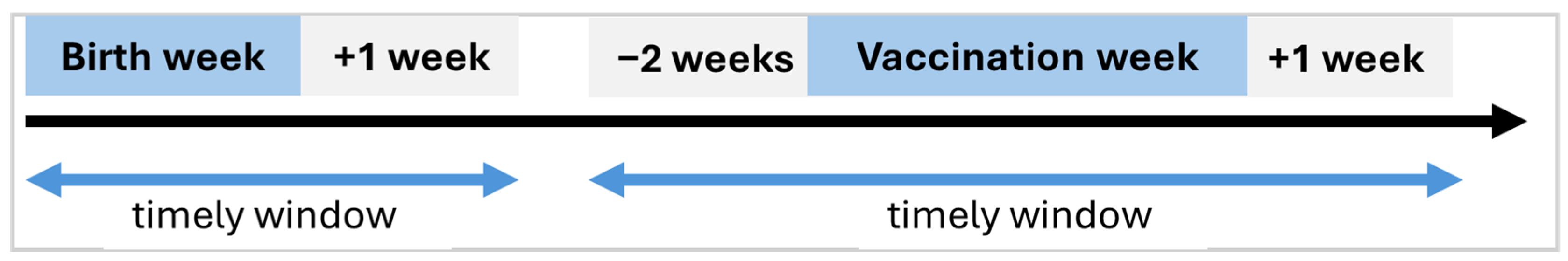
New features, including the child’s birth and timing of vaccination, were systematically engineered for modelling. With respect to vaccination timing windows, our assumptions were guided by principles used by Adetifa and colleagues [19]. We defined timelines of a vaccine schedule within the threshold of one month, with an offset of two weeks before and after the target week of schedule (Figure 1).

Table A1. The vaccination window computation for each schedule used in this study.

SCHEDULE	VACCINE(S)	WINDOW
At Birth	BCG	Week 0–Week 2
	OPV0
	HEPB
6 Weeks	PENTA1	Week 4–Week 7
	OPV1
	PCV1
	ROTA1
10 Weeks	PENTA2	Week 8–Week 11
	OPV2
	PCV2
	ROTA2
14 Weeks	PENTA3	Week 12–Week 15
	OPV3
	PCV3
	IPV
6 Months	VITA	Week 22–Week 25
	RTSS1
7 Months	RTSS	Week 26–Week 29
9 Months	MEAS1	Week 34–Week 37
	YF
	RTSS3
12 Months	MENGA	Week 46–Week 49
18 Months	MEAS2	Week 70–Week 73
	RTSS4

showing the vaccination window computation for each schedule used in this study is presented in Appendix A.

The computational logic used implies that the birth dose of the Oral Polio Vaccine (OPV0) administered beyond two weeks after birth is considered out of the timely window, while the first dose (OPV1) administered 4 to 8 weeks after birth is considered on time. Due to possible variations in the antigen-specific dates within a given schedule, the overall vaccination date for the schedule was estimated as the mean of the recorded antigen-specific dates. This derived date was then used to compute the number of days the child deviated from the recommended on-time window for that vaccination schedule. Denoting a vaccination schedule $\left(s\right)$ consisting of $\left(n\right)$ antigens, each with an associated actual vaccination date $\left\{d_1, d_2, \dots , d_n\right\}$, we modelled the derived actual vaccination date for the schedule $A_s$ as follows:

$$A_s={\displaystyle \frac{1}{n}}\sum _{i=1}^n{d}_i$$

where the actual date of vaccination for the schedule is computed as the average of the recorded antigen dates. Using the abovementioned time definitions and assumptions, two concepts were introduced to capture the timeliness of vaccine delivery at each schedule: on-time vaccination (OV) and vaccination deviation (VD). OV basically indicates whether the child received timely vaccination, while DV indicates early and late deviations from OV. The feature OV was represented as a binary vector (1 = within window, 0 = out of window) based on the upper and lower bound of each vaccination schedule. Mathematically, a given schedule ($i$) was modelled as follows:

$${OV}_i=\left\{\begin{array}{c} 1, if L_i \le A_i \le U_i\\ 0, otherwise\end{array}\right.$$

where $A_i$ represents the actual date of vaccination for schedule ($i$), $L_i$ represents the lower bound, and $U_i$ represents the upper bound of the recommended on-time window. In deriving the feature VD, we initially computed the number of days by which the actual vaccination date deviated from the expected timely window, which was measured from either the upper or lower bound of the on-time schedule for each schedule as follows:

$${VD}_i=\left\{\begin{array}{c}{L}_i- A_i if A_i < L_i\\ L_i- U_i, if A_i > U_i\\ 0, if L_i \le A_i \le U_i\end{array}\right.$$

where early doses ${(A}_i<L_i)$ were computed from the lower bound $(L_i-A_i)$, and delayed doses ${(A}_i>U_i)$ from the upper bound $(L_i-U_i)$. Then, a zero delay $({VD}_i=0$) was assigned to all cases where the vaccine was received within the recommended window ${(OV}_i=1)$ or ${(L}_i\le A_i\le U_i)$. Subsequently, dual-feature encoding was used to construct separate features to represent early (EVD) and late (LVD) vaccination. Due to high inconsistencies observed in the actual measurements of time deviations, EVD and LVD were also represented as binary vectors, so that EVD = 1 if max (0, L − A) > 0 and LVD = 1 if max (0, A − U) > 0.

Engineering of birth seasonality was informed by the bimodal climatic pattern and ecological zonal variations experienced in Ghana [20,21]. The climate in Ghana is characterized by the rainy season, typically April to October, and the dry season that spans from November to March. The latter includes the Harmattan period from December to February, which is characterised by dry winds and reduced visibility due to airborne dust. There are, however, regions with bimodal rainfall patterns in the transitional and forest zones [21], where major rainy periods are from April to July and minor rain is experienced in September and October. Studies have shown that these climatic conditions have important implications for healthcare access and delivery, particularly in rural and underserved areas [22]. During the rainy season, flooding conditions often restrict caregiver mobility and outreach services, potentially leading to missed or delayed childhood vaccinations [36]. In contrast, while the dry season offers improved physical access to health facilities, it also coincides with increased mobility due to economic activities such as seasonal farming and trading [37], which may reduce caregiver availability and attention to timely vaccination. Given these seasonal dynamics, season of birth was introduced to capture potential seasonal effects on vaccination defaulter risk. Specifically, three binary representations of birth seasonality were used to indicate whether a child was born during the major rainy, minor rainy, or dry season, as shown in

Table 1. Classification scheme for birth seasonality features.

Season	Month Range	Decision Rule
Major Rains	[April, July]	1 if birth month ∈ [April, July], else 0
Minor Rains	[September, October]	1 if birth month ∈ [September, October], else 0
Dry	[November, March]	1 if birth month ∈ [November, March], else 0

.

Table 1 outlines the scheme used to represent birth seasonality. The month of birth was used to encode the seasonality for each child. To elaborate, for children born between April and July, major rainy season was assigned the value of 1, while 0 was encoded for the other two seasons. For those born in September or October, the value of 1 was assigned to the minor rainy season, while the dry season was encoded as 1 for births occurring between November and March.

Subsequently, a classification problem was formulated for childhood vaccination default prediction. A defaulter was defined as a child who had missed out on one or more of the required vaccines based on the Extended Programme on Immunization (EPI) schedule.

Table 2. Decision framework for defaulter and non-defaulter class definition.

Min Age	NON-DEFAULTER = 1 If
Birth	BCG = 1 and OPV0 = 1
6 weeks	NON-DEFAULTER = 1 at birth and OPV1 = 1 and PENTA1 = 1 and PCV1 = 1 and ROTA1 = 1
10 weeks	NON-DEFAULTER = 1 at 6 weeks and OPV2 = 1 and PENTA2 = 1 and PCV2 = 1 and ROTA2 = 1
14 weeks	NON-DEFAULTER = 1 at 10 weeks and OPV3 = 1 and PENTA3 = 1 and IPV = 1
6 months	NON-DEFAULTER = 1 at 14 weeks and VITA = 1
7 months	NON-DEFAULTER = 1 at 6 months
9 months	NON-DEFAULTER = 1 at 6/7 months and MEAS1 = 1 and YF = 1
12 months	NON-DEFAULTER = 1 at 9 months and MANGA = 1
18 months	NON-DEFAULTER = 1 at 12 months and MEAS2 = 1

summarizes the minimum age boundary decision rules used to assign each child to either the non-defaulter or defaulter class based on adherence to the EPI schedule. The rules followed a cumulative logic, where a child is classified as a non-defaulter (NON-DEFAULTER = 1) only if the age-appropriate vaccines have been received. Consequently, any missing required dose resulted in classifying the child as a defaulter (NON-DEFAULTER = 0) at that age.

From Table 2, a child was considered a non-defaulter at birth if both BCG and OPV0 vaccines had been administered. At subsequent ages (6 weeks, 10 weeks, 14 weeks, etc.), the child remained in the non-defaulter class only if the child was previously classified as a non-defaulter at preceding schedules, and the required vaccines for age had been received. For example, a week 6 non-defaulter must be a non-defaulter at birth and have received OPV1, PENTA1, PCV1, and ROTA1. This cumulative dependency ensures that a single missed vaccine at any point in the schedule results in the child being labelled as a defaulter from that point forward. We note that the HEPB vaccine birth dose was excluded from the decision rule, as its administration is conditional on maternal hepatitis B status [38]. Similarly, all the RTSS1 vaccine doses were excluded due to non-uniform rollout across the population during the MVPE study.

Exploratory data analysis was conducted using univariate analysis with the chi-square test to assess the statistical significance of potential predictors of vaccination defaulter risk. The predictors examined included key socio-demographic characteristics as well as newly engineered features from vaccination timing windows and birth seasonality. Variable name mappings of the predictors analysed are presented in

Table A2. The extracted and engineered features used in this study.

Demographic Features	Variable Name	DEFAULTERS (n = 9544)		NON-DEFAULTERS (n = 4180)		p-Value
Child’s sex		n	%	n	%
Female	Sex01	4705	49.30	2017	48.25	0.260
Male	Sex02	4839	50.70	2163	51.75
Mother’s religion		n	%	n	%
Chrisitan	Rlg01	7928	83.51	3602	86.28	<0.000
Muslim	Rlg02	990	10.43	394	9.44
Traditional	Rlg03	296	3.12	98	2.35
None	Rlg04	273	2.88	79	1.89
Don’t know		5	0.05	1	0.02
Other		2	0.02	1	0.02
Mother’s education		n	%	n	%
Preschool level	Edu01	2052	21.50	651	15.57	<0.000
Primary level	Edu02	1795	18.81	631	15.10
Junior high level	Edu03	4274	44.78	1981	47.39
Senior high level	Edu04	1114	11.67	692	16.56
Tertiary level	Edu05	301	3.15	223	5.33
Don’t know	Edu06	8	0.08	2	0.05
Mother’s work		n	%	n	%
Farmer	Occ01	2449	25.66	978	23.40	<0.000
Herdsman	Occ02	9	0.09	9	0.22
Fishmonger	Occ03	259	2.71	102	2.44
Self employed	Occ04	3790	39.71	1704	40.77
Health worker	Occ05	46	0.48	20	0.48
Domestic help	Occ06	82	0.86	15	0.36
Student	Occ07	117	1.23	84	2.01
Not working	Occ08	1837	19.25	719	17.20
Civil servant	Occ09	241	2.53	197	4.71
Don’t know	Occ10	18	0.19	4	0.10
Private employee	Occ11	65	0.68	74	1.77
Other work	Occ12	631	6.61	274	6.56
Settlement type		n	%	n	%
Rural	Res01	5424	56.83	2433	58.21	0.134
Urban	Res02	4120	43.17	1747	41.79
Region of residence		n	%	n	%
Bono Ahafo Region	Reg01	3123	32.72	1426	34.11	<0.000
Central Region	Reg02	3066	32.12	1061	25.38
Volta Region	Reg03	3355	35.15	1693	40.50
Household head		n	%	n	%
Mother	Hhh01	3284	34.41	1424	34.07	0.003
Father	Hhh02	5047	52.88	2256	53.97
Aunt	Hhh03	41	0.43	24	0.57
Sister	Hhh04	2	0.02	3	0.07
Brother	Hhh04	2	0.02	2	0.05
Uncle	Hhh06	25	0.26	12	0.29
Cousin	Hhh07	2	0.02	4	0.10
Grandmother	Hhh08	749	7.85	307	7.34
Grandfather	Hhh09	331	3.47	113	2.70
Neighbour	Hhh10	4	0.04	1	0.02
Friend	Hhh11	4	0.04	6	0.14
Stepfather	Hhh12	21	0.22	8	0.19
Stepmother	Hhh13	2	0.02	0	0.00
Stepbrother/Stepsister	Hhh14	3	0.03	0	0.00
Adopted parent	Hhh15	1	0.01	7	0.17
Other	Hhh16	26	0.27	13	0.31
Media Exposure		n	%	n	%
Owns a radio	Mxp01	5249	55.00	2516	60.19
Owns a television	Mxp02	5490	57.52	2717	65.00
Has access to the internet	Mxp03	1051	11.01	708	16.94
Computed wealth index		n	%	n	%
Poor	Sex01	2081	21.80	685	16.39	<0.000
Low		2017	21.13	795	19.02
Average		1852	19.40	821	19.64
Above average		1827	19.14	905	21.65
Wealthy		1767	18.51	974	23.30
Perceived wealth status		n	%	n	%
Poor	Ses02	1286	13.47	375	9.00	<0.000
Low		3498	36.65	1381	33.04
Average		4295	45.00	2136	51.10
Above average		406	4.25	258	6.17
Wealthy		59	0.62	29	0.69
Hygiene and Health		n	%	n	%
Health insurance for child	Mhh01	4636	48.58	2262	54.11	<0.000
Child’s use of bed net	Mhh02	6121	64.13	2812	67.27	<0.000
Never breastfed child	Mhh03	17	0.18	12	0.29	0.201
Hygienic toilet facility	Mhh04	3854	40.38	1899	45.43	<0.000
Hygienic source of water	Mhh05	8258	86.53	3727	89.16	<0.000
Clean energy for cooking	Mhh06	966	10.12	589	14.09	<0.000
Place of Vaccination		n	%	n	%
Outreach programme	Vac01	3318	34.77	1391	33.28	<0.000
CHPS Compound	Vac02	1619	16.96	824	19.71
Clinic/Health centre	Vac03	3055	32.01	1245	29.78
Hospital	Vac04	1552	16.26	720	17.22

in Appendix A.

During the modelling phase, all variables found to be statistically significant in the univariate analysis were retained for inclusion in the predictive modelling phase. Additionally, variables identified as important in prior research were also incorporated, regardless of their statistical significance in the univariate analysis, to preserve theoretical relevance. However, a few redundant features and features that showed high collinearity were excluded. For example, the one-hot encoding technique split the child sex and rural–urban residency feature into two distinct variables, making one variable redundant. We also excluded cases of early vaccination deviations from the feature set for modelling due to their limited representation. EVD accounted for approximately 5% of the dataset used. Preliminary analyses showed that its sparsity resulted in unstable feature importance estimates across models, and inclusion reduced model robustness due to class imbalance.

Train–test splitting was performed with a ratio of 70% training and 30% testing data. The models were trained on both the original imbalanced dataset and a synthetic version of the dataset obtained through data augmentation (DA) and the synthetic minority oversampling technique (SMOTE). These data enhancement techniques were used to mitigate limitations from a limited sample size and class imbalance. DA was first performed on both training and test data using the bootstrap sampling technique at 100% replication. The purpose of bootstrapping was to increase the overall sample size by resampling both classes with replacement while maintaining the original feature distributions. Second, the SMOTE was applied to the minority class within the bootstrapped data to generate synthetic samples and improve class balance in the training data. The SMOTE was not performed on the test dataset in order to maintain an imbalanced representation of the real-world data distribution.

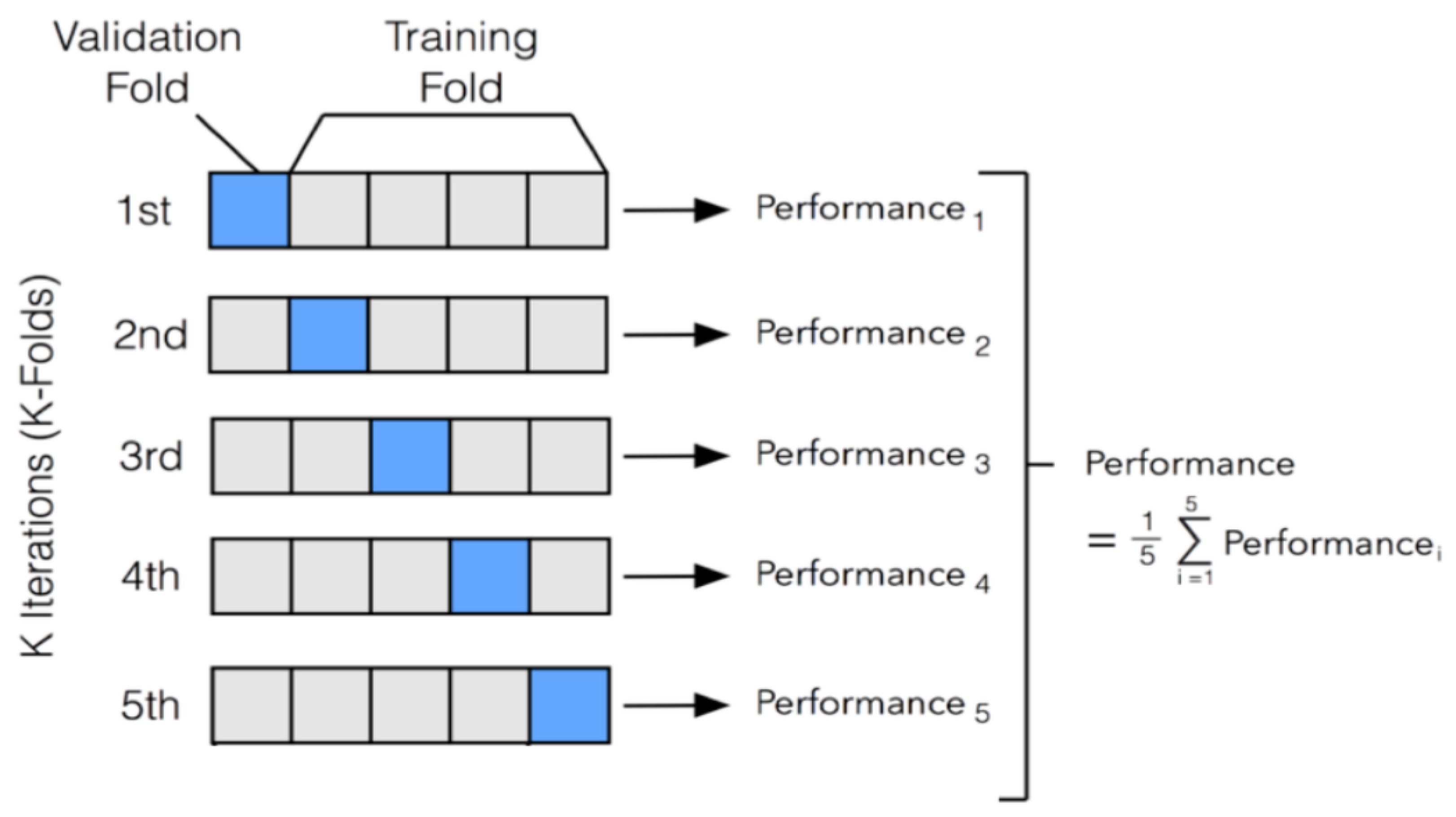
We performed 5-fold stratified cross-validation to evaluate model performance on training data. Figure 2 illustrates the stratified 5-fold cross-validation approach used.

From Figure 2, the dataset was partitioned into five mutually exclusive and approximately equal-sized subsets called folds. During each iteration, four folds were used for model training while the remaining fold served as the validation set. This process was repeated five times, with each fold serving once as the validation set and four times as part of the training set. Performance metrics based on F1 score were computed independently for each iteration, and the overall performance of the model was obtained by averaging the metrics across all five folds.

Six different machine learning models were evaluated: logistic regression (LR), support vector machine (SVM), three decision tree ensemble methods (random forest (RF), gradient boosting machine (GBM), and extreme gradient boosting (XGB)), and an artificial neural network (ANN) model. The models were tuned with different hyperparameter settings based on several iterations of empirical testing and recommendations from prior research. The tuning process was guided by iterative experimentation and established recommendations from prior research. While we did not employ an automated grid or random search approach, hyperparameters were adjusted through multiple empirical runs using 5-fold stratified cross-validation to balance overfitting and underfitting.

Table 3. Hyperparameter adjustments used for machine learning algorithm optimization.

Model	Hyper Parameters
LR	max_iter = 500
SVM	max_iter = 500, kernel = rbf
RF	n_estimators = 100, max_depth = 10, min_samples_split = 5
GBM	n_estimators = 50, max_depth = 5, min_samples_split = 5
XGB	n_estimators = 50, max_depth = 5, min_samples_split = 5
ANN	optimizer = Adam, learning_rate = 0.0005

presents the final hyperparameter adjustments made to each model type.

The LR model was trained with a maximum iteration threshold of 500 (max_iter = 500) to permit sufficient transformation space for convergence, given the possibility of slow convergence in high-dimensional data. The maximum iteration of the SVM was also set to 500, with a radial basis function (RBF) kernel, which is well suited for capturing non-linear decision boundaries. The RF model was configured with 100 decision trees (n_estimators = 100). A maximum tree depth of 10 (max_depth = 10) was set to control overfitting. Additionally, a minimum requirement of five samples was allowed to split an internal node (min_samples_split = 5), which promoted generalization by restricting overly specific splits. The GBM model was set to perform 50 boosting iterations (n_estimators = 50) with each base learner constrained to a maximum tree depth of 5 (max_depth = 5). Similar to the RF model, a minimum sample split of 5 was set. The XGB hyperparameters were adjusted similarly to the GBM (n_estimators = 50, max_depth = 5, min_samples_split = 5). The XGB algorithm further leverages regularization and parallel processing to optimize performance and computational efficiency. A multilayer perceptron (MLP) was used, and the ANN algorithm was designed with three hidden layers. The architecture comprised a primary dense layer with 64 units followed by a dropout rate of 0.2, a second dense layer with 32 units and dropout rate of 0.2, and a third dense layer with 16 units followed by dropout of 0.1. The dropout layers were incorporated to mitigate overfitting by randomly deactivating a proportion of neurons during training. The model was compiled using the Adam optimizer with a 0.0005 learning rate.

The confusion matrix was mainly used to evaluate algorithm performance [39]. This matrix provided the metrics on non-defaulters accurately classified (true positives (TPs)), defaulters accurately classified (true negatives (TNs)), defaulters classified as non-defaulters (false positives (FPs)), and non-defaulters classified as defaulters (false negatives (FNs)). Measurements of accuracy, precision, recall/sensitivity, and F1 score were computed as key performance indicators. The Receiver Operating Characteristic (ROC) curve and the Area Under the Curve (AUC) were also computed, with the distance of the ROC curve above the diagonal random classifier line (AUC = 0.5) used to determine how significantly the algorithms performed against random guessing.

Lastly, significance testing of models was performed using the DeLong test function [40] to compare the areas under two or more ROC curves and to determine whether the difference in AUC between two models was statistically significant.

3. Results

A total of 13,724 records comprising 158 features were extracted from two independent survey rounds. Among these, 51 features held data on household asset ownership, serving as proxies for PCA wealth index estimation. Also, 28 features held data on the administration of various vaccines and their dates of administration. Of the total records analysed, 69.54% (n = 9544) were classified as defaulters, whereas 30.46% (n = 4180) were categorized as non-defaulters. The class distribution of defaulters and non-defaulters is presented in

Table 4. Class distribution of defaulters and non-defaulters.

Class Distribution	Total (%)	Percentage
Defaulters	9544	69.54
Non-defaulters	4180	30.46
Total	13,724	100.00

.

It is worth noting here that a significantly larger proportion of defaulters came from the baseline survey (62.52%), while the majority of non-defaulters emanated from the end-point survey (84.09%). Both surveys employed identical instruments with no major changes in vaccine policy.

3.1. Results on SMOTE and Data Augmentation

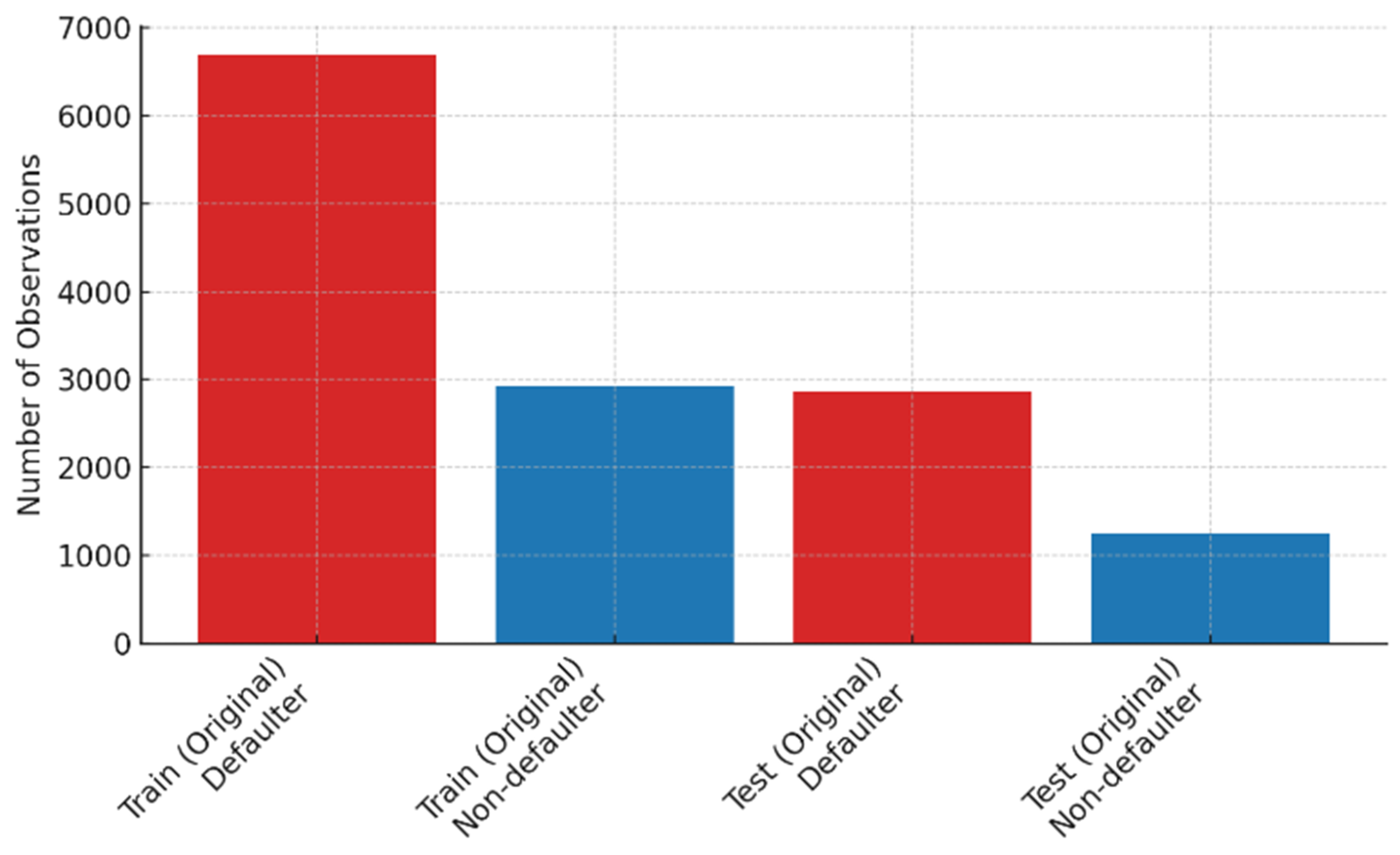
After train–test splitting, 69.6% (n = 6680) of the training data represented the defaulter class, while 2926 (30.4%) records belonged to the non-defaulter class. Similarly, in the test set, the defaulter class constituted 2864 (69.5%) records, while 1254 (30.5%) belonged to the non-defaulter class. These distributions indicated class imbalance in both training and test subsets. Figure 3 shows the imbalance in defaulter and non-defaulter classes within the original training and test sets, with approximately 70% of records representing the defaulter class.

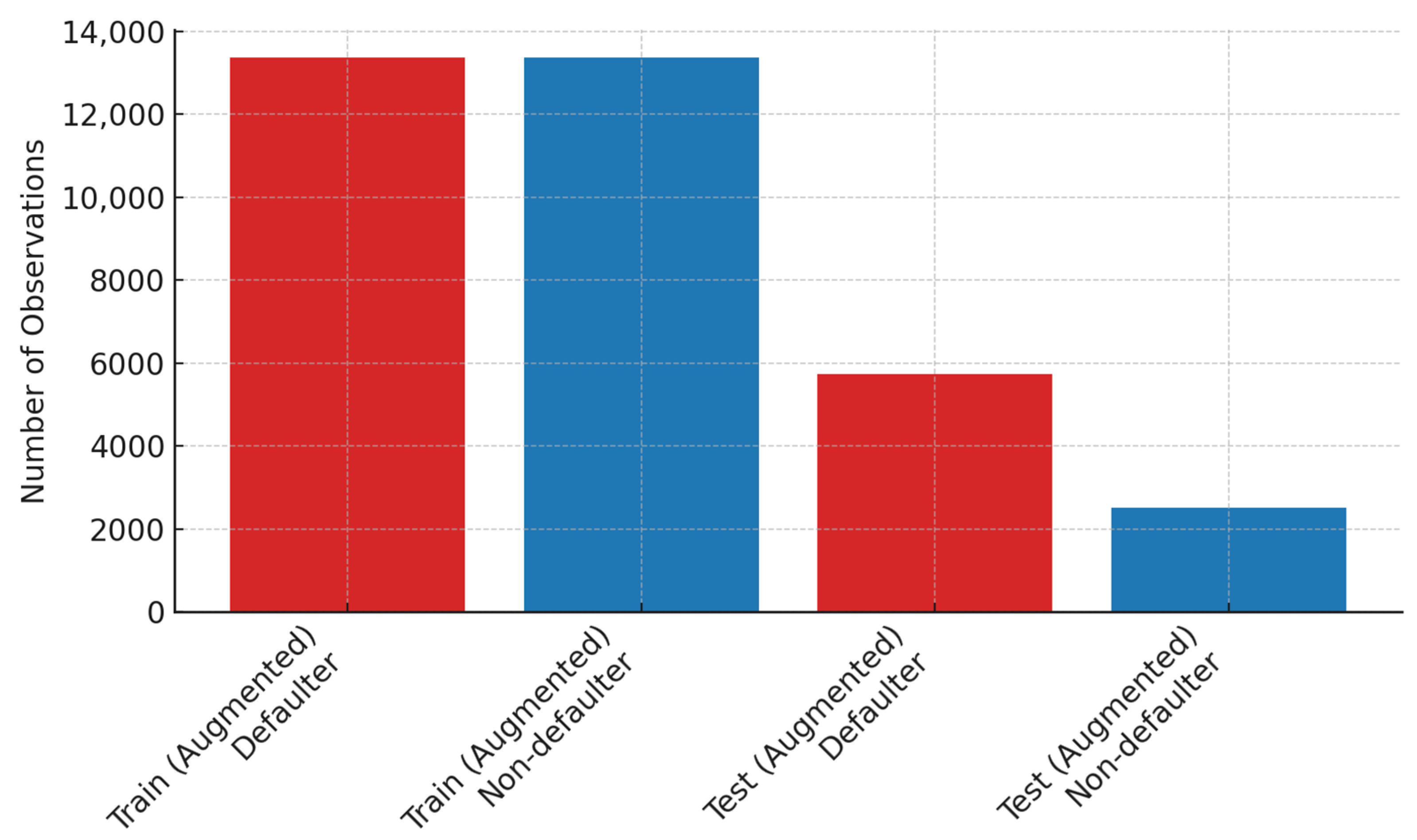
The bar graphs in Figure 4 show the results of the balanced class distribution achieved after DA and using the SMOTE.

Figure 4 shows that the techniques applied resulted in an expanded training set of 26,744 observations with a perfectly balanced distribution of non-defaulters (n = 13,372) and defaulters (n = 13,372). DA on the test dataset expanded the original records to 8235 observations, with 5731 (69.6%) for the defaulter class and 2504 (30.4%) belonging to the non-defaulter class.

3.2. Exploratory Data Analysis

In this section, we provide a descriptive analysis of the features used for predicting childhood vaccination defaulter risk. The descriptive analysis is based on the total number of records (n = 13,724) obtained. The results are a cross-analysis of features and their distribution between the defaulter and non-defaulter classes. For all categorial features, the results include the p-value computed using the chi-square test for statistical significance testing.

3.2.1. Demographic Characteristics

The demographic characteristics of each child covered sex and age distributions. Sex distribution by defaulter and non-defaulter classes is presented in

Table 5. Sex distribution of defaulters and non-defaulters.

Child’s Sex	DEFAULTERS (n = 9544)		NON-DEFAULTERS (n = 4180)		p-Value
	n	%	n	%
Female	4705	49.30	2017	48.25	0.260
Male	4839	50.70	2163	51.75

.

We can see from the results that the association between sex and defaulting from childhood immunization was not statistically significant. There was approximately a 50% split between females and males for both the defaulter and non-defaulter classes. Following this, a statistical summary of age distribution between defaulter and non-defaulter children is presented in

Table 6. Sex distribution of defaulters and non-defaulters.

Distribution by Age	DEFAULTERS (n = 9544)	NON-DEFAULTERS (n = 4180)
Minimum	5	5
Maximum	48	48
Mean	26.50	23.35
Standard Deviation	12.85	12.92
25th Percentile (Q1)	15.75	10.00
Median (Q2)	26.50	24.00
75th Percentile (Q3)	37.25	34.00

.

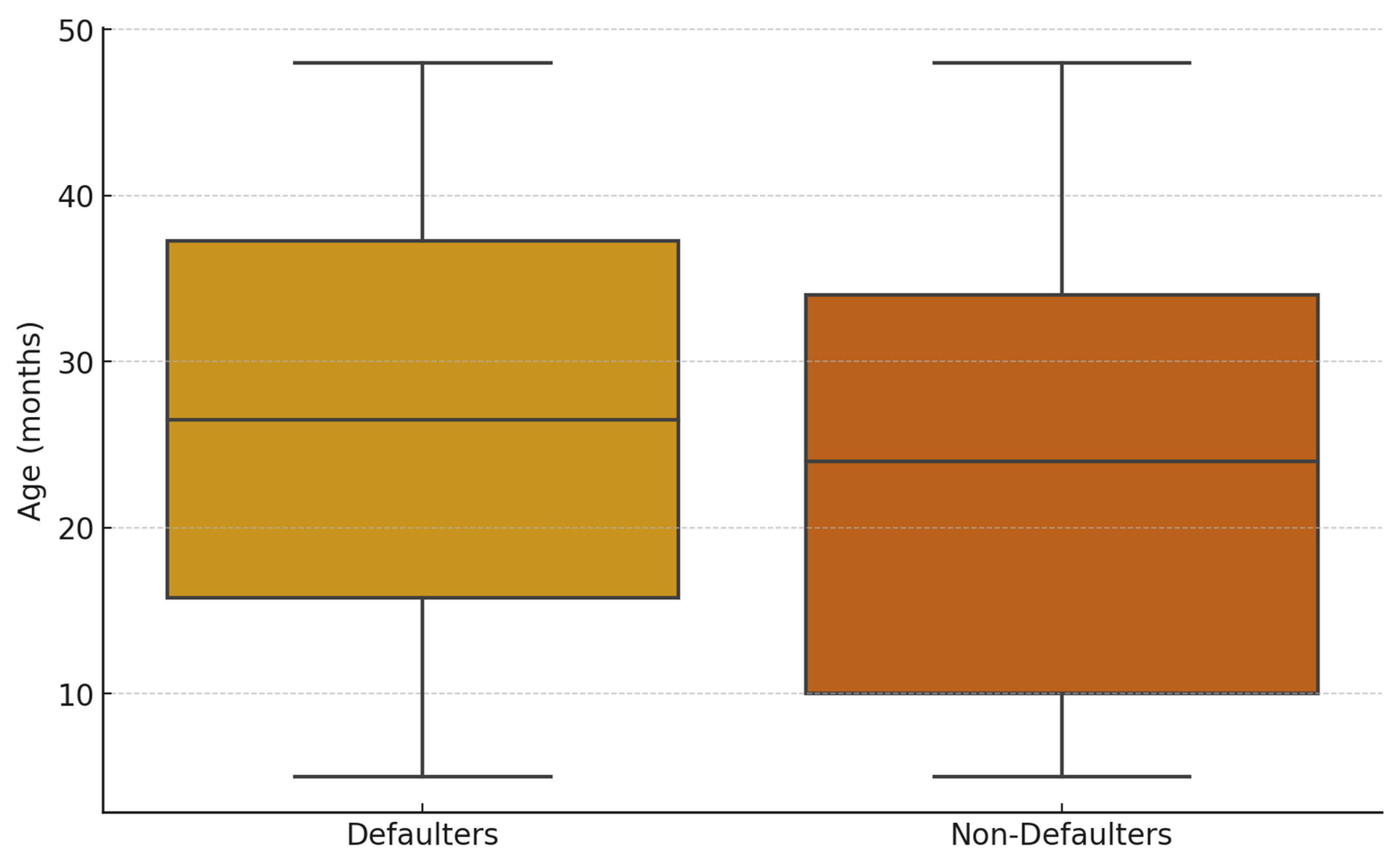
The age distribution of children, on the other hand, differed between the two classes (Figure 3). The non-defaulter class had a lower mean age (23.4, ±12.92) compared to the defaulter class (26.5, ±12.85). Both classes had the same minimum (5 months) and maximum (48 months) ages. However, the age distribution was skewed towards older children for the defaulter class (Figure 5).

In addition to the child’s socio-demographics, the analysis included the socio-demographics of the caregiver (education, employment, etc.) as well as health practices related to childcare such as bed net use and health insurance coverage. A tabular summary of the analysis of caregiver socio-demographics is presented in Table A1 in Appendix A. From the results, we observed higher educational attainment among the non-defaulter class. For instance, a higher number of non-defaulters had attained senior secondary level (16.56%), compared to defaulters (11.67%), and tertiary education (5.33%), compared to defaulters (3.15%). Maternal employment status between the two classes was comparable, with self-employment being the most common occupation, forming approximately 40% in both classes. In terms of child healthcare practices, 54.11% of non-defaulters had health insurance coverage, compared to 48.58% for defaulters. Similarly, mosquito net usage was higher among non-defaulters (67.27%) compared to defaulters (64.13%). Predictors categorised under household characteristics include socio-economic status, household composition, settlement type (rural/urban), and the hygienic status of essential utilities (toilet facilities and source of water). There were also differences in socio-economic status between defaulters and non-defaulters. A higher proportion of non-defaulters were classified as wealthy (23.30%) compared to defaulters (18.51%), while a smaller proportion of non-defaulters fell into the “poor” and “low” categories (16.39% and 19.02%, respectively) compared to defaulters (21.80% and 21.13%). In subjective assessments of wealth status, a similar pattern was observed. Over half of the non-defaulter class (51.10%) perceived themselves as being in the “average” or better wealth categories, compared to 45% of defaulters. Fewer individuals under the non-defaulter class considered themselves “poor” (9%) compared to defaulters (13.47%). The results on household composition present the relationship of the household head to the child. Slightly more non-defaulters had the child’s father as the head of household (53.97%) compared to defaulters (52.88%). With respect to settlement type, a marginally higher proportion of the non-defaulter class resided in rural settlements (58.21%) compared to defaulters (56.83%). Concerning the analysis of hygienic status predictors, access to a hygienic toilet facility was reported by 45.43% of non-defaulters, compared to 40.38% of defaulters. Similarly, clean energy use for cooking was more common among non-defaulters (14.09%) than defaulters (10.12%). Both groups, however, reported high access to a hygienic source of water, though this was slightly higher among non-defaulters (89.16%) than among defaulters (86.53%). In terms of statistical significance, the associations between all of the maternal characteristics analysed and childhood vaccination defaulting had a p-value < 0.001.

3.2.2. Timing of Vaccination and Birth

In this section, descriptive summaries on vaccination timing and season of birth are presented.

Table 7. Analysis of on-time vaccination by defaulters and non-defaulters.

Ontime Vaccination	DEFAULTERS (N = 9544)		NON-DEFAULTERS (N = 4180)		p-Value
	n	%	n	%
At birth	5989	62.75	3533	84.52	<0.001
At week—6	5377	56.34	2873	68.73	<0.001
At week—10	4073	42.68	2350	56.22	<0.001
At week—14	3054	32.00	1830	43.78	<0.001
At month—6	203	2.13	86	2.06	0.794
At month—9	239	2.50	77	1.84	0.017
At month—12	15	0.16	7	0.17	0.890
At month—18	29	0.30	10	0.24	0.513

presents the distribution of children who received vaccination within the on-time window for age.

From the results, a decreasing trend in on-time vaccination is observed for both classes. At birth, 62.75.3% of children within the defaulter class received their vaccine dose on time, compared to 84.52% of non-defaulters. At 6 weeks, 56.34% of defaulters received the dose on time versus 68.73% of non-defaulters. This decreased further at 10 weeks (42.68% vs. 56.22%) and at 14 weeks, where 32% of children within the defaulter class received the dose on time, compared to 43.78% of those in the non-defaulter group. Timely vaccination at the later schedule dates was extremely low, with inconsistent distributions between the defaulter and non-defaulter classes. We further examined off-time vaccination windows by early and delayed vaccination.

Table 8. Analysis of early vaccination by defaulters and non-defaulters.

Early Vaccination	DEFAULTERS (N = 9544)		NON-DEFAULTERS (N = 4180)		p-Value
	n	%	n	%
At week—6	109	1.14	60	1.44	0.152
At week—10	113	1.18	45	1.08	0.587
At week—14	119	1.25	49	1.17	0.715
At month—6	97	1.02	28	0.67	0.049
At month—9	251	2.63	86	2.06	0.046
At month—12	98	1.03	131	3.13	<0.001
At month—18	325	3.41	187	4.47	0.002

presents the results of vaccinations administered earlier than the expected window.

Overall, early vaccination was an infrequent event across both classes, with proportions generally below 5% at all timepoints. At week 6, 1.14% of defaulters and 1.44% of non-defaulters received vaccines early (p = 0.152). Similar marginal differences were observed at week 10 (1.18% vs. 1.08%) and week 14 (1.25% vs. 1.17%). These findings suggest no significant difference in early vaccination uptake between the groups during the foundational stages of the immunization schedule. At month 6, however, a higher proportion of defaulters (1.02%) received early vaccines compared to non-defaulters (0.67%). The difference widened at month 9, with 2.63% of defaulters vaccinated early compared to 2.06% of non-defaulters. A reversed trend was observed for the last two schedule dates. At month 12, non-defaulters were significantly more likely to receive vaccines early (3.13%) compared to defaulters (1.03%). At month 18, a proportion of 4.47% of the non-defaulter class received early vaccination compared to 3.41% of the defaulter class. The results on delayed vaccination show significant differences in distributions, with a higher number from the defaulter class reporting delays in the first four schedules. The results for delayed vaccination are presented in

Table 9. Analysis of delayed vaccination by defaulters and non-defaulters.

Delayed Vaccination	DEFAULTERS (n = 9544)		NON-DEFAULTERS (n = 4180)		p-Value
	n	%	n	%
At birth	2893	29.75	583	13.95	<0.001
At week—6	3864	40.49	1227	29.35	<0.001
At week—10	5105	53.49	1757	42.03	<0.001
At week—14	5936	62.20	2281	54.57	<0.001
At month—6	7473	78.30	3627	86.77	<0.001
At month—9	7323	76.73	3116	74.55	0.006
At month—12	3156	33.07	2538	60.72	<0.001
At month—18	4179	43.79	2479	59.31	<0.001

.

At birth, 29.75% of defaulters reported delayed vaccination compared to 13.95% of non-defaulters (p < 0.001). At week 6, 40.49% of defaulters reported delayed vaccination compared to 29.35% of non-defaulters (p < 0.001). Similar trends, with statistically significant differences (p < 0.001), were observed at week 10 (53.49% of defaulters versus 42.03% of non-defaulters) and at week 14 (62.20% of defaulters versus 54.57% of non-defaulters). At month 6, however, a higher proportion of non-defaulters (86.77%) reported delayed vaccination compared to defaulters (78.30%), with a statistically significant difference observed (p < 0.001). At month 9, the difference was marginal, with 76.73% of defaulters and 74.55% of non-defaulters reporting delays (p = 0.006). Again, a reverse trend was observed at months 12 and 18. 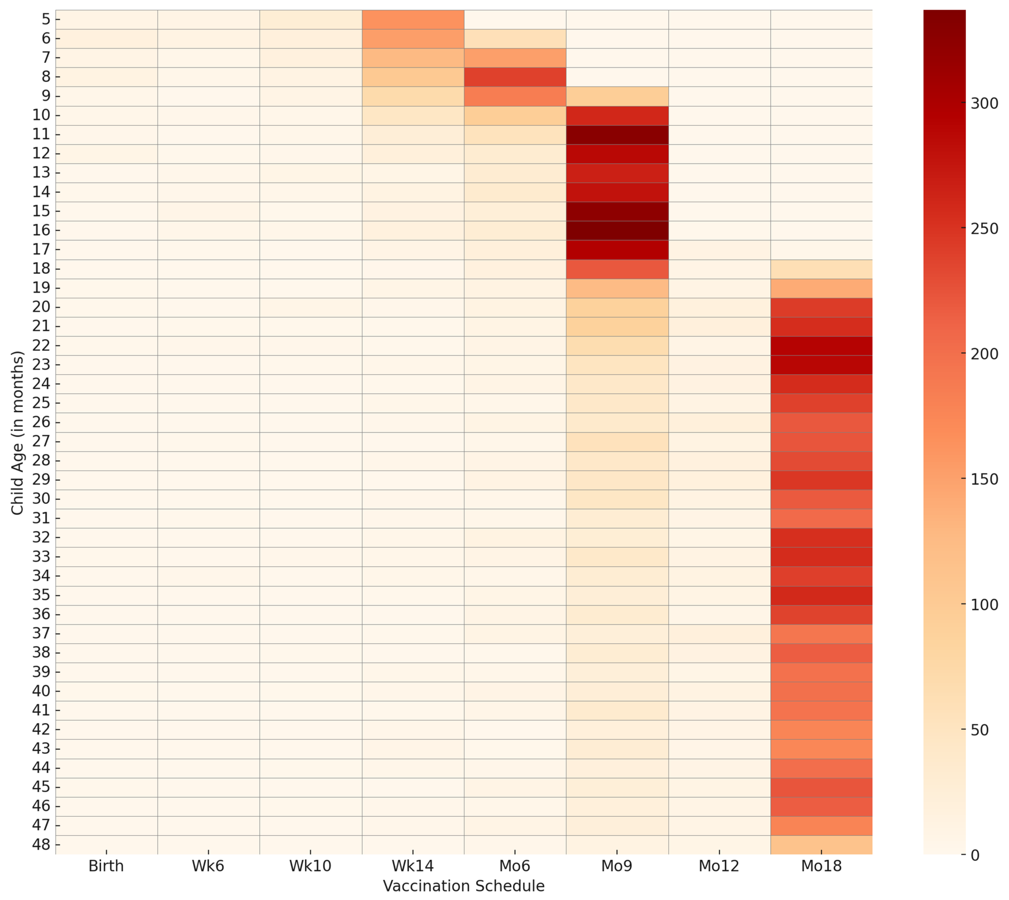A significant proportion of non-defaulters reported delayed vaccinations at month 12, 60.72% compared to 33.07% of defaulters (p < 0.001), and at month 18, 59.31% compared to 43.79% of defaulters (p < 0.001). A heatmap for visualising delayed vaccination by age and vaccination timing is presented in Figure 6.

From Figure 6, we can observed that delayed vaccination is marginal in frequency. The map shows an increased frequency of delayed vaccination, particularly for months 9 and 18. The results on birth seasonality (

Table 10. Analysis of birth season by defaulters and non-defaulters.

Birth Season	DEFAULTERS (n = 9544)		NON-DEFAULTERS (n = 4180)		p-Value
	n	%	n	%
Major rainy season	3553	37.23	1801	43.09	<0.001
Minor rainy season	1634	17.12	670	16.03
Dry season	3569	37.40	1351	32.32

) reveal statistically significant associations (p < 0.001) between season of birth and vaccination default.

From the results presented in Table 10, we can see that children born during the major rainy season constituted the largest proportion of non-defaulters (43.09%) compared to 37.23% of defaulters. For the minor rainy season, the distribution was relatively similar across groups, with 17.12% of defaulters and 16.03% of non-defaulters born during this period. Conversely, children born in the dry season were more likely to be defaulters (37.40%) than non-defaulters (32.32%).

3.3. Cross-Validation of Training Data

This section presents results on model training validation using both the original and augmented data.

Table 11. Average F1 score for 5-fold cross-validation on original and augmented datasets.

Model	Average F1 Score
	Weighted (Original)	Macro (Original)
LR	0.8284 (±0.0037)	0.7940 (±0.0037)
SVM	0.6950 (±0.0351)	0.6646 (±0.0348)
RF	0.8565 (±0.0067)	0.8254 (±0.0085)
GBM	0.8731 (±0.0080)	0.8491 (±0.0090)
XGB	0.8747 (±0.0052)	0.8515 (±0.0058)
ANN	0.8440 (±0.0041)	0.8136 (±0.0049)

presents the mean scores from the 5-fold stratified cross-validation performed on both datasets. For each model, the average macro and weighted F1 scores are presented for the original imbalanced data, while only the macro average is presented for the balanced data. Corresponding standard deviations are also reported to provide information on performance variability and model stability.

The results generated from the original data show that the GBM model reported the highest average F1 scores of 0.8730 (±0.0044) for weighted and 0.8489 (±0.0051) for macro. The mean scores of the XGB and RF models were marginally lower. The XGB model reported a weighted F1 score of 0.8687 (±0.0063) and a macro F1 score of 0.8445 (±0.0070), while the RF model reported 0.8592 (±0.0081) for weighted F1 score and 0.8299 (±0.0098) for macro F1 score. The ANN model, on the original data, reported relatively high average weighted (0.8440 (±0.0041)) and macro (0.8136 (±0.0049)) F1 scores. The results from the 5-fold cross-validation are presented in boxplots in Figure 7.

The ANN model results were lower than those reported by the three ensemble methods but higher than those reported by the LR and SVM models. The average F1 scores reported by the SVM were below 80%, with a weighted F1 score of 0.6950 (±0.0351) and a macro F1 score of 0.6646 (±0.0348). Overall, ensemble tree classifiers (GBM, XGB, RF) yielded better classification performance compared to the other models during cross-validation on the original data.

The results from the augmented data (

Table 12. Average F1 score for 5-fold cross-validation on original and augmented datasets.

Model	Average F1 Score
	Macro (Augmented)
LR	0.8458 ± 0.0039
SVM	0.7516 ± 0.0445
RF	0.8881 ± 0.0060
GBM	0.8805 ± 0.0121
XGB	0.9035 ± 0.0230
ANN	0.9043 ± 0.0057

) showed comparatively improved F1 scores across all models.

The SVM reported an increase in macro F1 score from 0.6646 ± 0.0348 to 0.7516 ± 0.0445. Similarly, the ANN and XGB models showed improvements in F1 score post augmentation, with the ANN’s score increasing from 0.8136 ± 0.0049 to 0.9043 ± 0.0057 and XGB’s score increasing from 0.8515 ± 0.0058 to 0.9035 ± 0.0230. The scores of high-performing RF and GBM models also increased with data augmentation. The RF model’s macro F1 score increased from 0.8254 ± 0.0085 to 0.8881 ± 0.0060, while the GBM model’s score rose from 0.8491 ± 0.0090 to 0.8805 ± 0.0121. Thus, after augmentation, the RF model reported the highest performance. Cross-validation results from the augmented data are presented as boxplots in Figure 8.

3.4. Model Training Behaviour Analysis

In this section, we present the results on the learning behaviour of the models during training. We show the observed F1 score distributions from different training and validation data sizes both before and after data augmentation. For the first five models, we present learning behaviour curves based on the mean F1 scores with standard deviations. For the ANN model, we present learning curves from validation loss metrics at different epochs. Visualizations of the learning curves are presented in Appendix B.

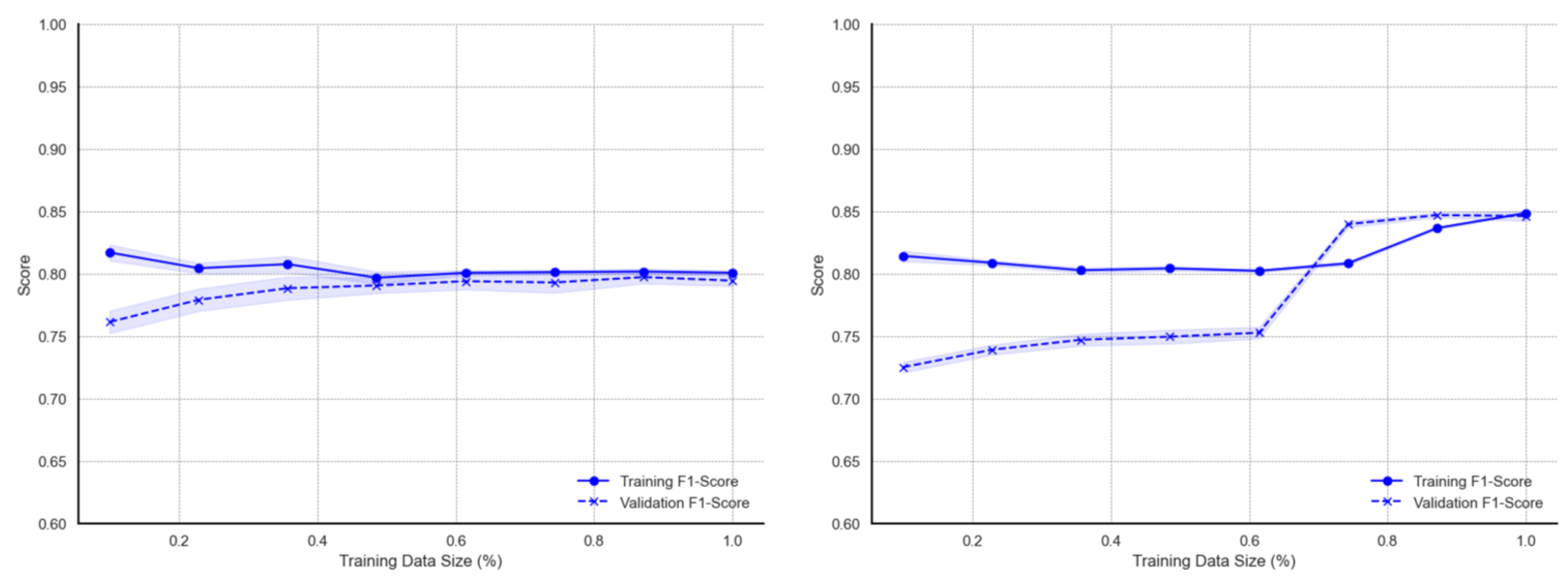
As seen in Figure A1, the learning curves of the LR on the original data exhibit minimal deviations throughout the different data sizes. The curves show decreasing deviations from average F1 scores and convergence over larger data sizes. On the augmented dataset, LR training and validation F1 curves converge at a 100% data size. However, there are observable deviation measurements of validation F1 scores for data sizes below 60%. Generally, LR learning curves show more noticeable performance improvement on the augmented dataset compared to the original dataset. For the SVM model, however, the learning curves (Figure A2) show different patterns of behaviour between the original and augmented dataset. The training F1 scores are higher for smaller data sizes between 20% and 40%, after which the F1 scores continuously decrease over larger datasets. The persistent decrease in performance is coupled with increased deviations from the mean. Model learning improvement for the SVM model on the augmented data is mainly seen in reduced deviations from the mean F1 score as well as narrowed gaps between training and validation accuracy. Interestingly, the learning curves from the augmented dataset exhibit a study decline in F1 scores as the proportion of training data increases from 40% to approximately 76%, after which the F1 scores begin to increase.

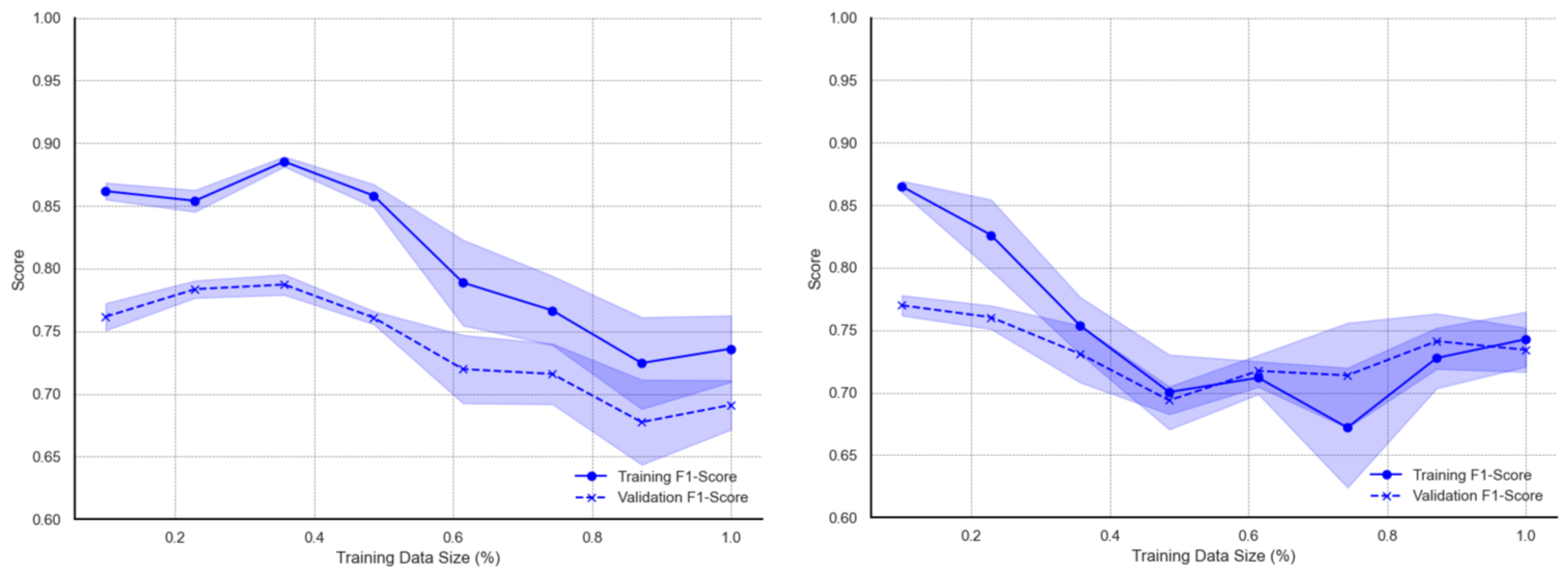
Curves for the ensemble models show more marginal deviations and better learning behaviour. The curves for the RF model (Figure A3) on the original data report approximately 0.98 when trained on smaller data subsets. As the training data size increases, the F1 score gradually declines possibly due to the increased variability and noise introduced with more data. Nonetheless, training scores remain above 0.88. On the other hand, the metric associated with validation data increases with more training data, with F1 score improving from ~0.76 to ~0.84. The initial performance gap between training and validation scores is largest at small training sizes, indicating possible overfitting over smaller data sizes. Marginal deviations are visible on the validation F1 curve. With regards to augmented data, learning curves of the RF model indicate relatively high (approximately 0.93–0.95) training F1 measurements for data sizes below 20%. There are similar declines up to a ~60–70% training size but then slightly increases towards the full data size. Validation curves, on the other hand, show a consistent upward trend across all training data sizes. F1 scores increases consistently from about 0.78 to approximately 0.89–0.91 at the full data size. Also, deviations from the average F1 score are smaller compared to those observed using the original data. 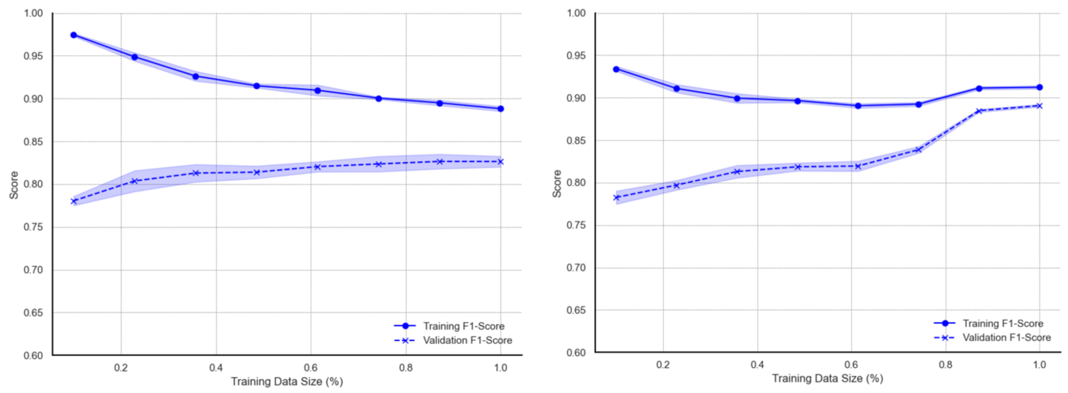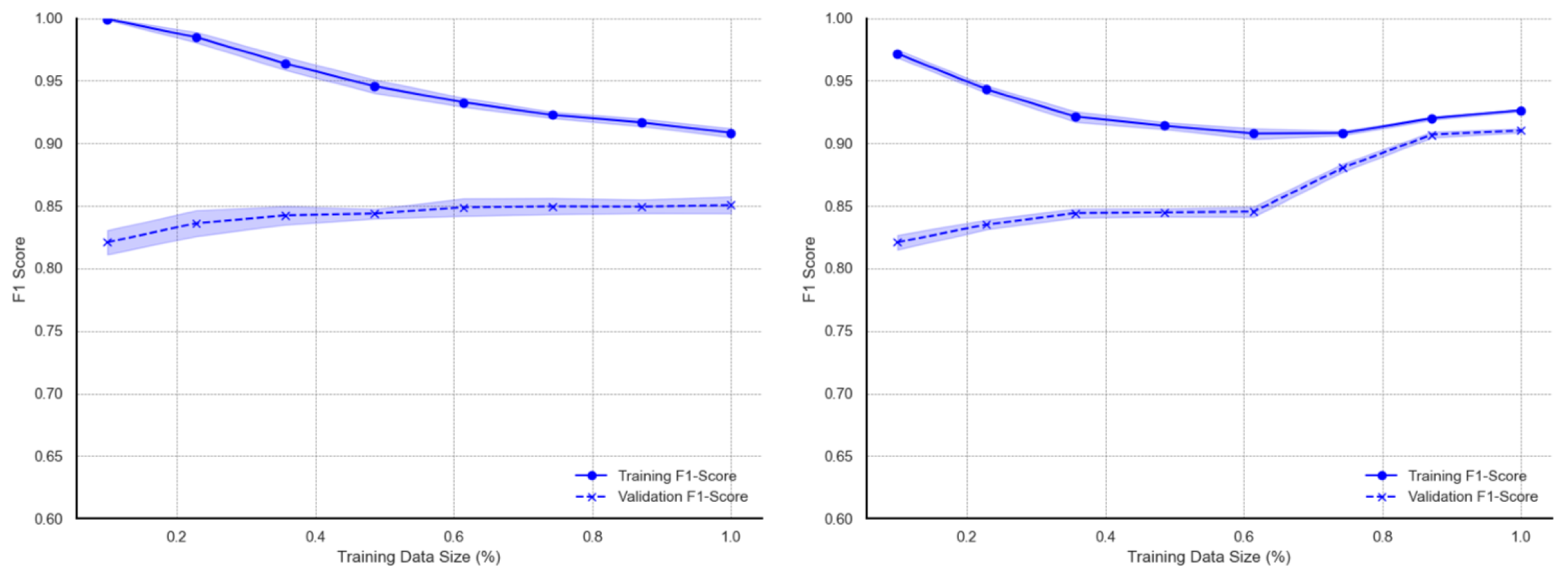As with the RF ensemble classifier, learning curves for the GBM model (Figure A4) report high F1 scores for smaller training subsets and continuous decline with larger subsets. Metric scores on validation data exhibit a gradual increase with observable deviations from the mean. When trained with the augmented data subsets, the decreasing trend of training learning curves over larger subsets is observed up to around 70% of training data, after which the metric scores tend to marginally rise toward the full dataset size. The validation learning curves for augmented data show steady growth with increasing data sizes. A more significant increase is observed within the 75–85% training data usage region, after which curves for both training and validation converge towards scores of 0.89 to 0.90 at full data use. The XBG model exhibits learning behaviours (Figure A5) similar to those of the GBM model. The training metrics for the XGB model show exceptionally high scores of almost 1.00 at the smallest training size before gradually decreasing to approximately 0.90 at the full data size. Validation metrics also show similar patterns to the GBM. On augmented data, the learning curves for XGB decreases and rises at a much larger training subset (80%) towards the full data size. As with the GBM model, the validation curves sharply increase, after which both training and validation curve metrics converge. This distinct increase in the validation F1 score for XGB, however, occurs earlier, starting at approximately 60% subset usage.

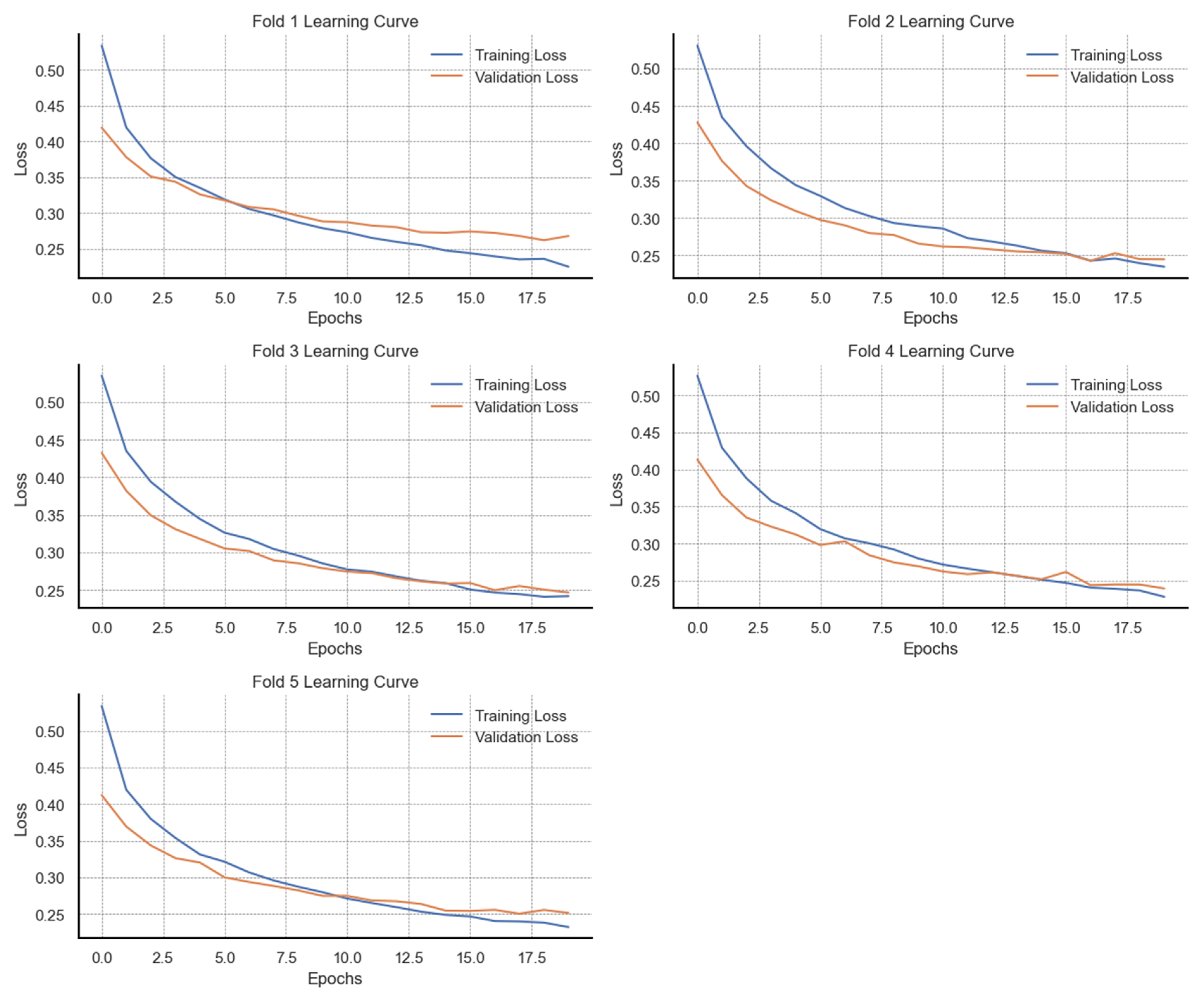
Figure A6 presents the learning behaviour of the ANN model through training and validation loss trajectories over 20 epochs across five cross-validation folds on the original data. With the original dataset, the results across all five folds demonstrate stable learning by a consistent reduction in training loss over all epochs. By the final epoch, training loss in each fold falls below 0.35, suggesting a strong fit to the training data. Validation loss also decreases in parallel with training loss during the initial epoch, reflecting good early generalization. However, beyond approximately 10 epochs, the validation loss curves in folds 1, 3, and 5 begin to either plateau or show marginal increases. In effect, a widening gap between training and validation loss is observed. This divergence suggests the onset of overfitting, where continued training improves performance on the training data at the expense of generalization. In contrast, folds 2 and 4 exhibit better alignment between training and validation loss, with both curves converging towards a common minimum by the final epoch. Patterns for comparison are illustrated in Figure A7, which presents the training and validation loss trajectories of the ANN model trained on synthetically balanced and augmented data. Across all five folds, training loss consistently decreases over the 20 training epochs with minimal fluctuations, indicating stable convergence. The final training loss values in each fold fall below 0.25, reflecting effective learning. Similarly, validation loss declines in parallel with training loss across all folds, with final values ranging between 0.25 and 0.28, closely matching the training loss. Unlike the patterns observed in the original dataset (Figure A6), there is no significant divergence between training and validation loss in the later epochs, suggesting improved generalization and a notable reduction in overfitting.

3.5. Performance Evaluation on Test Data

A comparative evaluation of model performance on test data from both the original imbalanced dataset and the augmented dataset was performed. The results on precision, recall, and F1 scores are presented in

Table 13. Performance results of machine learning models on unseen data.

Model	Class	Original Data			Augmented Data
		Precision	Recall	F1 Score	Precision	Recall	F1 Score
LR	Defaulters	0.86	0.90	0.88	0.87	0.86	0.87
	Non-defaulters	0.75	0.65	0.70	0.69	0.72	0.70
SVM	Defaulters	0.80	0.79	0.80	0.86	0.57	0.69
	Non-defaulters	0.54	0.55	0.54	0.45	0.80	0.57
RF	Defaulters	0.88	0.94	0.91	0.94	0.90	0.92
	Non-defaulters	0.84	0.70	0.77	0.79	0.87	0.83
GBM	Defaulters	0.90	0.93	0.91	0.93	0.89	0.91
	Non-defaulters	0.83	0.76	0.79	0.78	0.86	0.81
XGB	Defaulters	0.90	0.91	0.91	0.93	0.91	0.92
	Non-defaulters	0.80	0.77	0.79	0.81	0.85	0.83
ANN	Defaulters	0.87	0.92	0.89	0.91	0.93	0.92
	Non-defaulters	0.79	0.69	0.74	0.83	0.79	0.81

.

In identifying defaulters, LR reported a decrease in recall (from 0.90 to 0.86) after data augmentation, which subsequently decreased the F1 score (from 0.88 to 0.87). For non-defaulter classification, a significant increase in recall was reported (from 0.65 to 0.72) after data augmentation, resulting in a maintained F1 score of 0.70. The performance of the SVM model on the other hand showed inconsistencies. Despite an improvement in the precision in identifying defaulters, the F1 score declined (0.80 to 0.69) due to decreased recall from 0.79 to 0.57. However, the augmentation improved sensitivity to the minority non-defaulter class, where recall increased from 0.55 to 0.80, which improved the F1 score from 0.54 to 0.57. The ensemble classifier models reported improved F1 scores after data augmentation. The F1 score for the defaulter class improved from 0.91 to 0.92, while the F1 score of the non-defaulter class also increased significantly from 0.77 to 0.83. With respect to the GBM model, the F1 score for the defaulter class remained the same at 0.91 after augmentation, while an improvement in recall (0.76 to 0.86) for the non-defaulter class enhanced the F1 score from 0.79 to 0.81. The XGB model also maintained high predictive performance for both classes. Among defaulters, the F1 score improved from 0.91 to 0.92, while the F1 score among non-defaulters also increased from 0.79 to 0.83. The ANN model indicated the most consistent improvement driven by balanced increases in precision and recall. The F1 score increased from 0.89 to 0.92 for the defaulter class, while for non-defaulters, the F1 score increased from 0.74 to 0.81. 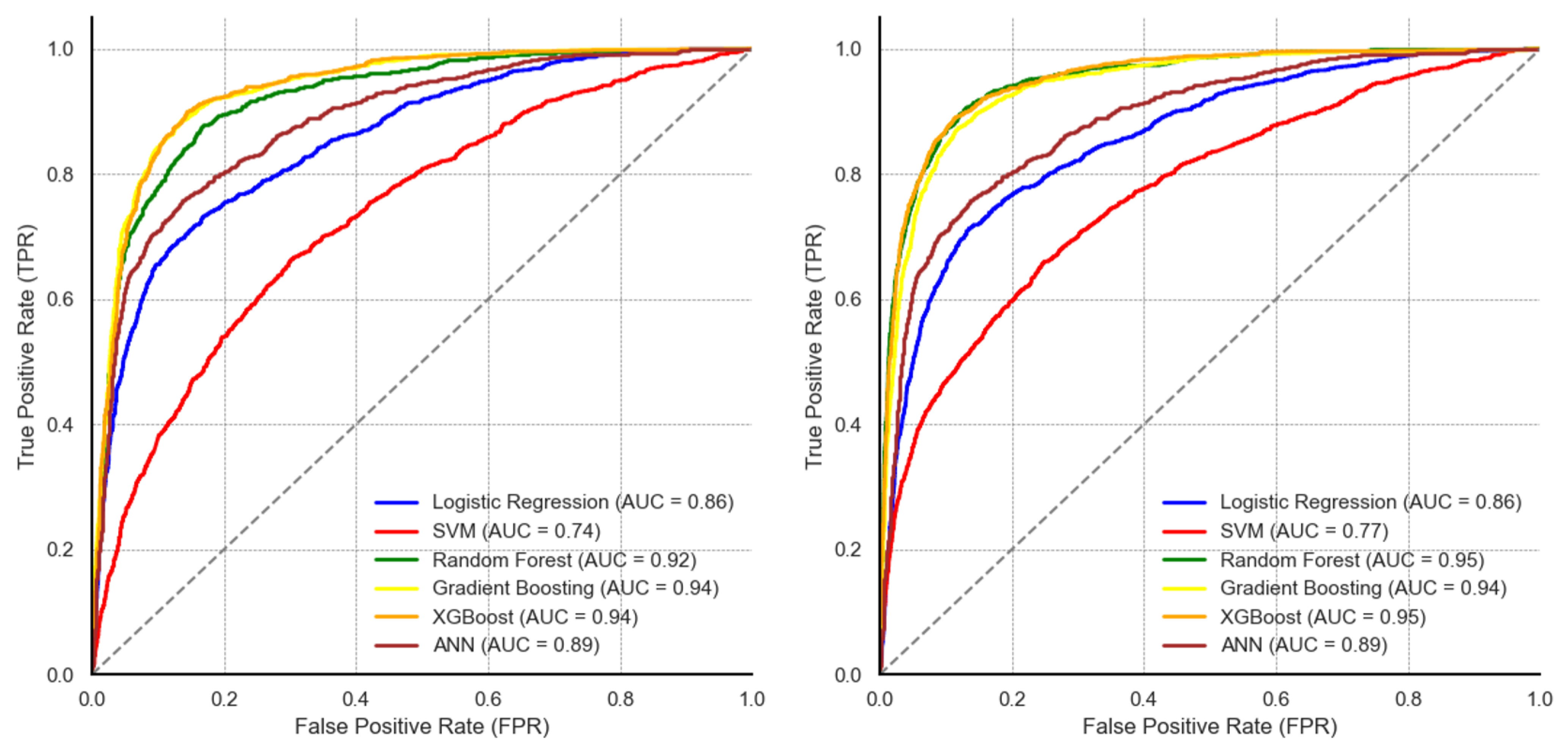Figure 9 illustrates the ROC curves and AUC values for the five machine learning models evaluated on unseen data.

On the original dataset, the ensemble-based classifiers reported comparative performance with an AUC of 0.92 for RF, 94 for the GBM, and 94 for XGB. The ANN reported an AUC of 0.88, while the SVM reported the lowest AUC of 0.74. Following data augmentation, there were observable differences in the AUC values. RF and XGB reported the highest AUC of 0.95 each, the AUC value of the ANN model increased from 0.88 to 0.93. On the other hand, LR and the GBM maintained the same AUC values compared to their performance on the original data. Although the SVM’s AUC increased from 0.74 to 0.77, the model still reported the lowest AUC.

The results from the DeLong significance test are presented in

Table 14. A table showing the significance test result for the models evaluated.

Model Comparison		Original Data				Augmented Data
		AUC1	AUC2	p-Value	z-Stat	AUC1	AUC2	p-Value	z-Stat
LR	SVM	0.86	0.74	<0.001	−14.50	0.86	0.77	<0.001	−14.56
LR	RF	0.86	0.92	<0.001	−14.42	0.86	0.95	<0.001	−25.76
LR	GBM	0.86	0.94	<0.001	−16.24	0.86	0.94	<0.001	−23.38
LR	XGB	0.86	0.94	<0.001	−15.75	0.86	0.95	<0.001	−25.07
LR	ANN	0.86	0.88	<0.001	−7.98	0.86	0.93	<0.001	−20.67
SVM	RF	0.74	0.92	<0.001	−22.71	0.77	0.95	<0.001	−32.44
SVM	GBM	0.74	0.94	<0.001	−24.77	0.77	0.94	<0.001	−31.22
SVM	XGB	0.74	0.94	<0.001	−24.73	0.77	0.95	<0.001	−32.93
SVM	ANN	0.74	0.88	<0.001	−18.58	0.77	0.93	<0.001	−28.87
RF	GBM	0.92	0.94	<0.001	−7.54	0.95	0.94	<0.001	−7.386
RF	XGB	0.92	0.94	<0.001	−6.10	0.95	0.95	0.342	−0.950
RF	ANN	0.92	0.88	<0.000	−10.72	0.95	0.93	<0.001	−9.799
GBM	XGB	0.94	0.94	0.451	−0.75	0.94	0.95	<0.001	−10.941
GBM	ANN	0.94	0.88	<0.001	−13.62	0.94	0.93	<0.001	−5.120
XGB	ANN	0.94	0.88	<0.001	−13.25	0.95	0.93	<0.001	−9.919

, using a threshold p-value < 0.05 to indicate a significant difference in performance.

On the original dataset, all pairwise comparisons between LR and other models reported statistically significant differences in AUC values (p < 0.001), while z-statistics reported relatively high magnitudes (e.g., z = −14.42 for LR vs. RF; z = −16.24 for LR vs. GBM). We note that the difference between LR and the ANN, although significant, reported a relatively low magnitude (z = −7.98). Nonetheless, the highest magnitudes in significance were observed on pairwise comparisons between the SVM and the ensemble decision tree classifiers (e.g., z = −24.77 for SVM vs. GBM; z = −22.71 for SVM vs. RF), with all differences being significant. Among the ensemble classifiers, differences between AUC values of RF and the GBM as well as between RF and XGB were statistically significant but with a low magnitude ((p < 0.001, z = −7.54) and (p < 0.001, z = −6.10), respectively). There was no significant difference observed between the GBM and XGB (p = 0.451, z= −0.75) in the original dataset. After data augmentation, comparisons between LR and all other models remained significant (p < 0.001), with increased z-statistics for the ensemble classifiers (e.g., z = −25.76 for LR vs. RF, z = −25.07 for LR vs. XGB). However, the difference in AUC values between the GBM and XGB was significant, while the value difference between RF and XGB was no longer significant (p = 0.342).

The RF and XGB models reported the highest AUC (0.995) compared to all other models, with significant differences recorded against the GBM (p < 0.001) and the ANN (p < 0.001) models.

3.6. Identification of Key Predictors

In this section, we compare key predictors of vaccine default identified from the three most effective models (RF, GBM and XGB). The ensemble learning classifiers, over several years, have been well known for their efficiency in classification problems due to their ability to handle complex, high-dimensional data and provide robust predictive performance [41]. These methods operate by combining multiple decision trees to improve prediction accuracy and reduce overfitting, with several tuneable hyperparameters including the number of trees, the maximum depth of each tree, the number of features to consider during splitting, the minimum number of samples required to split a node, and the minimum number of samples required at the leaf node [42]. In a classification task, the RF model builds trees independently and uses majority voting among all the trees for final prediction. The GBM model differs from the RF model by building trees sequentially rather than independently. XGB basically presents an enhanced implementation of the GBM that includes additional regularization and parallel processing.

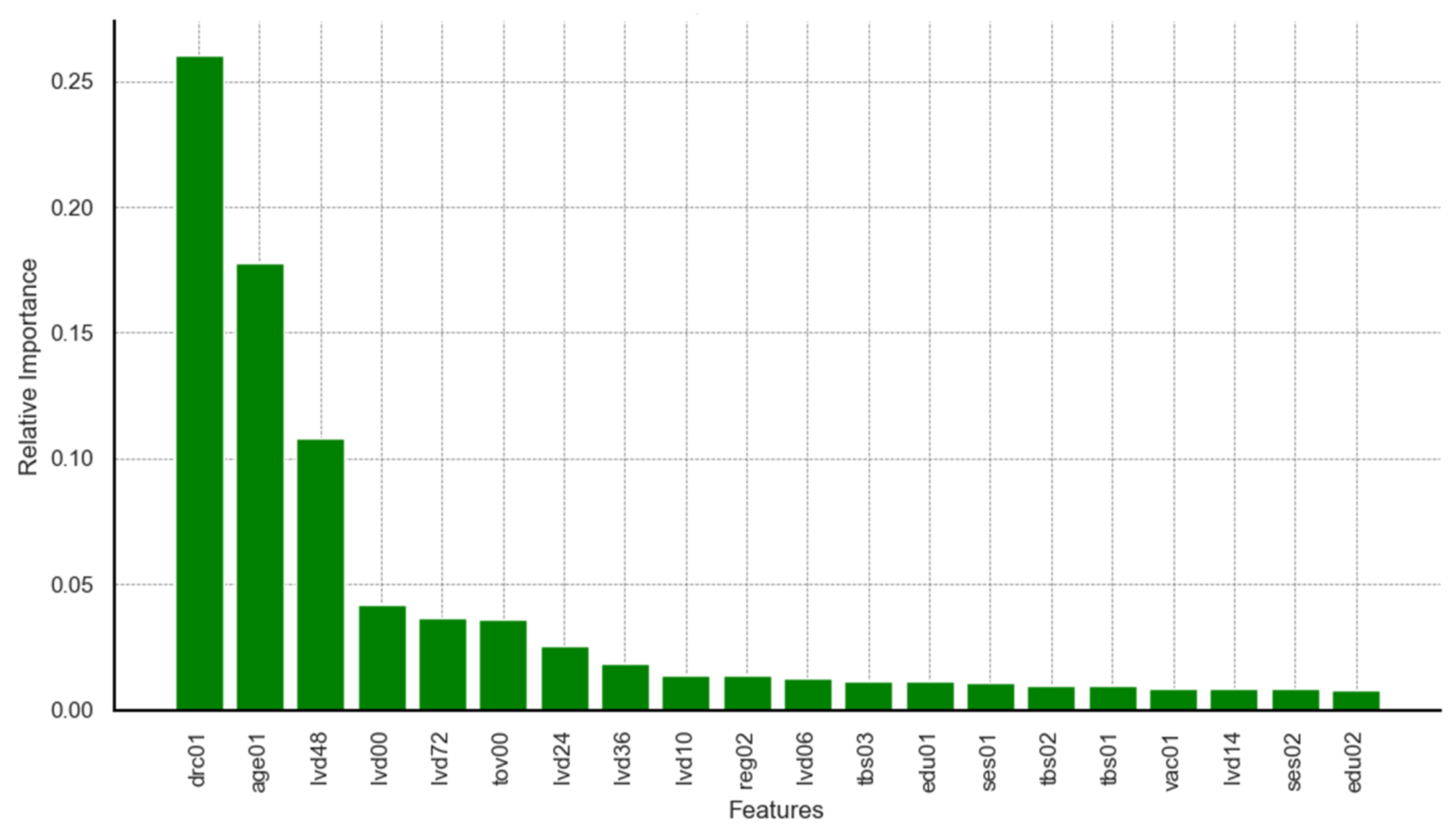
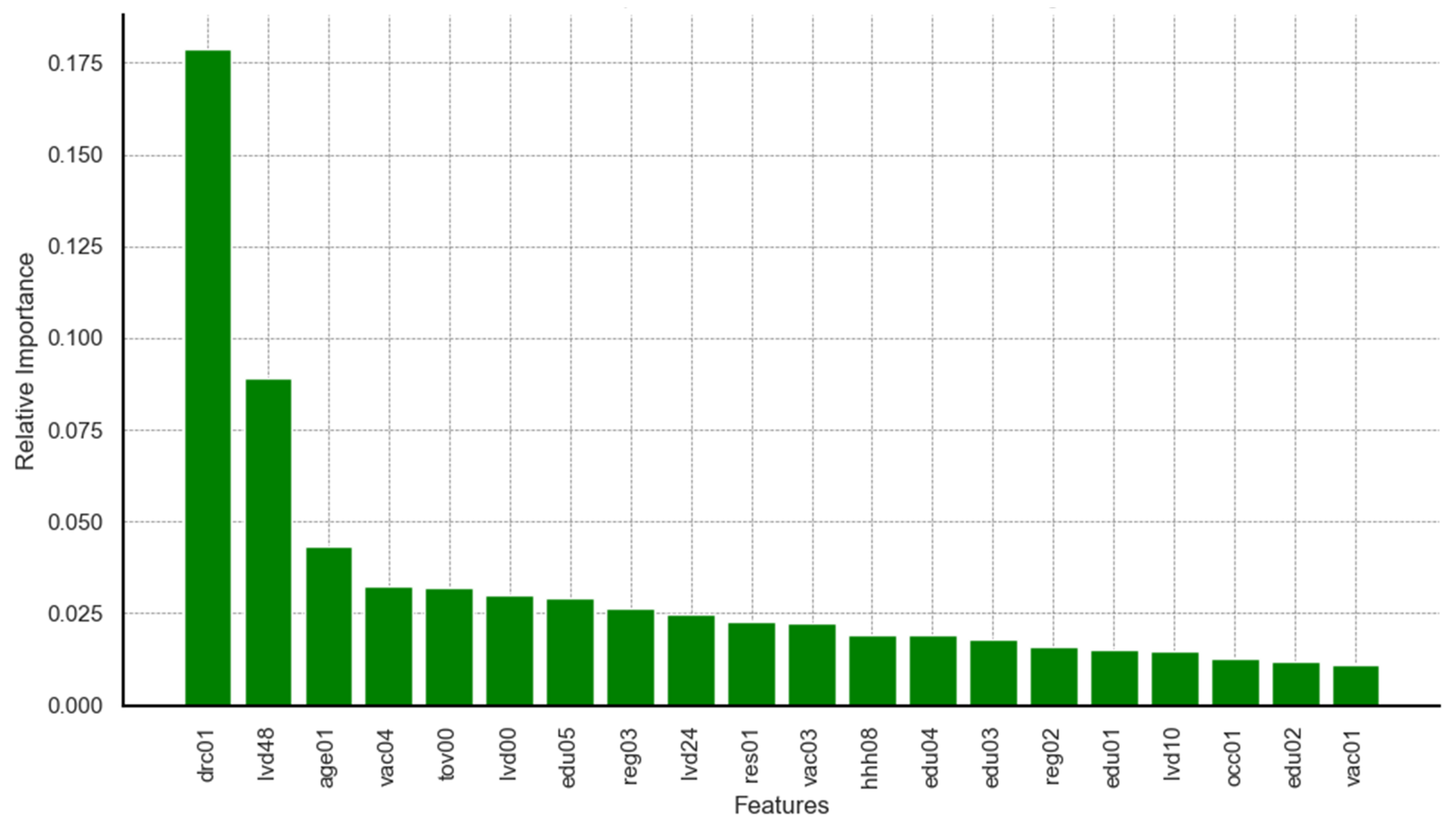
Limiting the results to the top 20 predictors identified by each model, relevant charts are presented in Figure A8, Figure A9 and Figure A10 in Appendix A. A map for feature code interpretation is provided in Table A2 in Appendix A. It can be seen from the results on feature importance that dimensions related to survey round, age of child, timeliness of vaccination at birth, and delayed vaccination were ranked among the top five predictors across all three models. Predictors such as maternal education and region of residence appeared, though not highly ranked, consistently among features within the top 20 across all models. Additional predictors identified by the highest performing models (RF and XGB) included dimensions on household wealth status, rural–urban residency, occupation, maternal hygiene and health practices, and birth seasonality.

4. Discussion

From the analysis of sample characteristics, we observed statistically significant differences in the distribution of defaulters across survey rounds (p < 0.001), with 62.5% of defaulters captured in the baseline and 84.1% of non-defaulters in the endline. There variations could be partly attributed to continuous maturity of the national EPI programme as well as the increased public efforts to improve childhood vaccination coverage during pilot implementation of the malaria vaccination. It is worth mentioning here that there were no major shifts in national vaccination policy or health system resource allocation between the two survey rounds.

The high performance observed in the RF, GBM, and XGB models is in line with assertions by Sibindi and colleagues [43] on the increasing essential role that ensemble decision tree classifiers are playing in solving classification problems. Ensemble methods like random forest and gradient boosting machines, as noted by Hu and colleagues [44], have a high capacity to manage non-linear relationships and prevent overfitting through random aggregation of many weaker learners. This trend diverges from the findings of Bediako and colleagues [25] when a comparison is made between the classical statistical logistic regression model and the ensemble random forest classifier. This, however, does not diminish the effectiveness of the logistic regression model, which reported significantly higher performance compared to the support vector machine during cross-validation. In addition, the effect of data size on model performance was apparent. We believe that the performance of the neural network model, although relatively high, was undermined by the lack of a more extensive dataset, which Çolak [45] found to be an essential requirement for neural networks during an experimental study on data size and neural network performance.

In terms of the key predictors identified, features identified across the three models included age of child, maternal education, and region of residence. These predictors correspond with prior research such as Bediako and colleagues [25] and Aheto, J. M. K. et al. [46], emphasizing the role of socio-demographic factors in vaccination adherence. The high-performing random forest model highly ranked other predictors such as household wealth status, which aligns with the works of Nantongo, B. A. et al. [12]. The importance of timely vaccine administration has not been a central focus in many machine learning studies on the risk of childhood vaccination default. However, in our analysis, it emerged as a significant predictor, possibly corroborating the works of Adetifa and colleagues [19], who suggested delayed vaccination as a key issue affecting childhood vaccination within the sub-Saharan African region.

Our findings contrast with those reported by Bediako and colleagues, who observed lower predictive performance in the ensembled machine learning model used. In

Table 15. A comparison with previous works on model performance.

Aspect	Bediako et al. [25]	Our Study
Original data size	643	13,724
Data enhancement	None	SMOTE Bootstrap resampling
Number of features	16	158
Feature engineering depth	One-hot encoding	One-hot encoding Aggregation Temporal feature transformations
Modelling techniques	Logistic regression Decision tree Random forest	Logistic regression Support vector machine Random forest Gradient boosting machine Extreme gradient boosting Artificial neural networks
Evaluation methods	Precision Recall F1 score accuracy ROC AUC	Precision Recall F1 score accuracy ROC AUC
Performance range	56–75%	77–95%

, we contrast our current work with previous work based on several key methodological differences that can explained model performance differences.

As seen in Table 15, our study used a much larger dataset (13,724 records vs. 643), applied multiple data enhancement techniques (SMOTE and bootstrap resampling), and incorporated diverse feature engineering strategies, including temporal encoding of vaccine delays and seasonality. In contrast, Bediako and colleagues relied on a smaller set of socio-demographic features and evaluated fewer algorithms. Our use of more diverse and sophisticated machine learning models also contributed to the higher rigour of the analysis, with AUC values as high as 95% compared to a maximum of 75% in the previous study. These results highlight the importance of data scale, extensive feature design, computational depth, and model diversity in improving the prediction of vaccination defaulters.

We acknowledge several limitations that may influence the outcomes of this study. First, this study relies on documented vaccination records as a proxy for vaccine receipt. This approach assumes that individuals without documented evidence of vaccine administration were classified as defaulters, which may not account for instances where vaccinations were administered but not recorded. As such, there is the possibility of vaccination coverage underestimation due to false classification of such children as defaulters. Also, the vaccination time window computations were performed with reference to the child’s date of birth rather than the date of consecutive vaccine schedules. As such, an earlier default which might have required real-world schedule adjustments may have staggered effects on how the timeliness of subsequent schedules was classified. In addition to this, there were several instances where the recorded vaccination dates varied across antigens within a specific window due to transcription errors. So, it would be inaccurate to definitively attribute all date deviations to genuine delays in administration. Secondly, the surveys analysed were conducted within the same geographic region over a 24-month period and so the possibility of data duplication cannot be entirely ruled out. With respect to the introduction of timely vaccination windows, we agree with [19] that continuous data representations would have been more informative compared to the binary vector indicators of delayed vaccination used. However, inaccuracies in the vaccination cards and paper-based hospital registries from which the survey data were extracted constrained the effectiveness of performing accurate continuous datapoint calculations on the length of vaccination timeliness. Also, while birth season emerged as a significant predictor of defaulting, this finding reflects an association rather than a confirmed causal relationship. Birth during the dry season may coincide with increased household mobility, reduced health service accessibility, or competing economic priorities, all of which may influence vaccination adherence. These potential confounders were not directly measured in the current dataset and may partially explain the observed relationship. These limitations should be considered when interpreting the findings of this study. For instance, associations between temporal features and vaccination default should be interpreted as a hypothesis-generating insight that highlights the need for further investigation into seasonal and vaccination timing factors affecting immunization uptake. Lastly, a key limitation of machine learning models lies in interpretability. Although these ensemble decision trees achieved high predictive performance, their complex structure reduces transparency in explaining individual predictions. As such, it is difficult to justify why a particular child is predicted as being at risk of defaulting. This complexity often limits their direct utility in real-world decision-making and resource use.

Despite the foregoing limitations, this study contributes to the growing body of evidence supporting the use of machine learning in public health interventions, particularly in predicting vaccination defaulters. The findings suggest that advanced analytical techniques, when applied to sufficiently large and well-prepared datasets, can enhance the precision and effectiveness of targeted interventions aimed at improving vaccination coverage. In terms of policy, this study has potential for real-world integration into Ghana’s public health system. Specifically, it could complement existing digital national platforms, such as the District Health Information Management System (DHIMS-2), to identify children at risk of defaulting from routine vaccination schedules, and inform interventions such as home visits, SMS reminders, or community mobilization. However, successful implementation would require validation in diverse settings and alignment with national health information policies.

5. Conclusions

This study explored the application of machine learning techniques to identify predictors of childhood vaccination defaulters from data that were collected from three administrative regions in Ghana, leveraging a relatively large dataset derived from multiple surveys. As such, the results may not fully capture the diversity of Ghana’s broader demographic, geographic, and health system contexts. The findings demonstrate the potential of machine learning, particularly ensemble methods like RF, GBM, and XGB models, in improving the prediction of vaccination defaulters compared to traditional statistical methods. The RF and XGB models reported the highest AUC (0.95) compared to all other models, with significant differences recorded against the GBM (p < 0.001) and ANN (p < 0.001) models. Key predictors of vaccination defaulting identified in this study include timely receipt of birth dose and week six vaccines, child’s age, household wealth index, health insurance coverage, residential location (urban vs. rural), and caregiver access to transportation. Future research should focus on expanding dataset sizes, incorporating additional contextual factors, and exploring hybrid models that combine the strengths of statistical and machine learning approaches. Such hybrid models could leverage statistical estimates such as confidence intervals or causal reference mechanisms for significance analysis and improved explainability in machine learning tasks.