Research and Experimental Verification of an Efficient Subframe Lightweighting Method Integrating SIMP Topology and Size Optimization

Abstract

Under the context of the dual-carbon policy, reducing energy consumption and emissions in automobiles has garnered significant attention, with automotive lightweighting being particularly important. This paper focuses on the lightweight design of automotive subframes, aiming to minimize weight while meeting performance requirements. Research has revealed that the original subframe allows further room for lightweighting and performance optimization. A topology optimization model was established using the Solid Isotropic Material with Penalization (SIMP) method and solved using the Method of Moving Asymptotes (MMA) algorithm. Integration of the SIMP method was achieved on the Abaqus-Matlab (2022x) platform via Python (3.11.0) and Matlab (R2022a) coding, forming an effective optimization framework. The optimization results provided clear load transfer paths, offering a theoretical basis for geometric model conversion. The subframe model was subsequently reconstructed in CATIA. Material redundancy was identified in the reconstructed subframe model, prompting secondary optimization. Multi-objective size optimization was conducted in OptiStruct, reducing the subframe’s mass from 33.73 kg to 17.84 kg, achieving a 47.1% weight reduction. Static stiffness and modal analyses performed in HyperMesh confirmed that results met all relevant standards. Modal testing revealed a minimal deviation of only −2.7% from the simulation results, validating the feasibility and reliability of the optimized design. This research demonstrates that combining topology optimization with size optimization can significantly reduce weight and enhance subframe performance, providing valuable support for future automotive component design.

1. Introduction

In modern automotive design, the performance of subframes directly influences vehicle handling stability, comfort, and safety. To achieve lightweighting and high performance, numerous researchers employ technologies such as Finite Element Analysis (FEA), topology optimization, and composite materials for subframe design optimization.

Ali et al. [1] utilized LS-DYNA to construct a subframe model for a Chevrolet vehicle, evaluating and optimizing the design under both normal driving and crash scenarios. Han et al. [2] introduced composite materials, discovering that they outperformed steel in stiffness, strength, and NVH (Noise, Vibration, Harshness) performance while reducing weight by half. Da’Quan et al. [3] employed ANSYS for topology optimization, enhancing the structural efficiency of side rails without increasing mass. Gosavi and Sinha et al. [4] improved frame performance through optimization of modal parameters; Han et al. [5] combined sensitivity assessment with FEA techniques to achieve structural lightweighting for heavy-duty trucks. Liao et al. [6] adopted the ICM hybrid modeling method, reducing subframe weight by 1.84 kg and increasing modal frequency by 10.2 Hz. Zhao [7] established a multi-body dynamics simulation system using the ADAMS platform to analyze force characteristics and refine the design. Ma et al. [8] integrated implicit parametric modeling with topology optimization, achieving a subframe weight reduction of 2.41 kg. Zhu [9] improved topology optimization methods to satisfy engineering constraints while enhancing performance. Jiang et al. [10] employed finite element techniques with inertia relief methods to investigate strength characteristics of the subframe, realizing a 9.9% weight reduction. Wang et al. [11] developed a bidirectional progressive structural topology optimization approach by integrating the ABAQUS-MATLAB platform. This methodology effectively addresses the limitations associated with the closed architecture of existing finite element software’s topology optimization modules, thereby enhancing both the flexibility and efficiency of the optimization process. The proposed method has exhibited significant advantages in practical engineering applications, offering a more effective solution for structural design.

In summary, existing research primarily focuses on finite element analysis, topology optimization, and composite material applications, but further improvements in comprehensive performance require continued exploration. This paper proposes an efficient and practical subframe design optimization methodology, aiming to provide new perspectives and references.

The technical roadmap centers on lightweight subframe design. After comparing multiple optimization platforms, Abaqus-Matlab was selected for implementing SIMP-based topology optimization. This innovation lies in applying this method to the conceptual design of the subframe. By extracting hard point loads from Adams-car and establishing an envelope volume model imported into the Abaqus-Matlab platform, optimal load transfer paths for the subframe were obtained. Based on these optimization results and overall packaging constraints, a framed subframe was reconstructed in CATIA. Preliminary static analysis indicated material redundancy, necessitating secondary optimization. Multi-objective size optimization was subsequently conducted in OptiStruct, with the final design validated through a combined simulation and experimental approach. This research establishes a theoretical foundation for lightweight subframe design while providing practical implications for automotive lightweighting strategies.

2. Materials and Methods

2.1. Finite Element Modeling of the Baseline Subframe

The baseline subframe material is SAPH440 steel, with its fundamental material properties detailed in

Table 1. Material parameters.

Material	Density (g/cm3)	Elastic Modulus (MPa)	Poisson’s Ratio	Yield Strength (MPa)
SAPH440	7.85	210,000	0.3	306

. The reference subframe for comparative design has a mass of 33.73 kg, and its finite element model is shown in Figure 1.

The areas indicated by the red arrows in Figure 1 are loading points, and there are four loading points. The white triangular area represents the fixed constraint points.

Figure 2 shows the unit quality information. According to the information in the figure, all information standards comply with industry standards. The following are the definitions and reasonable value ranges of each standard:

(1)

Max Size refers to the maximum side length or diameter of the cell, which is used to control the refinement degree of the grid. The selection of Max Size is based on the specific requirements of the model and does not exceed 1/20 of the feature size.

(2)

Aspect Ratio is the ratio of the length of the longest side to the length of the shortest side of a unit, which is used to measure the uniformity of the unit. Set value: The aspect ratio shall not exceed 5, and in the optimal case, it is close to 1. Set the value from 1 to 5 as the qualified standard.

(3)

Warpage is mainly used to evaluate the flatness of quadrilateral elements. Ideally, the quadrilateral elements should be completely located on one plane. Set value: In HyperMesh, a warpage of no more than 5% (i.e., 0.05) is considered a qualified standard.

(4)

Skew measures the degree to which an element deviates from its ideal shape. Quadrilateral: It is usually calculated based on the maximum deviation of the interior angles of the elements. Triangle: Calculated based on the ratio of the maximum interior angle to the minimum interior angle. The smaller the distortion value, the better the unit quality. Set the distortion value not to exceed 0.85.

(5)

The Jacobian is an important indicator for describing the degree of deformation of an element. It reflects the degree of deformation of an element from its ideal shape (such as a square or an equilateral triangle) to its actual shape. The ideal range of the Jacobian value is [0, 1]. The closer the value is to 1, the closer the unit shape is to the ideal state. Negative value: If the Jacobian value is negative, it indicates that the unit has been flipped, which is absolutely unacceptable and requires immediate correction. The setting value: A Jacobian value greater than 0.6 is considered a qualified standard.

(6)

Max Angle and Min Angle, respectively, refer to the maximum and minimum values among all the angles within the unit. Set the standard Max Angle Quad: The maximum angle should generally not exceed 135 degrees. Min Angle Quad: The minimum angle is generally not less than 45 degrees. Max Angle Tria: The maximum angle should generally not exceed 150 degrees. Min Angle Tria: The minimum angle should generally not be less than 15 degrees.

(7)

Taper is typically used to assess the shape quality of triangular elements, especially for non-equilateral triangles. The smaller the Taper value, the better the unit quality. Set a Taper value not exceeding 0.8 as the qualified standard.

The above is the quality information of the grid cells. According to these design standards, the divided grids were inspected. After modification, it can be seen from the figure that the quality of all these grids fully meets the standards and requirements for grid division.

As the structure of each component of the subframe is plate-shaped or hollow tubular, and its length and width are much greater than its thickness, the finite element model of the original subframe is established by drawing a grid from the drawing surface. The reference subframe finite element model has a total of 34,297 elements. The types of shell elements are mainly quadrilaterals, with a very small portion being triangles. There are 1398 triangular elements, and the proportion of triangular elements in the total number of shell elements is less than 5% as stipulated. The connection method of the subframe used in this article is mainly seam welding, while the rest of the parts are connected by bolts, etc. The shell element method is adopted to simulate the weld seam. Usually, 1.5 to 2.5 times the thickness of the connecting plate is selected to define the element thickness, which can more truly reflect the force state of the weld seam and has a relatively small impact on the overall stiffness. The RB2 element is adopted to simulate the weld connection. Finally, after the division is completed, the standardization of the overall model should be checked in accordance with the enterprise standards.

Both the loading points and the fixed constraint points adopt RB2 elements to simulate bolt connections. The simulated bolt connection is shown in Figure 3a. The simulated weld seam connection is shown in Figure 3b:

2.2. Subframe Load Extraction

As an important component of the automotive suspension system, the static force analysis of the subframe is of great significance for structural optimization and durability assessment. Based on ADAMS/Car, the static load of the subframe can be extracted through the static balance analysis method. Firstly, establish the subframe model and set reasonable constraint conditions to fix its installation points while allowing the suspension connection points to move freely. Subsequently, static loads are applied, including wheel loads, suspension forces and powertrain forces, to simulate the force conditions of the vehicle under different working conditions. Statics was solved by using ADAMS/Car to obtain the force data of each key part of the subframe. Finally, the reaction forces at the subframe installation points, the forces at the suspension connection points and the overall force distribution were extracted through the post-processing module, and the data were exported for further analysis. This method can effectively evaluate the force conditions of the subframe under static working conditions, providing a reference for structural optimization and lightweight design. The automotive suspension assembly model established in the ADAMS/Car standard mode is shown in Figure 4.

When constructing the subframe dynamic model in the initial stage, it is necessary to set the Marke reference points and define the force requirements of each joint part. Subsequently, extreme driving states such as braking, steering braking and acceleration were selected to measure the ground load of the tires. The multi-dimensional force data under these extreme conditions were imported into the model for static simulation, and finally the load values at the junction points were extracted. As shown in

Table 2. Static load of the lower swing arm connected on the left side.

Operating Condition	FX/N	FY/N	FZ/N
1	−120	−2479	−1498
2	−179	−8550	−1331
3	−249	−1248	−1430
4	−197	−8233	−1596
5	−120	−3060	−1496
6	−189	−85	−1368
7	−98	−1538	−1347
8	−211	−11,501	−2766
9	19	937	587
10	−97	−3395	−2210

Note: The above working conditions, in sequence, are as follows: static load working condition, double wheel runout working condition, longitudinal force working condition, lateral force working condition, forward acceleration working condition, forward braking working condition, backward braking working condition, right turn working condition, left turn working condition, braking + right turn working condition.

, the force conditions of some loading points at the connection of the left lower swing arm are presented. Among them, F_X, F_Y, and F_Z are the forces in the X, Y, and Z directions, respectively. The unit of force in the table is Newton, and the coordinate system adopted is the global coordinate system.

3. Performance Analysis of the Original Subframe

Strength Performance Analysis

Based on the hard point loads obtained from the above decomposition, the finite element model was loaded in the Hypermesh software. The steel grade used in the original subframe was SAPH440. For the above ten typical extreme working conditions, the stress distribution cloud diagrams obtained from the strength analysis are shown in Figure 5.

According to the simulation analysis results, the maximum stresses of the primary and rear subframes under ten working conditions are 115 MPa, 229 MPa, 245 MPa, 204 MPa, 126 MPa, 113 MPa, 99.6 MPa, 211 MPa, 144 MPa, and 131 MPa, respectively. None of them exceed the yield ultimate stress of 306 MPa of the materials used, which is in line with the enterprise standards. However, there is also an uneven stress distribution. Stress concentration occurs at the connection points with parts such as the lower control arm and the front beam tie rod, while the stress at the front crossbeam position is relatively small. It can be seen that there is still room for optimization in the original subframe structure.

4. Design Scheme of SIMP Method in the Abaqus-Matlab Topology Optimization Integration Framework

4.1. SIMP Optimization Algorithm

Taking the overall flexibility (strain energy) of the structure as the objective function and the artificially set final retained volume fraction of the material as the constraint condition, the topology optimization is carried out by using the variable density method based on the SIMP difference function. The specific mathematical model is constructed as follows [12]:

$$\mathrm{Find} X=\left(x_1,x_2,x_3\dots x_i\dots x_n\right)\in \mathrm{R}$$

(1)

$$\mathrm{Min} C=F^{\mathrm{T}}U=U^{\mathrm{T}}\mathrm{K}U={{\displaystyle \sum }}_{\mathrm{i}=1}^{\mathrm{n}}{\left(x_i\right)}^{\mathrm{p}}{\mathrm{u}}_{\mathrm{i}}^{\mathrm{T}}{\mathrm{k}}_0{u}_i$$

(2)

$$KU=F$$

(3)

$${\displaystyle \frac{V}{{\mathrm{V}}_0}}=f$$

(4)

$$0\le x_{min}\le x_i\le 1$$

(5)

In the analysis, the pseudo-density vector $X$ represents the element characteristics, $C$ flexibility reflects the structural performance, $F$ is the load vector, $U$ is the displacement vector, $\mathrm{K}$ is the structural stiffness matrix, ${\mathrm{k}}_0$ is the initial element stiffness matrix, $V$ is the optimized volume, $V_0$ is the initial volume of the structure, $f$ is the volume fraction, $x_i$ is the pseudo-density of element i, and p is the penalty factor. A coefficient affects the shape of the interpolation function, where $x_{min}$ is the lower limit of the element pseudo-density. To avoid the stiffness matrix being singular due to excessive material pores, the lower limit of the element pseudo-density is usually set as a positive number close to zero.

4.2. Variable Density Method Material Interpolation Model

The assumption of the variable density method is that the elastic modulus of the material can be expressed in the form of a function through the pseudo-density of the element. If the relative density of the small units in the structure is $x_i$, then the corresponding elastic modulus can be expressed as:

$$E_i=f\left(x_i\right){\mathrm{E}}_0\left(\mathrm{i}=1,2\dots \mathrm{n}\right)$$

(6)

Among them, $E_0$ is the elastic modulus of the material, and i represents the tiny unit.

The SIMP method is the most commonly used interpolation model in the variable density method. This interpolation model takes the pseudo-density of the element material with values ranging from 0 to 1 as the design variable. According to the basic concept of the variable density method, the interpolation function needs to have the following characteristics:

This function is continuous and defined within the interval (0, 1), and its range of values should approach either 0 or 1. For interpolation functions, having a definition within the (0, 1) interval is the basic condition for their existence, and the characteristic that the value range approaches 0 or 1 is conducive to efficiently screening out low-density units during material screening. The interpolation function constructed by the SIMP method is shown as follows:

$$\mathrm{SIMP}:f\left(x_i\right)=x_i^p$$

(7)

In the SIMP interpolation method, the penalty coefficient $p$ is a key variable, and its influence on the function shape is quite obvious. As shown in Figure 6, the characteristic curves of these two interpolation functions are presented when the penalty coefficients take different values.

In this interpolation algorithm, the variation of the regularization parameter directly determines the curve shape. When the parameter value increases, the constraint effect intensifies, the function tends to a two-pole distribution, and the number of samples in the middle region significantly decreases. As the penalty factor increases, more units will approach zero, which makes the model matrix tend to be singular and further affects convergence and iterative operations. This does not conform to the actual engineering situation. Therefore, the penalty factor should not be too high. Generally, taking 3 is more appropriate.

From the above chart and analysis, it can be seen that topological optimization technology adopts the principle of variable density, introducing the variability of material density, thereby establishing the connection between the pseudo-density of structural elements and the elastic modulus. Transform the discrete problem of the two states of “existence or non-existence” into a continuous problem with a value range from 0 to 1.

4.3. Numerical Algorithm for Solving Topology Optimization

When dealing with highly nonlinear problems such as topology optimization, the convex programming method has become an ideal solution tool. At present, the Moving Asymptote method (MMA), as a representative algorithm in this field [13], has developed to a mature stage. This method is based on Taylor series expansion. By ingeniously applying sensitivity data and function values, it decomposes complex nonlinear problems into multiple manageable sub-problems. This algorithm has excellent convergence characteristics and low requirements for initial values, making it particularly suitable for solving nonlinear problems. In this study, the Moving asymptote method (MMA) is adopted for optimization calculation. The key lies in using the moving asymptote technique to approximately transform the non-convex functions within the design region into convex functions, thereby gradually constructing sub-problems and iteratively solving them to ultimately meet the convergence conditions. The mathematical approximation formula of MMA can be described as follows:

$${\tilde{f}}_j^n\left(x\right)=r_j^n+{{\displaystyle \sum }}_{i=1}^l\left({\displaystyle \frac{P_{ij}^n}{U_i^n-x_i}}+{\displaystyle \frac{q_{ij}^n}{x_i-L_i^n}}\right)$$

(8)

$$P_{ij}^n=\left\{\begin{array}{c}\hfill {\left({\mathrm{G}}_i^n-x_i^n\right)}^2{\displaystyle \frac{\partial f_j\left(x^n\right)}{\partial x_i}},{\displaystyle \frac{\partial f_j\left(x_i^n\right)}{\partial x_i}}<0\hfill \\ \hfill \\ 0 ,{\displaystyle \frac{\partial f_j\left(x_i^n\right)}{\partial x_i}}\le 0\hfill \end{array}\right.$$

(9)

$$q_{ij}^n=\left\{\begin{array}{l} 0 , {\displaystyle \frac{\partial f_j\left(x_i^n\right)}{\partial x_i}}\ge 0\hfill \\ \hfill \\ -{\left(x_i^n-L_i^n\right)}^2{\displaystyle \frac{\partial f_j\left(x^n\right)}{\partial x_i}},{\displaystyle \frac{\partial f_j\left(x_i^n\right)}{\partial x_i}}<0\hfill \end{array}\right.$$

(10)

$$r_j^n=f_j\left(x^n\right)-{{\displaystyle \sum }}_{i=1}^l\left({\displaystyle \frac{p_{ij}^n}{U_i^n-x_i^n}}+{\displaystyle \frac{q_{ij}^n}{x_i^n-L_i^n}}\right)\left(j=0,1\cdots ,j+1;i=1,2\cdots n\right)$$

(11)

Here, ${\tilde{f}}_j^n\left(x\right)$ represents an approximate function of the original function $f\left(x\right)$, $n$ is the number of iteration steps, and $L_i^n$ and ${\mathrm{G}}_i^n$ are the asymptotes for left and right movement, mainly regulating convexity. $P_{ij}^n$ and $q_{ij}^n$ are the left and right asymptotes and the sensitivity of the design unit is determined, $r_j^n$ is an undetermined parameter, and $x^n$ is the current design unit.

4.4. Advantages of the Abaqus-Matlab Integration Framework

This study combines the finite element analysis capability of Abaqus and the efficient computing characteristics of Matlab to achieve the integration of the SIMP method in the ABAQUS-MATLAB environment for the topological optimization of subframes. It is difficult to precisely define complex optimization models using Matlab alone, while using Abaqus alone is limited by the flexibility of its built-in optimization algorithms. Therefore, combining the two can fully leverage the powerful analytical capabilities of Abaqus and the rapid computing capabilities of Matlab to enhance optimization efficiency.

The specific advantages of the Abaqus-Matlab integrated framework are as follows:

• Adapt to complex design requirements: Abaqus can conduct various working condition analyses, while Matlab controls the optimization process to ensure that the design meets all kinds of conditions.
• Flexible optimization algorithm design: Matlab offers a flexible programming environment that allows for the customization of optimization algorithm parameters, such as penalty factors and filter radii. Combined with the simulation support of Abaqus, multi-objective optimization and complex constraint condition setting can be achieved.
• Enhance optimization efficiency: Although the finite element solution of Abaqus is time-consuming, Matlab can quickly process gradient information and sensitivity analysis. Matlab is seamlessly integrated with Abaqus, simplifying the optimization process, accelerating the adjustment of material distribution, and enhancing work efficiency.

4.5. Abaqus-Matlab Interface Scheme

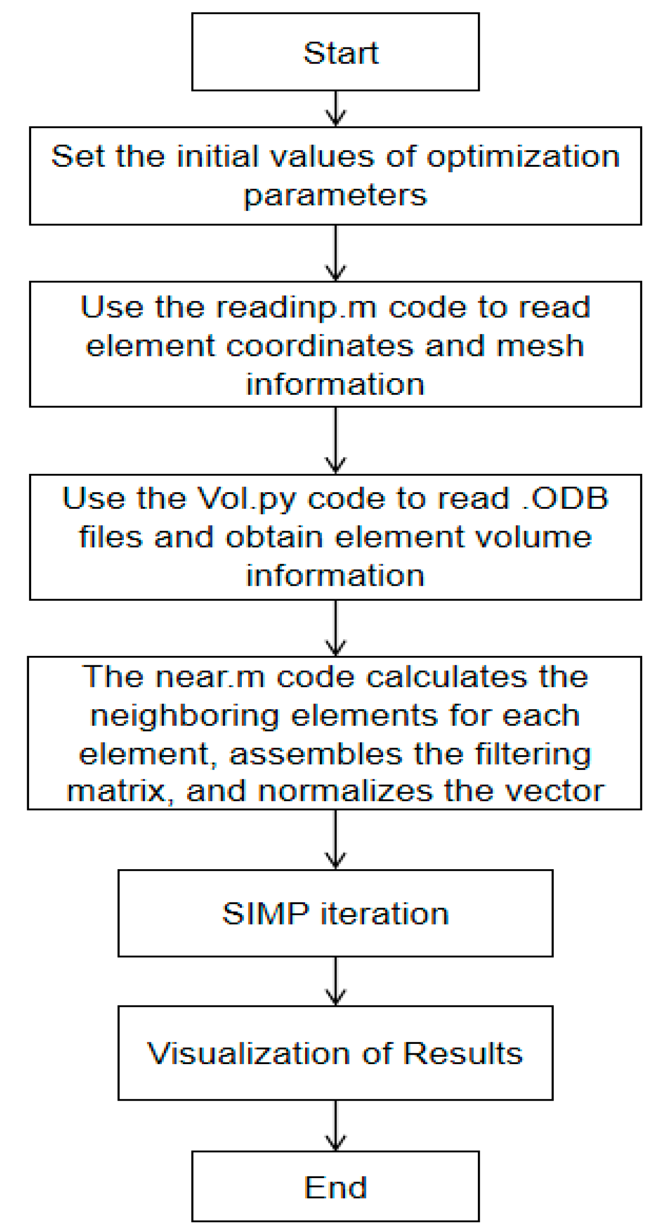
The SIMP method is based on the continuum topology optimization theory, and its core is an iterative computing process. When formulating the overall plan, a complete circular mechanism needs to be established. In view of the data interaction requirements between Abaqus as a finite element analysis tool and Matlab as a mathematical operation platform, system compatibility becomes a key consideration factor. Based on the above analysis, the scheme design is shown in Figure 7.

Firstly, the basic finite element model is constructed through Abaqus. After generating the inp format file, it is transferred to the Matlab environment to implement the SIMP algorithm operation. During the iterative process of topology optimization in Matlab, there is no need for manual operation of Abaqus for finite element analysis. The calculation can be completed simply by relying on the core command-line call function of Abaqus. In the Abaqus-Matlab platform, the SIMP method is integrated through the main functions of Matlab. The calculation process mainly includes the following steps. Firstly, the initial model data is submitted to Abaqus through the inp file for finite element solution. Then, the data is extracted and analyzed in Matlab. The SIMP algorithm is used for structural optimization and the updated inp file is generated. Finally, through iterative calculation until the convergence standard is reached, the final optimization scheme is output.

The key to building the joint platform of Abaqus and Matlab lies in establishing the data interaction channel. This platform realizes interconnection by extracting the calculation results of Abaqus through Matlab. Abaqus saves the analysis data to the document, and Matlab acquires the required information by reading the document. The inp file plays a crucial bridging role between the Abaqus/CAE preprocessing module and the Standard/Explicit solver, and is processed by the solver as the core analysis object. By transferring the inp file to the Abaqus/CAE core, Matlab realizes the platform connection of finite element analysis, providing the necessary data interface for the joint simulation of Abaqus-Matlab. The data interaction between Abaqus and Matlab is accomplished by parsing the odb file to transfer the finite element calculation results.

4.6. Multi-Condition Optimization Design

In multi-condition topology optimization, the optimization results of each condition often differ, leading to conflicts during multi-objective optimization. To reconcile the conflicts of goals and integrate elements such as dimensions, weights and orders of magnitude, researchers often employ the compromise programming method to handle such difficult problems. This method can simplify complex multi-objective problems, and its calculation formula is as follows:

$$\min \left\{{\left[{{\displaystyle \sum }}_{i=1}^k{\lambda }_i^P{\left(f_i\left(x\right)-y_i^0\right)}^p\right]}^{{\displaystyle \frac{1}{p}}}\right\}$$

(12)

$$\mathsf{\Lambda }=\left\{\lambda \in R^k\mid \lambda \ge 0,{{\displaystyle \sum }}_{i=1}^k{\lambda }_i=1\right\}$$

(13)

In the formula, $f_i\left(x\right)$ represents the i-th sub-objective, $y_i^0$ is the optimal solution of the i-th objective function, and p ∈ [1, ∞). When the value of p varies, the formula is endowed with different practical meanings. This study focuses on improving the performance of subframe components and transforms the structural stiffness optimization problem into the solution of minimizing flexibility. Taking the minimum unit strain energy as the objective function, combined with the volume ratio and stress distribution constraints, and using the multi-objective optimization method, a multi-condition topology optimization design model was established:

$$\begin{array}{c}\hfill \min \mathrm{C}\left(\mathsf{\rho }\right)={\left\{{{\displaystyle \sum }}_{\mathrm{k}=1}^{\mathrm{m}}{\mathsf{\omega }}_{\mathrm{k}}^{\mathrm{q}}{\left[{\displaystyle \frac{\left({\mathrm{C}}_{\mathrm{k}}\left(\mathsf{\rho }\right)-{\mathrm{C}}_{\mathrm{k}}^{\min }\right)}{\left({\mathrm{C}}_{\mathrm{k}}^{\max }-{\mathrm{C}}_{\mathrm{k}}^{\min }\right)}}\right]}^{\mathrm{q}}\right\}}^{{\displaystyle \frac{1}{\mathrm{q}}}}\hfill \\ \mathrm{s}.\mathrm{t}.\left\{\begin{array}{ll}{\displaystyle \frac{\mathrm{V}\left(\mathsf{\rho }\right)}{{\mathrm{V}}_0}}\le \mathrm{f}\hfill & \hfill \\ {\mathsf{\sigma }}_{\mathrm{k}}\le \left[\mathsf{\sigma }\right]\hfill & \hfill \end{array}\right.\hfill \end{array}$$

(14)

Here, $\rho$ represents the density of the material; $m$ represents the number of load conditions ($m=6$); ${\omega }_k$ is the weight coefficient of the kth working condition; $q$ is the penalty factor ($q=2$); $C_k\left(\rho \right)$ is the total strain energy function of the unit under the load condition. $C_k^{max}$ and ${\mathrm{C}}_{\mathrm{k}}^{\min }$ are, respectively, the maximum and minimum values of the total strain energy function of the structure under the kth load condition; $V\left(\rho \right)$ is the optimized effective volume; $V_0$ is the initial volume; $f$ is the volume fraction limit value; ${\sigma }_k$ is the maximum stress value; $\left[\sigma \right]$ is the allowable stress of the material.

In the multi-condition structural optimization design, determining the weight coefficients of each condition is the current research focus. At present, there is still a lack of systematic investigations on the frequency of vehicle usage under extreme conditions. Coupled with the diverse design requirements of different vehicle models, there are differences in the attention paid to each condition. Therefore, it is necessary to conduct a comprehensive assessment of the working condition weights by combining literature and design practice. Generally, the setting of weights needs to take into account the degree of mechanical influence and the actual probability of occurrence under working conditions. The specific settings are shown in

Table 3. Weight settings for each working condition.

Number	Working Condition Name	Degree of Importance	Weight Setting
1	Static load working condition	General	0.08
2	Double wheel runout working condition	More important	0.1
3	Longitudinal force working condition	General	0.08
4	Lateral force working condition	General	0.08
5	Forward acceleration working condition	More important	0.1
6	Forward braking working condition	More important	0.1
7	Backward braking working condition	General	0.08
8	Right turn working condition	Very important	0.2
9	Left turn working condition	More important	0.1
10	Braking + right turn working condition	General	0.08

.

4.7. Subframe Envelope Creation and Topology Optimization

4.7.1. Creation of the Subframe Envelope

When establishing the design space, to ensure the reliability of the topological optimization results, a series of design specifications and principles must be followed, among which the influence of the model is also a factor that we must consider. According to these requirements, the following points should be specifically achieved [14,15]:

According to the requirements of the plan, precisely locate the key parts of the structure to ensure that the loading points and constraint points are consistent with the original subframe. The connection methods between the vehicle body and components such as the suspension should be scientifically selected to ensure the stability and reliability of the optimization effect. When arranging the space, it is necessary to maximize it as much as possible while ensuring that it does not interfere with or affect the movement of surrounding components. In the geometric modeling process of the subframe, a 5 mm specification hexahedral mesh is adopted for the preliminary processing to optimize the design space analysis. To ensure the feasibility of the manufacturing process, a scientific division of the design area was implemented. In terms of materials, SAPH440 steel is selected as the structural material for automobiles. Its basic performance parameters are detailed in Table 1.

According to the above principles, the finite element model of the subframe envelope is shown in Figure 8. The finite element model of the subframe envelope has a length of 1000 mm (the long side is in the x direction), a width of 900 mm (the wide side is in the z direction), and a height of 150 mm (the height is in the y direction). The number of nodes is 117,845, and the number of grids is 105,588. The white parts in the figure represent the fixed constraint points and the load application points. The blue part is the design area.

4.7.2. The Subframe Envelope Is Imported into the Abaqus-Matlab Optimization Platform Based on SIMP

First, set the working path of Abaqus and that of Matlab in the same folder. After importing the model to be optimized into Abaqus, you only need to manually use Abaqus for the first finite element analysis. There is no need to manually operate Abaqus for the subsequent optimization process. At this point, the finite element result file appears in the working path of Matlab. It is only necessary to start Matlab to extract the information in each result file of the finite element and modify the design variables. After each iteration of Matlab, new design variables are generated. Matlab calls Abaqus to conduct finite element analysis on the new design variables (Figure 9).

4.7.3. Multi-Condition Optimization Results of the Subframe

After 150 rounds of iterations, the model diagram in Figure 8 was optimized to be as shown in Figure 10. Figure 10 shows the topological optimization structure of the subframe with a relative density exceeding 0.6, that is, the result of the optimization of the subframe topological space model. Based on the analysis of the subframe category and the optimization results, it can be determined that it is the prototype of the full-frame subframe, and this prototype represents the force transmission path of the full-frame subframe. Figure 11 presents the iterative curve during the optimization process. It can be clearly seen that it tends to level off after 150 iterations, indicating that a very good effect has been achieved after 150 iterations.

Through topology optimization technology, the design scheme adopting hollow structure was determined. Based on maintaining the original subframe layout, this scheme has rationally optimized the structural form and continues to use the plate and shell stamping process to construct the main frame. In the optimization process considering various working conditions, production limiting factors are introduced to ensure a more balanced material distribution and a more distinct structural contour, providing a more practical guiding basis for engineering design.

5. Model Reconstruction and Secondary Optimization

5.1. Model Reconstruction

Based on the optimization results of the subframe force transmission path obtained from topological optimization and the overall layout requirements of the actual application of the subframe as a reference, the subframe model after the first optimization is re-established. The details of this subframe are partially based on the original subframe of the same vehicle model, and the main part is modeled according to the topological optimization results. Draw the subframe model in the CATIA software and export it. The following are the three views of the subframe as shown in Figure 12. The dimensions of each component are precisely marked in the figure. In the sub-vehicle drawing, A represents the rear crossbeam, B represents the front crossbeam, C represents the left and right vertical beams, and D represents the lower swing arm mounting plate.

One end of the lower control arm mounting plate D of the subframe is installed on the upper plate of the rear crossbeam, and the other end is coordinated with the lower plate of the rear crossbeam. One end of the lower control arm is connected by bolts to restrict the movement of the lower control arm. The vertical beams C on the left and right sides of the subframe serve to connect the front and rear crossbeams and are also responsible for connecting the front tie rods. The front crossbeam B bears less force and is installed at the front of the car, hence the name “front crossbeam”. There are two fixed constraints on each side. The width of the rear crossbeam A is wider than that of the front crossbeam, only because the lower swing arm and the lower swing arm mounting plate are both connected to this, and there are two fixed constraints on each side.

5.2. Lightweight Design of Subframe Based on OptiStruct

The main technical approach to lightweight design is structural optimization, which mainly includes topology optimization, shape optimization and size optimization. The transmission path of the subframe force was obtained through the completed subframe topology optimization. Relying on the completed model reconstruction, for the further lightweight design of the subframe, to increase the vehicle’s driving range and reduce energy consumption, further optimize the subframe.

By applying the size optimization technology of Optistruct, weight reduction optimization is achieved in the subframe design stage. Parameter adjustment technology, also known as size optimization method, focuses on finely adjusting various parameters of the three-dimensional model without changing the mesh structure, in order to achieve size optimization of the finite element model of mechanical components, such as precise control of plate thickness. This method is dedicated to achieving the lightweight design of the subframe to the greatest extent within the limitations of existing materials and manufacturing processes [16,17].

The relevant parameters for subframe size optimization are:

Objective function:

$$V_{min}\left(x_1,x_2,x_3,x_4,x_5\right),f_{max1}\left(x_1,x_2,x_3,x_4,x_5\right)$$

(15)

Constraint conditions:

$$\delta \le 306 \mathrm{MPa}$$

$$Y\le 1 \mathrm{mm}$$

(16)

$$f_1\ge 100 \mathrm{Hz}$$

Design variable:

$$1 \mathrm{mm}\le x_1,x_2,x_3,x_4,x_5\le 5 \mathrm{mm}$$

(17)

In the formula, $V$ represents the volume of the subframe; $\delta$ represents the subframe stress; Y represents the maximum deformation of the subframe; $x_1$ represents the thickness of the front crossbeam of the subframe; $x_2$ indicates the thickness of the rear crossbeam of the subframe; $x_3$ represents the thickness of the side beams of the subframe. $x_4$ represents the thickness of the subframe pipe string; $x_5$ is the connection plate of the lower swing arm.

The study was constructed using SAPH440 material. It was assumed that the density distribution was balanced and the weight of the subframe was positively correlated with its volume. Based on this, volume reduction is taken as the core goal of the optimized design. The subframe mode needs to avoid the road excitation frequency and the engine excitation frequency. Then, the maximum frequency of the first-order mode is set as the second objective function. If the yield strength of SAPH440 material is 306 Mpa, then the stress under the constraint condition needs to be less than 306 Mpa. The other first-order mode needs to avoid the engine frequency and the road excitation frequency. Therefore, the range of the first-order mode is set to be greater than 80 Hz. When designing the subframe, the deformation is required to be less than 1 mm. Set the thickness of each part of the subframe as the design variable of the subframe. Meanwhile, set the convergence tolerance at 0.5%. When choosing design variables, consider taking the thickness of the side beams of the subframe, the front crossbeam, the rear crossbeam, the lower swing arm connection plate and the pipe string as the design variables for achieving lightweight. These ten working conditions are selected as the reference conditions for strength constraints and stiffness constraints.

After the secondary optimization, the subframe is shown in Figure 13. The wall thickness of the left and right vertical beams is 3.3 mm, the thickness of the front crossbeam and pipe string is 1.3 mm, the thickness of the rear crossbeam is 1.6 mm, and the wall thickness of the lower swing arm mounting plate is 3.6 mm. You can view it by opening mass calc in the home page Tool in Hypermesh. Figure 11 shows the optimized quality.

5.3. Simulation Analysis and Experimental Verification of the Subframe After Secondary Optimization

5.3.1. Modal Analysis Results

When conducting free mode analysis on the subframe, to achieve this analysis, Hypermesh, a convenient commercial software, was used for modeling and analysis. The optimized modal analysis data will detail the vibration characteristics of the subframe and further verify the dynamic performance of the structure. For details, please refer to

Table 4. Modal analysis results of the first three subframes.

Mode Number	Natural Frequency (Hz)	Mode Shape Description
1	104.8	Torsional vibration
2	153.3	Bending Vibration
3	181.2	Bending Vibration

, and its vibration mode characteristics are shown in Figure 14.

5.3.2. Subframe Modal Test

To verify the accuracy of the simulation analysis, in this study, the rear subframe was inspected through modal tests. Based on the limitations of the experimental conditions, a specific subframe was selected for modal testing and simulation comparison. In the early stage of the experiment, structural feature points were selected for signal collection, and then external forces were applied through excitation equipment or impact hammers. Due to the simple operation and rapid response of the hammering method, the PCB force hammer was selected as the excitation tool in this study. When operating, it is necessary to ensure that the tapping direction is orthogonal to the excitation point, the force should be stable and moderate, and the interval time should be reasonably arranged. The installation of sensors can refer to the specifications, with a focus on deployment at the junctions of components, key excitation areas, and the core parts of the research object. At the same time, it is necessary to avoid the node positions of each mode [18,19].

To improve the test accuracy, five hammering operations were carried out at each excitation point and sensors were installed. After the experiment was completed, the collected data was processed by using the signal analysis system. Figure 15 shows the modal test process of the force hammer.

In this experiment, LMS Mobile SCM05 was used for signal analysis. Figure 16 shows the steps of modal detection. The input force signal is converted into the excitation self-spectrum ${\mathcal{S}}_{\mathrm{FF}}\left(\mathsf{\omega }\right)$, and the acceleration signal is converted into the response self-spectrum ${\mathrm{S}}_{\mathrm{XX}}\left(\mathsf{\omega }\right)$. The correlation between them is represented by cross-spectrum ${\mathcal{S}}_{\mathrm{FX}}\left(\mathsf{\omega }\right)$. The calculation formulas of the system frequency response function $H\left(\omega \right)$ and the coherence coefficient ${\gamma }_{FX}^2\left(\omega \right)$ are as follows [20,21]:

$$\begin{array}{rr}\hfill H\left(\omega \right)& ={\displaystyle \frac{{\mathrm{S}}_{XX}\left(\omega \right)}{{\mathrm{S}}_{FX}\left(\omega \right)}}\hfill \\ \hfill {\gamma }_{FX}^2\left(\omega \right)& \hfill ={\displaystyle \frac{{\left|{\mathrm{S}}_{FX}\left(\omega \right)\right|}^2}{{\mathrm{S}}_{XX}\left(\omega \right){\mathrm{S}}_{FF}\left(\omega \right)}}\end{array}$$

(18)

To eliminate invalid data caused by experimental errors, the signal coherence needs to be calculated before analysis. Usually, 0.8 is taken as the threshold to eliminate the data that do not conform to the linear relationship. After frequency response fitting processing, the comprehensive FRF was obtained. For details, please refer to Figure 17.

Modal analysis was carried out with the aid of Hypermesh, and then the first three orders of free modal frequencies and vibration modes of the optimized subframe were obtained. It can be seen in

Table 5. Comparison of simulation and experiment.

Mode Number	Test Frequency (Hz)	Simulation Frequency (Hz)	Error (%)
1	102.54	104.8	2.2
2	157.7	153.3	−2.7
3	179.3	181.2	1

that the maximum error between the two is −2.7%, which meets the engineering requirements. The accuracy of the finite element modeling was verified. In terms of modal performance, the design standards and requirements have been met.

5.4. Simulation Verification of Subframe Strength

After the design stage is completed, statics research is carried out to test whether the functional characteristics of the front subframe meet the requirements. When the damping effect and inertial effect are ignored, the structural load can be simplified to static load, and then its displacement and stress distribution can be investigated. This research method is called static analysis. With the help of this method, it is possible to determine whether the material stress exceeds its limit value, thereby evaluating the reliability of the structure. By applying the fourth strength criterion [22] combined with the von Mises stress theory [23], we evaluated the mechanical properties of the front subframe. By constructing a finite element analysis model and applying corresponding constraint conditions, the numerical simulation was completed using the OptiStruct (2022) computing platform. After the operation is completed, the operation results are organized. The stress cloud diagram of the subframe after secondary optimization is shown in Figure 18.

The stress cloud diagrams of the above 10 working conditions can be obtained, and all operating states have reached the expected indicators. In the right-turn scenario, the peak stress endured by the subframe is 262 MPa. This value is much lower than the yield limit of 306 MPa of SAPH440 material, indicating that the structural design fully meets the strength requirements.

5.5. Simulation Verification of Subframe Stiffness

Figure 19 shows the displacement cloud diagram of the subframe under ten working conditions. From the stress cloud diagram shown in Figure 19, it can be seen that the maximum displacement of the subframe when it is in the right-turning working condition is 0.92 mm. The displacement value of the subframe is 1 mm lower than the required maximum displacement value, and the stiffness meets the standard requirements.

6. Conclusions

This study aims at the lightweight design problem of automotive subframes and proposes a multi-stage optimization method based on the Abaqus-Matlab co-simulation platform. Through a closed-loop optimization process of topology optimization–size optimization–experimental verification, the performance of the subframe structure has been significantly improved and the lightweight goal has been efficiently achieved. The main research conclusions are as follows:

(1)

Platform innovation: The Abaqus-Matlab integrated optimization platform utilized, through the SIMP method and two-way data interaction mechanism, offers greater flexibility. After building this optimization platform, you can customize optimization algorithms on it according to specific needs.

(2)

Lightweighting achievements: The optimal force flow transmission path of the subframe was clarified through topological optimization, and the thickness parameters of key components (such as 3.3 mm for side beams, 1.3 mm for front crossbeams, etc.) were determined in combination with parametric size optimization. The final mass was reduced by 47.1% (33.73 kg → 17.84 kg), significantly reducing material redundancy while ensuring structural integrity.

(3)

Performance verification results: Static analysis shows that the maximum von Mises stress of the optimized subframe is 262 MPa, which is lower than the yield strength of the material (306 MPa). The maximum displacement is 0.92 mm, meeting the design threshold (<1 mm). The maximum relative error between the modal experiment and the simulation results was controlled within 2.7%, verifying the reliability of the optimization scheme.

The multi-stage optimization method proposed in this research has established a standardized technical process for the lightweight design of vehicle chassis structures. Its platform integration strategy is universal and can be extended to the optimization design field of various mechanical structures. Subsequent research will focus on the coupling optimization of multiple physical fields (structure–acoustic–thermodynamics) to enhance the performance robustness of structures under complex dynamic working conditions.