Accelerated Tensor Robust Principal Component Analysis via Factorized Tensor Norm Minimization

Abstract

In this paper, we aim to develop an efficient algorithm for the solving Tensor Robust Principal Component Analysis (TRPCA) problem, which focuses on obtaining a low-rank approximation of a tensor by separating sparse and impulse noise. A common approach is to minimize the convex surrogate of the tensor rank by shrinking its singular values. Due to the existence of various definitions of tensor ranks and their corresponding convex surrogates, numerous studies have explored optimal solutions under different formulations. However, many of these approaches suffer from computational inefficiency primarily due to the repeated use of tensor singular value decomposition in each iteration. To address this issue, we propose a novel TRPCA algorithm that introduces a new convex relaxation for the tensor norm and computes low-rank approximation more efficiently. Specifically, we adopt the tensor average rank and tensor nuclear norm, and further relax the tensor nuclear norm into a sum of the tensor Frobenius norms of the factor tensors. By alternating updates of the truncated factor tensors, our algorithm achieves efficient use of computational resources. Experimental results demonstrate that our algorithm achieves significantly faster performance than existing reference methods known for efficient computation while maintaining high accuracy in recovering low-rank tensors for applications such as color image recovery and background subtraction.

1. Introduction

Robust principal component analysis (RPCA) has been extensively studied to address the issue of extreme outliers contained in data, which causes significant degradation of the performance when applying classical principal component analysis [1]. Specifically, RPCA aims to separate outliers from the true data by reconstructing a low-rank matrix $L\in {\mathbf{R}}^{m\times n}$ from an observed matrix X, which is contaminated by sparse noise S of arbitrary magnitude, such that

$$X=L+S.$$

(1)

This RPCA model arises in numerous real-world applications, including image denoising, video background subtraction, subspace clustering, or feature selection in bioinformatics [2,3,4,5,6]. However, identifying the locations of sparse noise, i.e., the nonzero entries of S, is often challenging. Under the assumptions that L is low-rank and S is sufficiently sparse, it has been shown that one can accurately recover L by solving the following convex problem:

$${\min \parallel L\parallel }_{*}+\lambda {\parallel S\parallel }_1,\mathrm{s}.\mathrm{t}.X=L+S,$$

(2)

where ${\parallel ·\parallel }_{*}$ denotes the nuclear norm, ${\parallel ·\parallel }_1$ denotes the ${\mathit{l}}_1$ norm, and $\lambda$ is a regularization parameter [1]. A typical algorithm for solving the problem (2) is to apply singular value thresholding, which modifies the singular values of a matrix by applying a threshold operator [7]. However, as the data structure become increasingly complex, the matrix representation may no longer be sufficient for capturing the intricacies of real-world data. Since tensors can represent higher-order data while preserving spatio-temporal and multi-dimensional correlations, it is natural to extend RPCA to tensor setting. This motivates the extension of the RPCA model in (2) to the tensor RPCA (TRPCA) formulation, where the input is an n-th order tensor $\mathcal{X}\in {\mathbf{R}}^{I_1\times \dots \times I_n}$. The optimization problem of TRPCA is formulated as follows:

$${\min \left|\right|\mathcal{L}\left|\right|}_{*}+{\lambda \left|\right|\mathcal{S}\left|\right|}_1,\mathrm{s}.\mathrm{t}.\mathcal{X}=\mathcal{L}+\mathcal{S},$$

(3)

where $\mathcal{L}$ denotes a low-rank tensor, $\mathcal{S}$ is a sparse tensor, and $\lambda$ is a regularization parameter. However, this extension introduces new challenges, particularly due to the lack of a unified definition of tensor rank and tensor nuclear norm, unlike in the matrix case. For example, under Canonical Polyadic Decomposition (CPD), the tensor rank is defined as the minimum number of rank-1 tensors whose sum reconstructs the given tensor [8]. However the rank minimization problem with CP rank is generally NP-hard [9]. Another widely used definition is the Tucker rank, which consists of a tuple of ranks obtained by unfolding the tensor along each mode. Its convex surrogate can be formulated by summing the nuclear norms of the mode-wide unfoldings, leveraging ideas from matrix convex optimization [10]. More recently, tensor singular value decomposition (T-SVD) and tensor–tensor product (T-product) frameworks introduced by Kilmer et al. [11] led to definitions such as tensor multi-rank and tensor tubal rank. These ranks provide a more structured and compact representation of tensors and avoid the loss of structural information that typically occurs during tensor matricization. They are particularly useful for preserving the inherent low-rank structure in tensor data. Nevertheless, it should be noted that computing the T-SVD-based tensor ranks can be computationally demanding as the size of the tensor increases.

In this paper, we propose a novel and computationally efficient TRPCA algorithm based on tensor average rank minimization. Specifically, our main contribution is the further relaxation of the tensor nuclear norm—a convex envelope of the tensor average norm defined in (3)—into an optimization problem involving the sum of Frobenius norms of factor tensors. By alternatingly updating the truncated factor tensors from a given tensor, our method significantly improves computational efficiency while maintaining competitive reconstruction accuracy on real-world data compared to existing TRPCA algorithms. The remainder of this paper is organized as follows. In Section 2 we define the notations and preliminaries used throughout this paper. Section 3 introduces well-known TRPCA methods. In Section 4, we present our proposed TRPCA algorithm based on tensor average rank. Section 5 provides experimental results on real-world images and video sequences. Finally, Section 6 concludes this paper.

2. Notations and Preliminaries

We first summarize the symbols and terminologies consistently used throughout this paper. Capital calligraphy letters, e.g., $\mathcal{A}$, and capital letters, e.g., A, are used to denote tensors and matrices, respectively. Boldface lowercase letters, e.g., $\mathbf{a}$, and lowercase letters a represent vectors and scalars, respectively. For a third-order tensor $\mathcal{A}$, we adopt MATLAB-style notation: $\mathcal{A}(i,:,:),\mathcal{A}(:,i,:)$, and $\mathcal{A}(:,:,i)$ denote the i-th horizontal, lateral, and frontal slices of $\mathcal{A}$, respectively. For convenience, we abbreviate the i-th frontal slice $\mathcal{A}(:,:,i)$ as $\mathcal{A}\left(i\right)$. The MATLAB functions $\overline{\mathcal{A}}=\mathit{fft}(\mathcal{A},\left[\right],3)$ and $\mathcal{A}=\mathrm{ifft}(\overline{\mathcal{A}},\left[\right],3)$ are used to compute the Discrete Fourier Transform (DFT) and its inverse along the third dimension of $\mathcal{A}$, respectively, yielding $\overline{\mathcal{A}}$ and reconstructing $\mathcal{A}$. Additionally, we define the function $\overline{A}=\mathrm{bdiag}\left(\overline{\mathcal{A}}\right)$ as

$$\overline{A}=\mathrm{bdiag}\left(\overline{\mathcal{A}}\right)=\left(\begin{array}{cccc}\overline{\mathcal{A}}\left(1\right)& & & \\ & \overline{\mathcal{A}}\left(2\right)& & \\ & & \ddots & \\ & & & \overline{\mathcal{A}}\left(n_3\right)\end{array}\right),$$

(4)

which rearranges the frontal slices of the tensor $\overline{\mathcal{A}}\in {\mathbf{R}}^{n_1\times n_2\times n_3}$ to the block diagonal matrix $\overline{A}\in {\mathbf{R}}^{n_1{n}_3\times n_2{n}_3}$. The function $\mathit{bcirc}(·)$ reconstructs the block circulant matrix $B\in {\mathbf{R}}^{n_1{n}_3\times n_2{n}_3}$ from the tensor $\mathcal{B}\in {\mathbf{R}}^{n_1\times n_2\times n_3}$ as follows:

$$\mathit{bcirc}\left(\mathcal{B}\right)=\left(\begin{array}{cccc}\mathcal{B}\left(1\right)& \mathcal{B}\left(n_3\right)& \dots & \mathcal{B}\left(2\right)\\ \mathcal{B}\left(2\right)& \mathcal{B}\left(1\right)& \dots & \mathcal{B}\left(3\right)\\ ⋮& ⋮& \ddots & ⋮\\ \mathcal{B}\left(n_3\right)& \mathcal{B}(n_3-1)& \dots & \mathcal{B}\left(1\right)\end{array}\right).$$

(5)

A function $D=\mathrm{unfold}\left(\mathcal{D}\right)$ transforms the tensor $\mathcal{D}\in {\mathbf{R}}^{n_1\times n_2\times n_3}$ into the matrix $D\in {\mathbf{R}}^{n_1{n}_3\times n_2}$, where $D=[D\left(1\right);D\left(2\right);\dots ;D\left(n_3\right)]$. Conversely, the function $\mathcal{D}=\mathrm{fold}\left(D\right)$ transforms the matrix D to the tensor $\mathcal{D}$. These functions satisfy the identity $\mathrm{fold}\left(\mathrm{unfold}\right(\mathcal{D}\left)\right)=\mathcal{D}$. Based on these notations, we now define several important concepts of tensor algebra used in this paper.

Definition 1

((T-product) [11]). Let $\mathcal{A}\in {\mathbf{R}}^{n_1\times n_2\times n_3}$ and $\mathcal{B}\in {\mathbf{R}}^{n_2\times n\times n_3}$ be two third-order tensors. The T-product $A\ast B$ produces a tensor of size $n_1\times n\times n_3$, defined as

$$A\ast B=\mathit{fold}\left(\mathit{bcir}\right(\mathcal{A})·\mathit{unfold}(\mathcal{B})).$$

(6)

Additionally, the result of the T-product defined in (6) is equivalent to matrix multiplication in the Fourier domain. Therefore, it can be computed efficiently as

$$\mathcal{A}\ast \mathcal{B}=\mathit{ifft}(\mathit{fold}\left(\mathit{bdiag}\right(\overline{\mathcal{A}}),\mathit{unfold}(\overline{\mathcal{B}}),\left[\right],3),$$

where $\overline{\mathcal{A}}=\mathit{fft}(\mathcal{A},\left[\right],3)$ and $\overline{\mathcal{B}}=\mathit{fft}(\mathcal{B},\left[\right],3)$.

Definition 2

((Identity tensor) [11]). The identity tensor $\mathcal{I}\in {\mathbf{R}}^{n\times n\times n_3}$ is defined such that $\mathcal{I}\left(1\right)$ is the identity matrix, and $\mathcal{I}\left(i\right)=0$ for all $2\le i\le n_3$.

Definition 3

((Orthogonal tensor) [11]). A tensor $\mathcal{P}\in {\mathbf{R}}^{n\times n\times n_3}$ is said to be orthogonal if it satisfies

$${\mathcal{P}}^T*\mathcal{P}=\mathcal{P}*{\mathcal{P}}^T=\mathcal{I}.$$

(7)

Definition 4

((Inverse tensor)). Assume that all frontal slices of a Tensor $\mathcal{A}\in {\mathbf{R}}^{n\times n\times n_3}$ are invertible. Then, a tensor $\mathcal{B}\in {\mathbf{R}}^{n\times n\times n_3}$ is called the inverse of $\mathcal{A}$ if $\mathcal{A}\ast \mathcal{B}=\mathcal{I}$.

Theorem 1.

Let $\mathcal{A}\in {\mathbf{R}}^{n_1\times n_2\times n_3}$. Then it can be factorized as

$$\mathcal{A}=\mathcal{U}*\mathcal{C}*{\mathcal{V}}^T,$$

(8)

where $\mathcal{U}\in {\mathbf{R}}^{n_1\times n_1\times n_3}$ and $\mathcal{V}\in {\mathbf{R}}^{n_2\times n_2\times n_3}$ are orthogonal tensors and $\mathcal{C}\in {\mathbf{R}}^{n_1\times n_2\times n_3}$ is an f-diagonal tensor, meaning that each frontal slice of $\mathcal{C}$ contains the singular values of the corresponding frontal slice of $\mathcal{A}$ [11]. This factorization is known as T-SVD. To obtain the best low-rank approximation of $\mathcal{A}$, we use truncated tensor singular value decomposition (TT-SVD), which truncates the factor tensors as $\mathcal{U}\in {\mathbf{R}}^{n_1\times r\times n_3},\mathcal{C}\in {\mathbf{R}}^{r\times r\times n_3}$, and $\mathcal{V}\in {\mathbf{R}}^{n_2\times r\times n_3}$, where $r\ll \mathit{min}(n_1,n_2)$ [12].

Definition 5

((Tensor average rank) [13]). Given a tensor $\mathcal{A}\in {\mathbf{R}}^{n_1\times n_2\times n_3}$, the tensor average rank is defined as

$$\mathit{rank}\left(\mathcal{A}\right)={\displaystyle \frac{1}{n_3}}\mathit{rank}\left(\mathit{bcirc}\right(\mathcal{A}).$$

(9)

Definition 6

((Tensor nuclear norm) [14]). A tensor nuclear norm of a tensor $\mathcal{A}\in {\mathbf{R}}^{n_1\times n_2\times n_3}$ is defined as

$${\left|\right|\mathcal{A}\left|\right|}_{*}={\displaystyle \frac{1}{n_3}}{\parallel \mathit{bcirc}\left(\mathcal{A}\right)\parallel }_{*}={\displaystyle \frac{1}{n_3}}\sum _{i=1}^{n_3}\left|\right|\overline{A}\left(i\right){\left|\right|}_{*}.$$

(10)

3. Related Works

Because typical computation of TRPCA requires substantial computational resources, especially dealing with large-scale and high-order tensor data, numerous studies have focused on enhancing the computational efficiency of TRPCA using various definitions of tensor rank and tensor nuclear norm. Lu et al. defined the tensor average rank defined in Definition 5 and showed that their proposed tensor nuclear norm serves a convex surrogate for the tensor average rank minimization problem [13]. By applying the ADMM technique, Lu et al. solved the TRPCA problem and demonstrated the effectiveness of their method through applications in image denoising and background modeling. Gao et al. introduced a weighted tensor Schatten p-norm minimization approach to explicitly account for the disparity among singular values [15]. Dong et al. formulated the TRPCA model using Tucker decomposition [16]. To reduce the computational burden, they proposed a scaled gradient descent method that initializes iterations by directly recovering low-dimensional tensor factors. Qiu et al. proposed the alternative projection algorithm, which applies truncated T-SVD to compute the low-rank tensor efficiently [17]. Additionally to speed up computation of TRPCA, Qiu et al. utilized the property of the tangent space of low rank. Geng et al. introduced the tensor adjustable logarithmic norm, which relaxes the tensor nuclear norm as follows:

$${\left|\right|\mathcal{A}\left|\right|}_{\log }={\displaystyle \frac{1}{n_3}}\sum _{i=1}^{n_3}\sum _{j=1}^{r}g({\sigma }_j(\overline{\mathcal{A}}(i))),$$

(11)

where $g\left(x\right)=log(\theta x+1)$ is a nonconvex function with an adjustable positive parameter $\theta$ [18]. Qiu et al. proposed a fast TRPCA algorithm using the tensor train norm (TTN), approximated through compressed Tucker decomposition, where the TTN is defined as

$${\left|\right|\mathcal{A}\left|\right|}_{TTN}=\sum _{i=1}^{n_3}\left|\right|A_i{\left|\right|}_{*},$$

(12)

and $A_i$ denotes the mode-i unfolding matrix of $\mathcal{A}$ [19]. Cai et al. employed fiber CUR decomposition to significantly reduce the computational complexity by approximating a tensor using a small subset of its fibers [20]. For scenarios involving frequent data updates, Salut and Anderson proposed the incremental T-SVD approach, which efficiently updates TRPCA solutions as new data arrives [21]. Since our proposed algorithm also aims for computational efficiency of TRPCA, several of the aforementioned methods will be used as references for performance comparison in Section 5.

4. Proposed Algorithm

In this section, we introduce an accelerated TRPCA method based on a factorized low-rank tensor representation, which modifies the original TRPCA model in (3). Specifically in the proposed method, factorized tensors are used to further relax the complex tensor norm minimization problem into a sum of tensor Frobenius norms. This reformulation eliminates the need to compute T-SVD at each iteration, thereby significantly improving the execution speed for solving (3).

4.1. Optimization Model

Assume that we have a tensor $\mathcal{X}\in {\mathbf{R}}^{n_1\times n_2\times n_3}$, which can be expressed as the sum of a low-rank tensor and a sparse tensor such that $\mathcal{X}=\mathcal{L}+\mathcal{S}$. If the low-rank component $\mathcal{L}$ can be factorized as $\mathcal{L}=\mathcal{A}\ast {\mathcal{B}}^T$, then solving the TRPCA problem defined in (3) is equivalent to finding the solution of the following optimization problem:

$$\arg {\min }_{\mathcal{A},\mathcal{B}}{\displaystyle \frac{1}{2n_3}}\left({\parallel \mathcal{A}\parallel }_F^2+{\parallel \mathcal{B}\parallel }_F^2\right)+{\lambda \left|\right|\mathcal{S}\left|\right|}_1,\mathrm{s}.\mathrm{t}.\mathcal{X}=\mathcal{L}+\mathcal{S},$$

(13)

where $\mathcal{A}\in {\mathbf{R}}^{n_1\times r\times n_3}$ and $\mathcal{B}\in {\mathbf{R}}^{n_2\times r\times n_3}$. Due to the low-rank property of $\mathcal{L}$, it satisfies that $r\ll \min (n_1,n_2)$.

Theorem 2.

Let $\mathcal{L}\in {\mathbf{R}}^{n_1\times n_2\times n_3}$ be factorized as $\mathcal{L}=\mathcal{A}\ast {\mathcal{B}}^T$. Then, the nuclear norm minimization problem of L can be relaxed to the following optimization problem such that

$${\arg \min \left|\right|L\left|\right|}_{*}\stackrel{\mathit{relax}}{⟹}\mathit{arg}{\mathit{min}}_{\mathcal{A},\mathcal{B}}{\displaystyle \frac{1}{2n_3}}{(\parallel \mathcal{A}\parallel }_F^2+{\parallel \mathcal{B}\parallel }_F^2).$$

(14)

Proof. 

By Definition 6, the tensor nuclear norm is defined as

$${\left|\right|\mathcal{L}\left|\right|}_{*}={\displaystyle \frac{1}{n_3}}\sum _{i=1}^{n_3}\left|\right|\overline{L}\left(i\right){\left|\right|}_{*}.$$

(15)

From [22], if we assume $\overline{L}\left(i\right),1\le i\le n_3$ can be factorized as $A\left(i\right)$ and $B\left(i\right)$ such that $\overline{L}\left(i\right)=A\left(i\right)B{\left(i\right)}^T$, then the following relaxation holds:

$$\begin{array}{cc}\hfill {\displaystyle \frac{1}{n_3}}\sum _{i=1}^{n_3}\left|\right|\overline{L}\left(i\right){\left|\right|}_{*}& ={\displaystyle \frac{1}{n_3}}\sum _{i=1}^{n_3}\left|\right|\overline{A}\left(i\right)\overline{B}{\left(i\right)}^T{\left|\right|}_{*}\hfill \\ \hfill & \stackrel{\mathrm{relax}}{⟹}{\displaystyle \frac{1}{2n_3}}\sum _{i=1}^{n_3}(\parallel \overline{A}{\left(i\right)\parallel }_F^2+\parallel \overline{B}\left(i\right){\parallel }_F)\hfill \end{array}$$

(16)

Since ${\parallel \mathcal{A}\parallel }_F={\parallel \overline{A}\parallel }_F$ and ${\parallel \mathcal{B}\parallel }_F={\parallel \overline{B}\parallel }_F$, this completes the proof of (14).    □

Note that if the rank of the solution obtained from (3) is equal to that of the solution obtained from (13), then the solution of (13) is also a solution to (3) [23]. The augmented Lagrange function corresponding to the optimization problem in (13) is given by

$$\begin{array}{c}\hfill L(\mathcal{A},\mathcal{B},\mathcal{P},\lambda )={\displaystyle \frac{1}{2n_3}}{(\parallel \mathcal{A}\parallel }_F^2+{\parallel \mathcal{B}\parallel }_F{)+\lambda |\left|\mathcal{S}\right||}_1+<\mathcal{P},\mathcal{A}\ast {\mathcal{B}}^T+\mathcal{S}-\mathcal{X}>\\ +{\displaystyle \frac{\mu }{2}}{\parallel \mathcal{A}\ast {\mathcal{B}}^T+\mathcal{S}-\mathcal{X}\parallel }_F^2, \end{array}$$

(17)

where $\mathcal{P}$ denotes the augmented Lagrange multiplier and $\mu$ denotes a penalty parameter. Note that the inner product between tensors $<\mathcal{A},\mathcal{B}>$ is

$$<\mathcal{A},\mathcal{B}>={\displaystyle \frac{1}{n_3}}<\overline{A},\overline{B}>.$$

(18)

The low-rank tensor $\mathcal{L}=\mathcal{A}\ast {\mathcal{B}}^T$ is then recovered by solving the optimization problem of (17).

4.2. Solution Algorithm

The solution to the optimization problem in (17) can be obtained efficiently using an alternating direction method of multiplier (ADMM)-based algorithm.

(1)

Computation of $\mathcal{A}$.

Finding the optimal ${\mathcal{A}}_k$ at iteration k, while keeping the other variables fixed, involves solving the following sub-problem derived from (17) such that

$${\mathcal{A}}_{k+1}=\arg {\min }_{{\mathcal{A}}_k}{\displaystyle \frac{1}{2n_3}}\parallel {\mathcal{A}}_k{\parallel }_F^2+\mu {\parallel {\mathcal{A}}_k\ast {\mathcal{B}}_k^T-\mathcal{Q}\parallel }_F^2,$$

(19)

where $\mathcal{Q}=\mathcal{X}-{\mathcal{S}}_k-{\mu }^{-1}{\mathcal{P}}_k$. By taking the derivative of (19) with respect to ${\mathcal{A}}_k$, and rearranging terms, we obtain the closed-form solution for ${\mathcal{A}}_{k+1}$ as follows:

$${\mathcal{A}}_{k+1}=\mathcal{Q}\ast {\mathcal{B}}_k\ast {({\displaystyle \frac{1}{n_3}}\mathcal{I}+\mu {\mathcal{B}}_k^T\ast {\mathcal{B}}_k)}^{-1},$$

(20)

where $\mathcal{I}\in {\mathbf{R}}^{r\times r\times n_3}$ denotes the identity tensor.

(2)

Computation of $\mathcal{B}$.

Similar to (19), we fix ${\mathcal{A}}_{k+1},{\mathcal{S}}_k$ and ${\mathcal{P}}_k$, and then formulate the sub-problem for updating ${\mathcal{B}}_{k+1}$ such that

$${\mathcal{B}}_{k+1}=\arg {\min }_{{\mathcal{B}}_k}{\displaystyle \frac{1}{2n_3}}{\parallel \mathcal{B}\parallel }_F^2+\mu {\parallel {\mathcal{A}}_{k+1}\ast {\mathcal{B}}_k^T-\mathcal{Q}\parallel }_F^2.$$

(21)

By taking the derivative of (21) with respect to ${\mathcal{B}}_k$, and rearranging terms, we obtain the closed-form solution for ${\mathcal{B}}_{k+1}$ such that

$${\mathcal{B}}_{k+1}=\mathcal{Q}\ast {\mathcal{A}}_{k+1}\ast {({\displaystyle \frac{1}{n_3}}\mathcal{I}+\mu {\mathcal{A}}_{k+1}^T\ast {\mathcal{A}}_{k+1})}^{-1}.$$

(22)

(3)

Computation of $\mathcal{S}$.

The optimal sub-problem for updating ${\mathcal{S}}_k$, while keeping the other terms in (17) fixed, is defined as follows:

$${\mathcal{S}}_{k+1}=\arg {\min }_{{\mathcal{S}}_k}{\displaystyle \frac{\lambda }{\mu }}{\left|\right|\mathcal{S}\left|\right|}_1+{\parallel {\mathcal{S}}_k-\mathcal{H}\parallel }_F^2,$$

(23)

where $\mathcal{H}=\mathcal{X}-{\mathcal{A}}_{k+1}\ast {\mathcal{B}}_{k+1}^T-{\mu }^{-1}{\mathcal{P}}_k$. Since the second term in (23) is convex and differentiable, the closed-form solution of (23) can be obtained using the soft-thresholding operator $D_{\tau }\left(x\right)$ defined as [24]

$$D_{\tau }\left({\mathcal{X}}_{i_1,i_2,i_3}\right)=\left\{\begin{array}{cc}\mathrm{sign}\left({\mathcal{X}}_{i_1,i_2,i_3}\right)\left(\right|{\mathcal{X}}_{i_1,i_2,i_3}|-\tau )\hfill & \mathrm{if}|{\mathcal{X}}_{i_1,i_2,i_3}|>\tau ,\hfill \\ 0\hfill & \mathrm{if}|{\mathcal{X}}_{i_1,i_2,i_3}|\le \tau ,\hfill \end{array}\right.$$

(24)

where ${\mathcal{X}}_{i_1,i_2,i_3}$ denotes the $(i_1,i_2,i_3)-$th element of $\mathcal{X}$. Thus, the update for ${\mathcal{S}}_{k+1}$ is obtained by applying soft-thresholding as ${\mathcal{S}}_{k+1}=D_{\lambda /\mu }\left(\mathcal{H}\right)$.

The procedure for finding ${\mathcal{A}}_k,{\mathcal{B}}_k$ and ${\mathcal{S}}_k$ is summarized in Algorithm 1. Before computing ${\mathcal{A}}_1,{\mathcal{B}}_1$, we initialize the factor tensors ${\mathcal{A}}_0$ and ${\mathcal{B}}_0$ by performing T-SVD of $\mathcal{X}$ with truncation level r, such that $\mathcal{X}\approx {\mathcal{A}}_0*{\mathcal{B}}_0^T$.

Algorithm 1$X_{k+1}=\mathbf{TRPCAAL}(\mathcal{X},r,\lambda ,\mu ,ϵ)$

1: ${\mathcal{P}}_0=0$ 2: ${\mathcal{A}}_0={\mathcal{U}}_0\ast \sqrt{{\mathcal{C}}_0}$ and ${\mathcal{B}}_0={\mathcal{V}}_0\ast \sqrt{{\mathcal{C}}_0}$, where $[{\mathcal{U}}_0,{\mathcal{C}}_0,{\mathcal{V}}_0]=\mathrm{TT}-\mathrm{SVD}(\mathcal{X},r)$ 3: for k = 1,2,…, do 4:     Update ${\mathcal{A}}_{k+1}$ via (20) 5:     Update ${\mathcal{B}}_{k+1}$ via (22) 6:     Update ${\mathcal{S}}_{k+1}$ via (23) 7:     ${\mathcal{L}}_{k+1}={\mathcal{A}}_{k+1}\ast {\mathcal{B}}_{k+1}^T$ 8:     ${\mathcal{P}}_{k+1}={\mathcal{P}}_k+\mu ({\mathcal{L}}_{k+1}+{\mathcal{S}}_{k+1}-\mathcal{X})$ 9:     if ${\displaystyle \frac{\parallel {\mathcal{L}}_{k+1}-{\mathcal{L}}_k{\parallel }_F}{\parallel {\mathcal{L}}_k{\parallel }_F}}\le ϵ$ then 10:      break 11:    end if 12: end for 13: return  ${\mathcal{L}}_{k+1}$

4.3. Computational Complexity

Unlike many reference algorithms, Algorithm 1 uses T-SVD only for the initialization of factor tensors and does not employ it during the iterative steps, thereby avoiding the significant computational overhead typically incurred by repeated T-SVD computations, especially for large-scale tensors. In Algorithm 1, the main per-iteration computational cost arises from computing the inverse tensor and performing tensor–tensor products, which require $O(n_1{n}_2{n}_3\log n_3+r^3{n}_3)$ and $O\left(n_1{n}_2{n}_3(\log n_3+r)\right)$ flops, respectively. When $r\ll \min (n_1,n_2)$, the overall computational complexity of Algorithm 1 becomes $O(n_1{n}_2{n}_3(\log n_3+r)$. Moreover, since most computations on Algorithm 1 can be performed using BLAS level 3 operations, the actual computational speed is significantly improved with modern parallel computing architectures.

5. Experimental Results

In this section, we conduct numerical experiments to evaluate the performance of the proposed algorithm. To assess the improvements, we compare the execution time and accuracy of Algorithm 1 (hereafter referred to as TRPCAAL) with the methods proposed by Cai et al. [20] (hereafter IRCUR (https://github.com/huangl3/RTCUR (accessed on 16 July 2025))), Qiu et al. [19] (hereafter FTTNN (https://github.com/ynqiu/fast-TTRPCA (accessed on 16 July 2025))), Geng et al. [18] (hereafter N-TRPCA (https://github.com/qguo2010/NN-TRPCA (accessed on 16 July 2025))), Lu et al. [13] (hereafter TRPCA_TNN (https://github.com/canyilu/Tensor-Robust-Principal-Component-Analysis-TRPCA (accessed on 16 July 2025))), and Qie et al. [17] (hereafter EAPT-DCT (https://github.com/ucker/EAPT (accessed on 16 July 2025))). All experiments are conducted on a machine with an Intel i9-11900k processor and 64GB memory, using MATLAB version 9.10.00.1710957. The reported results are the average over 20 independent trials.

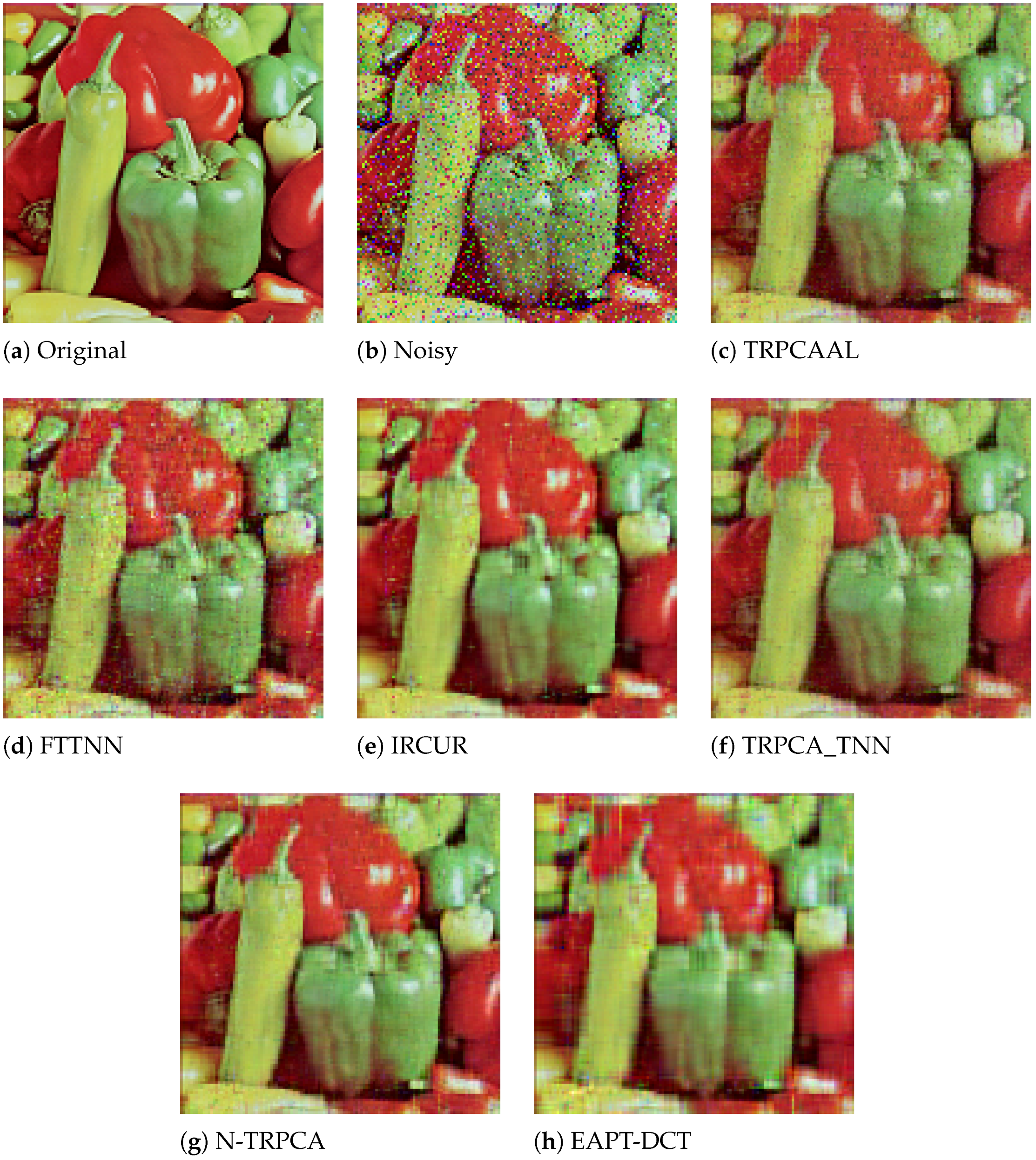
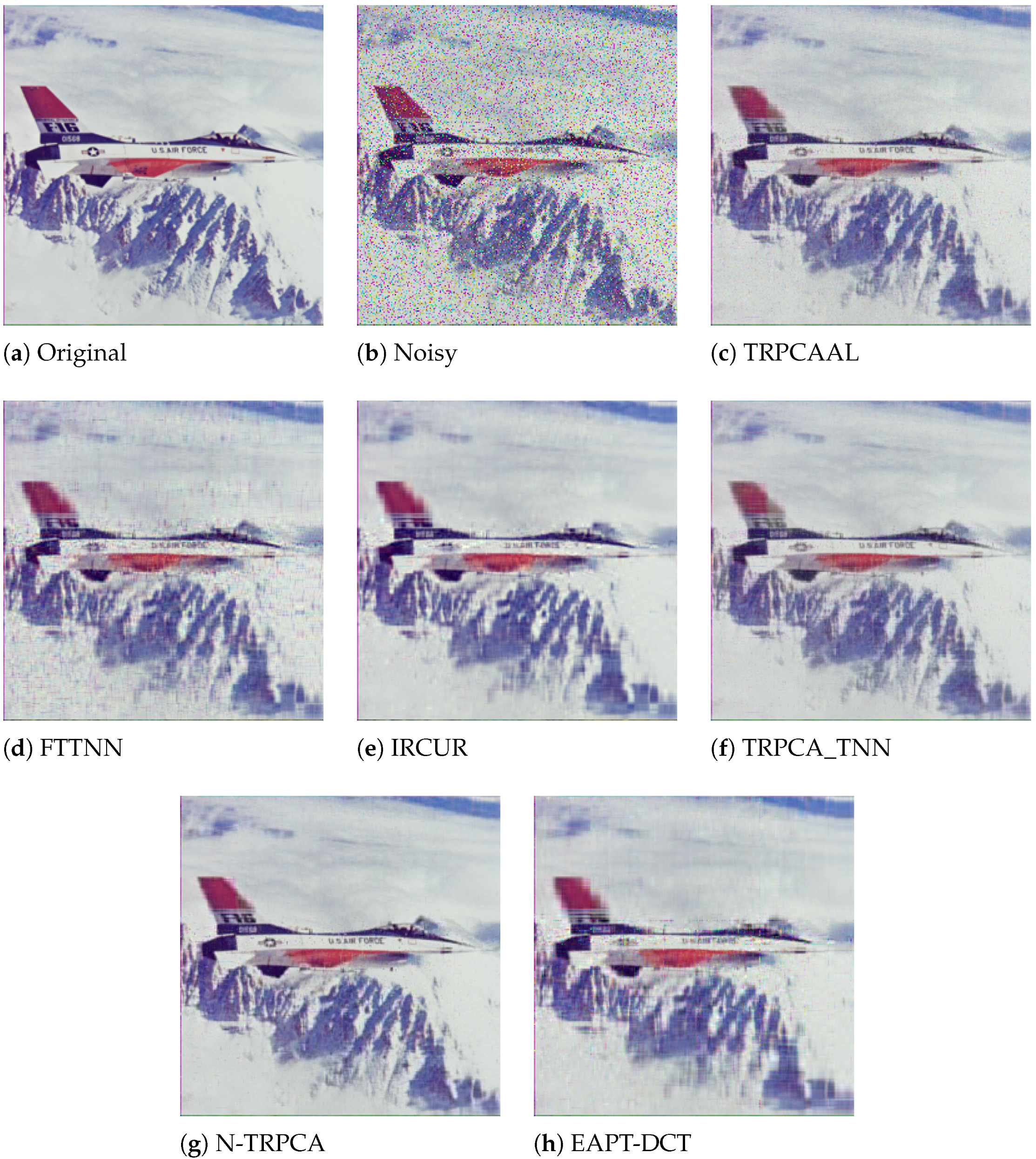
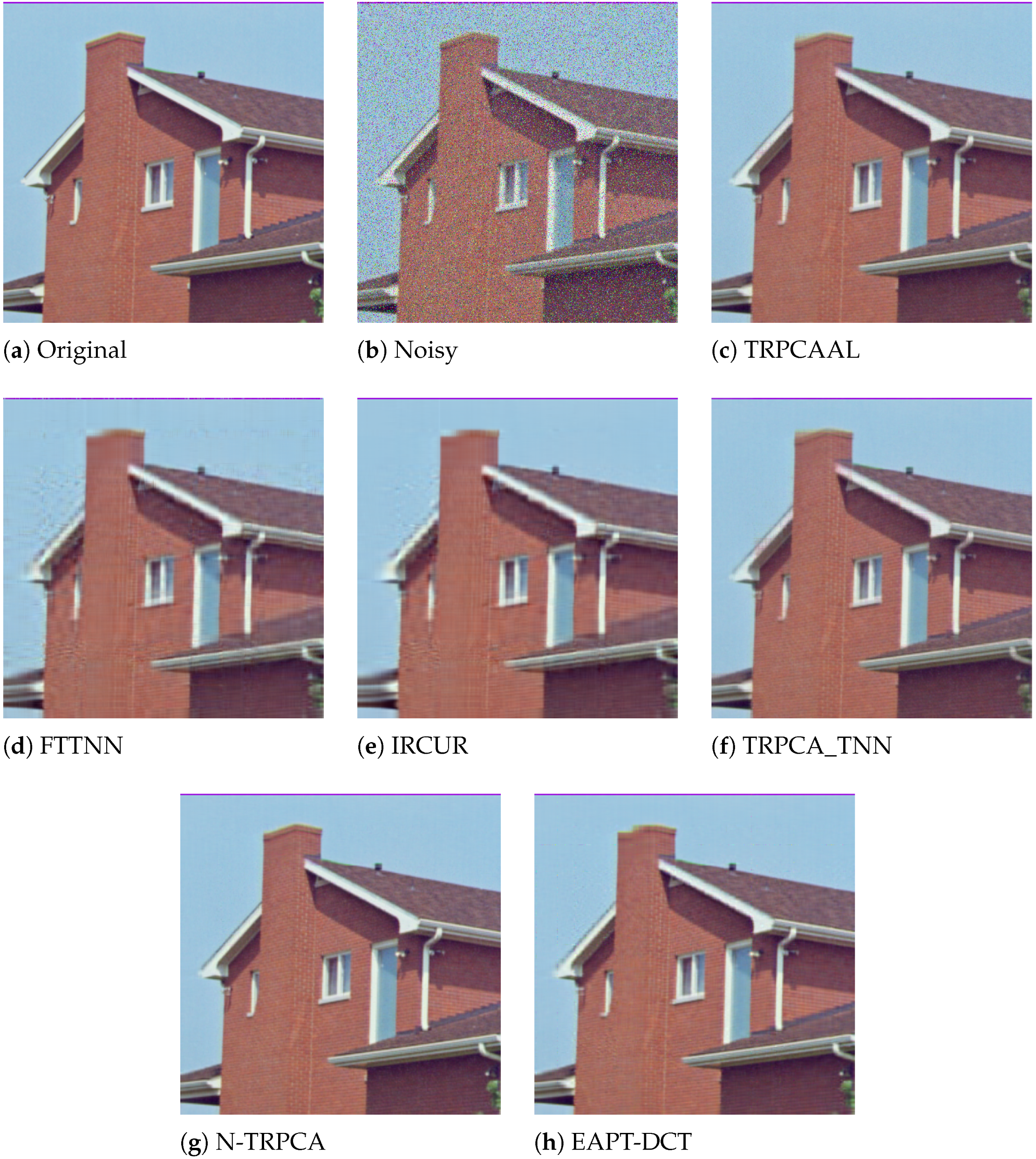
5.1. Color Image Recovery

Color images may contain sparse and impulse noise due to sensor malfunction, external interference, or transmission errors caused by network issues. Such noise significantly degrades the performance of image processing and computer vision algorithms, necessitating the separation of sparse noise from the image as a pre-processing step. One effective solution for recovering color images is to apply TRPCA models, which approximate the clean image as a low-rank tensor under sparse noise corruption. In this section, we compare the performance of various TRPCA algorithms in the context of color image recovery. To evaluate their effectiveness, we use three popular test images: “peppers”, “airplane”, and “house”, shown in Figure 1a, Figure 2a, and Figure 3a, respectively. The image sizes are $128\times 128,256\times 256$, and $512\times 512$. Impulse noise with random magnitudes and positions is added to the test images at different noise levels (10%, 20%, and 40%). Note that the noise level indicates the proportion of image pixels corrupted by impulse noise relative to the total number of pixels. Example images corrupted with 20% noise are shown in Figure 1b, Figure 2b, and Figure 3b.

To compare the performance, we measured the execution time, the number of iterations to converge, and the peak signal-to-noise ratio (PSNR), defined as

$$\mathrm{PSNR}=10{\log }_{10}\left({\displaystyle \frac{{\left|\right|\mathcal{X}\left|\right|}_{\infty }^2}{\frac{1}{n_1{n}_2{n}_3}{\parallel \mathcal{X}-\mathcal{L}\parallel }_F^2}}\right),$$

where $\mathcal{X}$ represents the original image and $\mathcal{L}$ is the low-rank approximated image recovered by the algorithms. The PSNR value quantifies the overall differences between the original and recovered image. For further evaluation of recovery accuracy, we use the feature similarity index (FSIM) [25], which emphasizes structural similarity between the original and recovered image. For all algorithms, we set the stopping criterion $ϵ=1e-4$ and the maximum iteration number as 500. The stopping criterion is defined as

$${\displaystyle \frac{\parallel {\mathcal{L}}_k-{\mathcal{L}}_{k-1}{\parallel }_F}{\parallel {\mathcal{L}}_{k-1}{\parallel }_F}}\le ϵ.$$

The hyperparameters is empirically chosen, for example $r,\lambda$ and $\mu$ for TRPCAAL. Figure 4 illustrates PSNR and execution time as functions of $\mu$ and r using the “airplane” image with 20% random noise. The trends in the plots indicates that the choice of r is more important to the accuracy of TRPCAAL, while its effect on execution time is minimal. This implies that the proposed algorithm maintains computational stability. Throughout the additional experiments, we found that varying $\lambda$ had a negligible impact on performance, so we fixed $\lambda =0.1$. For the other algorithms, we empirically selected the hyperparameters to optimize recovery accuracy.

Table 1. Experimental results for the “peppers” image with 10%, 20%, and 40% noise levels. The top two results in execution time and accuracy are bolded.

Noise		Iterations	Execution Time	PSNR (dB)	FSIM
10%	noisy image	-	-	18.0072	0.8318
	TRPCAAL	9.00	0.0404	25.6008	0.9305
	FTTNN	27.00	0.1343	23.8266	0.8816
	IRCUR	5.95	1.1376	22.9337	0.8581
	TRPCA_TNN	59.45	0.2261	23.5337	0.9051
	N-TRPCA	-	1.1046	25.4216	0.9369
	EATP-DCT	12.30	0.0494	22.6369	0.8710
20%	noisy image	-	-	14.9630	0.7333
	TRPCAAL	11.00	0.0426	22.0561	0.8594
	FTTNN	27.00	0.1376	20.7689	0.8095
	IRCUR	5.95	1.1420	19.8246	0.7855
	TRPCA_TNN	58.75	0.2232	21.9983	0.8615
	N-TRPCA	-	1.3306	23.2304	0.8950
	EATP-DCT	11.70	0.0484	20.5974	0.8285
40%	noisy image	-	-	11.9594	0.6209
	TRPCAAL	12.90	0.0240	17.3287	0.7286
	FTTNN	25.00	0.1144	17.5832	0.7196
	IRCUR	5.85	1.1113	16.5159	0.6955
	TRPCA_TNN	58.55	0.2312	16.9219	0.7254
	N-TRPCA	-	1.1406	18.8762	0.7780
	EATP-DCT	11.45	0.0442	16.0244	0.7030

,

Table 2. Experimental results for the “airplane” image with 10%, 20%, and 40% noise levels. The top two results in execution time and accuracy are bolded.

Noise		Iterations	Execution Time	PSNR (dB)	FSIM
10%	noisy image	-	-	17.4030	0.7873
	TRPCAAL	7.00	0.1922	30.8806	0.9564
	FTTNN	26.00	0.3211	26.5445	0.8668
	IRCUR	5.95	3.2608	26.0213	0.8629
	TRPCA_TNN	58.10	1.0414	28.1301	0.9327
	N-TRPCA	-	5.0506	32.2581	0.9691
	EATP-DCT	19.70	0.3506	26.8569	0.8964
20%	noisy image	-	-	14.3960	0.6763
	TRPCAAL	12.00	0.1444	27.0307	0.9083
	FTTNN	26.00	0.3311	24.6861	0.8249
	IRCUR	5.90	3.2266	23.1291	0.7837
	TRPCA_TNN	58.10	1.0400	26.4528	0.9040
	N-TRPCA	-	5.0613	29.3179	0.9409
	EATP-DCT	19.05	0.3411	23.8989	0.8517
40%	noisy image	-	-	11.4025	0.5574
	TRPCAAL	14.00	0.1090	21.4635	0.7780
	FTTNN	24.00	0.2807	19.4878	0.6968
	IRCUR	5.85	2.3384	17.9545	0.6502
	TRPCA_TNN	57.60	1.0468	20.0816	0.7619
	N-TRPCA	-	5.0344	23.6163	0.8286
	EATP-DCT	14.45	0.2787	15.3644	0.6345

and

Table 3. Experimental results for the “house” image with 10%, 20%, and 40% noise levels. The top two results in execution time and accuracy are bolded.

Noise		Iterations	Execution Time	PSNR (dB)	FSIM
10%	noisy image	-	-	18.6444	0.8690
	TRPCAAL	8.00	0.3435	37.7254	0.9915
	FTTNN	26.00	1.0196	33.9594	0.9725
	IRCUR	6.80	16.1834	33.5131	0.9698
	TRPCA_TNN	58.05	4.3278	35.6128	0.9838
	N-TRPCA	-	19.4259	42.1522	0.9976
	EATP-DCT	24.10	1.4197	35.2786	0.9740
20%	noisy image	-	-	15.6322	0.7935
	TRPCAAL	13.15	0.5223	34.3571	0.9830
	FTTNN	25.00	0.8425	29.5879	0.9186
	IRCUR	5.90	10.6101	28.1123	0.9047
	TRPCA_TNN	57.25	4.2798	33.0207	0.9730
	N-TRPCA	-	19.4864	38.8358	0.9940
	EATP-DCT	27.35	1.5598	33.9489	0.9716
40%	noisy image	-	-	12.6272	0.6913
	TRPCAAL	17.10	0.5034	27.0085	0.9195
	FTTNN	24.00	0.7682	23.6106	0.8241
	IRCUR	19.20	18.1779	24.3123	0.8327
	TRPCA_TNN	56.60	4.3993	24.7224	0.9139
	N-TRPCA	-	20.2492	31.5374	0.9640
	EATP-DCT	44.80	2.3762	20.3844	0.8389

present the experimental results for all algorithms. In the tables, the top two performing results in each category are highlighted for easier comparison. Additionally, example outputs with 20% random noise are shown in Figure 1, Figure 2 and Figure 3. From the results, we observe that N-TRPCA consistently achieves the highest accuracy in terms of PSNR and FSIM across most scenarios in the color image recovery application. However, as evident from the data, its execution time is significantly longer than that of the other algorithms. Apart from N-TRPCA, TRPCAAL generally ranks as the second most accurate algorithm, except in the cases of the “peppers” image with 20% and 40% noise, where FTTNN and TRPCA_TNN show slightly better accuracy. Nevertheless, even in these cases, the performance of TRPCAAL is only marginally lower. What makes TRPCAAL stand out is its execution time—it is the fastest across all test cases. Notably, TRPCAAL’s computational efficiency becomes increasingly apparent as image size increases. For example, when recovering a $128\times 128$ image, TRPCAAL is approximately 33 times faster than N-TRPCA, the slowest among the tested algorithms. This gap widens to 43 times for a $512\times 512$ image. Compared to the other algorithms known for their faster execution, TRPCAAL still outperforms them in execution time.

An additional experiment was conducted using the “airplane” image with impulse noises containing extremely large magnitudes—50 times greater than the maximum pixel brightness—to simulate gross corruptions or outlier entries in sparse locations. All hyperparameters for algorithms were selected empirically.

Table 4. Experimental results for the “airplane” image with 10%, 20%, and 40% noise levels. The top two results in execution time and accuracy are bolded.

Noise		Iterations	Execution Time	PSNR (dB)	FSIM
10%	noisy image	-	-	14.5079	0.0965
	TRPCAAL	65.95	0.6039	29.6132	0.9305
	FTTNN	20.00	0.2796	4.7797	0.0898
	IRCUR	22.25	10.0694	15.5529	0.6053
	TRPCA_TNN	63.00	1.2621	12.9168	0.6503
	N-TRPCA	-	6.2646	32.3481	0.9704
	EATP-DCT	24.25	0.3680	12.9846	0.3860
20%	noisy image	-	-	11.5019	0.0263
	TRPCAAL	67.45	0.6158	27.1214	0.9012
	FTTNN	20.00	0.2926	4.5666	0.0615
	IRCUR	21.35	9.6075	15.0562	0.5743
	TRPCA_TNN	62.15	1.2326	10.6987	0.5592
	N-TRPCA	-	6.2572	29.5371	0.9449
	EATP-DCT	23.15	0.3483	8.9972	0.1999
40%	noisy image	-	-	8.4811	0.0135
	TRPCAAL	87.85	0.6828	21.9168	0.7935
	FTTNN	20.00	0.2797	4.5093	0.0427
	IRCUR	20.20	9.1873	13.8373	0.4780
	TRPCA_TNN	62.00	1.2249	8.1658	0.4618
	N-TRPCA	-	6.2689	24.1166	0.8463
	EATP-DCT	24.00	0.3597	4.6647	0.0194

presents the experimental results. Similar to the experiments with random pixel noise, Algorithm 1 and N-TRPCA achieved the highest accuracy, as indicated by high PNSR and FSIM values. However, aside from these two algorithms, the others failed to produce meaningful outputs in the presence of outliers, even though some of them exhibited a faster execution time. Overall, the proposed algorithm achieves reasonably high recovery accuracy while offering the fastest execution speed, making it a highly appealing solution for large-scale color image recovery problems.

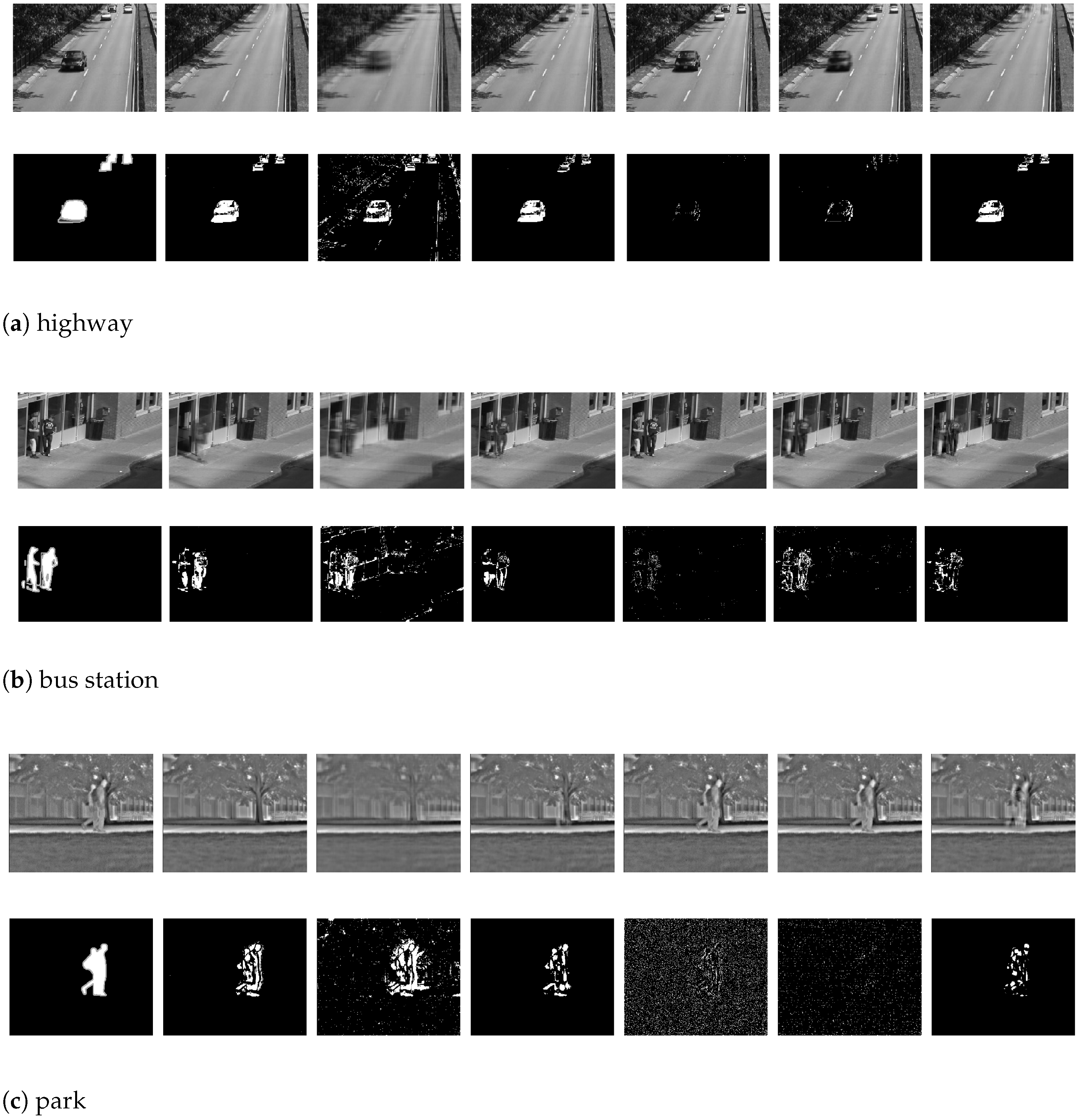
5.2. Background Subtraction

Another popular application of TRPCA is background subtraction. Since the video sequences can be modeled as a combination of a static background (low-rank component) and moving objects (sparse component), the background subtraction problem can be effectively addressed using TRPCA algorithms [26]. To evaluate the performance of the algorithms, three video sequences are used, which include the “highway”, “Bus station”, and “park”. We extract 300 frames from the video sequences with frame sizes of $240\times 320$, $240\times 360$, and $288\times 352$, respectively. To assess the accuracy of background subtraction, we compute precision, recall, and F-score based on the foreground detection results and corresponding ground-truth data. As in the color image recovery experiment in Section 5.1, we set the stopping criterion $ϵ=1.0e-4$ for all algorithms. The hyperparameters for each algorithms are chosen empirically to achieve the highest possible F-score value.

Table 5. Experimental results for the “highway” video sequence. The top two results in terms of execution time and F-score are bolded for comparison.

Noise		Iterations	Execution Time	Precision	Recall	F-Score
	TRPCAAL	4	3.7391	0.5295	0.5672	0.5407
	FTTNN	25	32.6119	0.4749	0.1468	0.2041
	IRCUR	24	513.9714	0.4855	0.5898	0.5269
	TRPCA_TNN	43	82.7404	0.0244	0.4375	0.0456
	N-TRPCA	-	249.2075	0.0954	0.3753	0.1474
	EATP-DCT	25	32.9607	0.4377	0.5587	0.4826

,

Table 6. Experimental results for the “bus station” video sequence. The top two results in terms of execution time and F-score are bolded for comparison.

Noise		Iterations	Execution Time	Precision	Recall	F-Score
	TRPCAAL	4	4.2106	0.3719	0.5477	0.4356
	FTTNN	25	36.8798	0.3322	0.1521	0.2047
	IRCUR	24	585.0544	0.1704	0.6491	0.2565
	TRPCA_TNN	43	93.0426	0.1195	0.1549	0.1310
	N-TRPCA	-	287.7277	0.7393	0.0243	0.0470
	EATP-DCT	26	38.5858	0.1635	0.5586	0.2455

and

Table 7. Experimental results for the “park” video sequence. The top two results in terms of execution time and F-score are bolded for comparison.

Noise		Iterations	Execution Time	Precision	Recall	F-Score
	TRPCAAL	4	4.9572	0.2727	0.4436	0.3294
	FTTNN	24	35.0960	0.3105	0.0738	0.1157
	IRCUR	23	658.9767	0.2541	0.5875	0.3475
	TRPCA_TNN	40	112.5505	0.6425	0.0201	0.0387
	N-TRPCA	-	346.1222	0.0583	0.0329	0.0396
	EATP-DCT	26	45.2597	0.1281	0.5621	0.2040

summarize the performance comparison of the algorithms. Note that the precision, recall, and F-score values presented in Table 5, Table 6 and Table 7 are averaged over all video frames. Figure 5a–c illustrate example frames from the video sequences, along with their ground-truth background subtraction results and the outputs from each algorithm. From the results, TRPCAAL consistently achieved the fastest execution time while maintaining competitive or the best F-score values across all video sequences, demonstrating strong overall performance in both speed and accuracy. Unlike the experimental results in color image recovery, N-TRPCA produced unsatisfactory results in both accuracy and execution time. While IRCUR achieved slightly higher F-score values in some cases, it suffered from extremely high execution times, making it impractical for real-time or large-sized video sequences. Therefore, TRPCAAL emerges as the most attractive choice, providing accurate results with minimal computational cost in background subtraction.

6. Conclusions

TRPCA is widely used in various applications due to its ability to separate a low-rank approximated tensor and sparse noise from the data. However, because the problem involves manipulating large-scale and complexly structured data, TRPCA typically requires substantial computational resources. To address this limitation, we propose a novel TRPCA computation approach by relaxing the tensor nuclear norm minimization into an optimization problem involving the sum of Frobenius norms of factor tensors. Since the low-rank approximated tensor can be represented using truncated factor tensors, we alternatingly update these factor tensors to efficiently compute the low-rank approximation with reduced computational cost. Experimental results show that the proposed method significantly outperforms other state-of-the-art TRPCA algorithms in terms of execution time while maintaining highly accurate recovery performance in practical applications such as color image recovery and background subtraction.

References

1. Candès, E.J.; Li, X.; Ma, Y.; Wright, J. Robust Principal Component Analysis? J. ACM 2011, 58, 1–37. [Google Scholar] [CrossRef]
2. Bouwmans, T.; Javed, S.; Zhang, H.; Lin, Z.; Otazo, R. On the Applications of Robust PCA in image and Video Processing. Proc. IEEE 2018, 160, 1427–1457. [Google Scholar] [CrossRef]
3. Cao, W.; Wang, Y.; Sun, J.; Meng, D.; Yan, C.; Cichocki, A.; Xu, Z. Total Variation Regularized Tensor RPCA for Background Subtraction from Compressive Measurement. IEEE Trans. Image Proc. 2016, 25, 4075–4090. [Google Scholar] [CrossRef] [PubMed]
4. Hu, Y.; Liu, J.; Gao, Y.; Shang, J. DSTPCA: Double-Sparse Constrained Tensor Principal Component Analysis Method for Feature Selection. IEEE/ACM Trans. Comput. Biol. Bioinform. 2021, 18, 1481–1491. [Google Scholar] [CrossRef]
5. Markowitz, S.; Snyder, C.; Eldar, Y.C.; Do, M.N. Mutilmodal unrolled robust RPCA for background foreground separation. IEEE Trans. Image Proc. 2022, 31, 3553–3564. [Google Scholar] [CrossRef]
6. Zhong, G.; Pun, C.M. RPCA-induced self-representation for subspace clustering. Neurocomputing 2021, 437, 249–260. [Google Scholar] [CrossRef]
7. Cai, J.F.; Candès, E.J.; Shen, Z. A singular value thresholding algorithm for matrix completion. SIAM J. Optim. 2010, 20, 1956–1982. [Google Scholar] [CrossRef]
8. Kolda, T.G.; Bader, B.W. Tensor decomposition and applications. SIAM Rev. 2009, 51, 455–500. [Google Scholar] [CrossRef]
9. Hillar, J.C.; Lim, L.H. Most tensor problems are NP-Hard. J. ACM 2013, 60, 1–39. [Google Scholar] [CrossRef]
10. Liu, J.; Musialski, P.; Wonka, P.; Ye, J. Tensor completion for estimating missing values in visual data. IEEE Trans. Pattern Anal. Mach. Intell. 2013, 35, 208–220. [Google Scholar] [CrossRef]
11. Kilmer, M.E.; Martin, C.D. Factorization strategies for third-order tensors. Linear Algebra Appl. 2011, 435, 641–658. [Google Scholar] [CrossRef]
12. Kilmer, M.E.; Horesh, L.; Avron, H.; Newman, E. Tensor-tensor algebra for optimal representation and compression of multiway data. Proc. Natl. Acad. Sci. USA 2021, 118, e205851118. [Google Scholar] [CrossRef]
13. Lu, C.; Feng, J.; Chen, Y.; Liu, W.; Lin, Z.; Yan, S. Tensor Robust Principal Component Analysis with a New Tensor Nuclear Norm. IEEE Trans. Pattern Anal. Mach. Intell. 2020, 42, 925–938. [Google Scholar] [CrossRef]
14. Zhang, Z.; Ely, G.; Aeron, S.; Hao, N.; Kilmer, M.E. Novel methods for multilinear data completion and de-noising based on tensor-SVD. IEEE Conf. Comput. Vis. Pattern Recognit. 2014, 3842–3849. [Google Scholar] [CrossRef]
15. Gao, Q.; Zhang, P.; Xia, W.; Xie, D.; Gao, X.; Tao, D. Enhanced Tensor RPCA and its Application. IEEE Trans. Pattern Anal. Machine Intell. 2021, 43, 2133–2140. [Google Scholar] [CrossRef] [PubMed]
16. Dong, H.; Tong, T.; Ma, C.; Chi, Y. Fast and provable tensor robust principal component analysis via scaled gradient descent. Inform. Inference J. IMA 2023, 12, iaad019. [Google Scholar] [CrossRef]
17. Qui, H.; Wang, Y.; Tang, S.; Meng, D.; Yao, Q. Fast and Provable Nonconvex Tensor RPCA. In Proceedings of the 39th International Conference on Machine Learning, Baltimore, MI, USA, 17–23 July 2022. [Google Scholar]
18. Geng, X.; Guo, Q.; Hui, S.; Yang, M.; Zhang, C. Tensor robust PCA with nonconvex and nonlocal regularization. Comput. Vision Image Understand 2024, 243, 104007. [Google Scholar] [CrossRef]
19. Qui, Y.; Zhou, G.; Huang, Z.; Zhao, Q.; Xie, S. Efficient Tensor Robust PCA Under Hybrid Model of Tucker and Tensor Train. IEEE Sig. Proc. Lett. 2022, 29, 627–631. [Google Scholar]
20. Cai, H.; Chao, Z.; Huang, L.; Needell, D. Fast Robust Tensor Principal Component Analysis via Fiber CUR Decomposition. IEEE/CVF Int. Conf. Comput. Vision Work. 2021, 189–197. [Google Scholar] [CrossRef]
21. Salut, M.M.; Anderson, D.V. Online Tensor Robust Principal Component Analysis. IEEE Access 2022, 10, 69354–69363. [Google Scholar] [CrossRef]
22. Hastie, T.; Mazumder, R.; Lee, J.D.; Zadeh, R. Matrix Completion and Low-Rank SVD via Fast Alternating Least Squares. J. Machin. Learn. Res. 2015, 16, 3367–3402. [Google Scholar]
23. Mazumder, R.; Hastie, T.; Tibshirani, R. Spectral Regularization Algorithms for Learning Large Incomplete Matrices. J. Machine Learn. Res. 2010, 11, 2287–2322. [Google Scholar]
24. Tibshirani, R. Regression shrinkage and selection via the lasso: A retrospective. J. R. Stat. Soc. 2011, 73, 273–282. [Google Scholar] [CrossRef]
25. Zhang, H.; Gong, C.; Qian, J.; Zhang, B.; Xu, C.; Yang, J. Efficient recovery of low-rank via double nonconvex nonsmooth rank minimization. IEEE Trans. Neural Net. Learn. Syst. 2019, 30, 2916–2925. [Google Scholar] [CrossRef]
26. Bouwmans, T.; Zahzah, E.H. Robust PCA via Principal Component Pursuit: A review for a comparative evaluation in video surveillance. Comput. Vision Image Understand 2014, 122, 22–34. [Google Scholar] [CrossRef]
Figure 1. Test images used in color image recovery when the “peppers” image with 20% random noise is used.
Applsci 15 08114 g001
Figure 2. Test images used in color image recovery when the “airplane” image with 20% random noise is used.
Applsci 15 08114 g002
Figure 3. Test images used in color image recovery when the “house” image with 20% random noise is used.
Applsci 15 08114 g003
Figure 4. Empirical hyperparameter selection based on the variation in μ and r. Note that the “airplane” image with 20% random noise is used.
Applsci 15 08114 g004
Figure 5. Background subtraction results from video sequences. From left to right, original frame and output from TRPCAAL, FTTNN, IRCUR, TRPCA_TNN, N-TRPCA, and EAPT-DCT, respectively.
Applsci 15 08114 g005