The Estimation of the Remaining Useful Life of Ceramic Plates Used in Iron Ore Filtration Through a Reliability Model and Machine Learning Methods Applied to Industrial Process Variables of a Pims

Abstract

The intensive use of various sensors in industrial machines has the potential to indicate the real-time health status of critical equipment. This is achieved through the connectivity of their automation systems (PIMS and MES), enabling the optimization of the preventive maintenance interval, a reduction in corrective maintenance and safety-related failures, an increase in productivity and reliability and a reduction in maintenance costs. Through the use of the CRISP-DM data analysis methodology, the fault logs of ceramic plates applied in an iron ore filtration process are coupled with sensor readings of the process variables over the time of operation to create exponential survival models via two techniques: a multiple linear regression model with averaged data and a random forest regression machine learning model with individual instant data. The instantaneous reliability of ceramic plates is then used in the online prediction of the remaining useful life of the components. The model obtained from the instantaneous reading of 12 sensors led to the estimation of the remaining useful life for ceramic plates with up to 5600 h of use, allowing the adoption of a strategy of replacing these components by condition instead of replacing them by a fixed time, leading to increased process reliability and improved stock planning. The linear regression model for reliability prediction had an R² of 78.32%, whereas the random forest regression model had an R² of 63.7%. The final model for predicting the remaining useful life had an R² of 99.6%.

1. Introduction

Industry 4.0 concepts lead to the generation of large amounts of data, many of which are available in real time to end users; however, these data are often not effectively used to their maximum potential for prediction, diagnosis and prescription for decision-making related to the production process and maintenance of industrial equipment.

The use of process variables and sensors can assist in the early diagnosis of common failure modes that negatively impact product quality in industries and the availability of critical equipment. Digitalization concepts, the application of advanced statistical concepts and data science can enable the early diagnosis of chronic failure modes, reduce machine downtime, reduce risk and improve resource allocation. Well-established data analysis methodologies such as CRISP-DM establish a framework for analyzing complex business problems in a structured way.

Equipment and component failure data can be analyzed in statistical reliability analysis models to estimate the probability of failure over time, and sensor data can indicate different failure states, enabling the early assessment of a component’s end of life through sensor reading pattern classification. Areas of knowledge seeing growing interest, such as online predictive maintenance and RUL—remaining useful life—aim to establish the relationship between sensor readings and the remaining useful life of machines and components. Previous studies employed similar methodologies in the analysis of sensors to identify failures in bearings, gears, wind turbines, marine turbines, aeronautical engines, filters, electric batteries and other equipment in the early prediction of failures through the identification of patterns and anomalies in equipment process variables in the time or frequency domain, but most of these studies considered the use of sensors dedicated specifically to this purpose.

The objective of this work is to present a methodology that allows the processing of large volumes of data, enabling the prediction of the reliability and remaining useful life of industrial systems and components from data that are already collected and processed in automation systems such as PIMSs—Plant Information Management Systems—and the MES—Manufacturing Enterprise System—without the need for additional sensors. Sensor readings used for simple problem identification in industrial automation in high–low alarms and high–high and low–low safety protocols can be used in analytical models to identify more complex process anomalies earlier.

This work presents a case study for ceramic plates from vacuum filters in an iron ore slurry filtration industry where operational process variables and failure data were used to determine a model for their remaining useful life. Ceramic plates represent one of the highest costs of an industrial filtration plant, corresponding to more than 40% of its annual operational budget, and they also have a high impact on filter productivity and iron ore moisture content. These characteristics lead to ceramic plate components that must be replaced as minimally as possible, keeping their performance reliably within process requirements. Replacing them earlier than required causes unnecessary costs, whereas late replacement can cause a loss of process control.

2. Theoretical Framework

2.1. RUL: Reliability and Predictive Maintenance

Kundu, P. et al. [1] stated that easier access to data resulting from the technical advances brought about by Industry 4.0 increased the use of tools to predict failures and reduce their effects through failure prognostic information. Most studies focus on estimating the remaining useful life (RUL).

There are three possible maintenance strategies [2]. In reactive maintenance, a machine or component is used until its failure. In preventive maintenance, failures are avoided through maintenance carried out at predefined time intervals. In predictive maintenance, the time to failure of a machine is estimated, which helps in maintenance scheduling and reduces the probability of unexpected failures. Figure 1 presents each maintenance strategy in a graph of machine health as a function of time and the effect of performing maintenance at different points in time.

According to Lei, Y. et al. [3] and Qin, A. et al. [4], the prognosis of machinery is one of the main functions of condition-based maintenance to predict its remaining useful life. This research area employs techniques that provide early warnings of failures, which are important in managing the health of systems and machines. Wang, Q. et al. [5] defined the remaining useful life of a piece of equipment or component as the time until it reaches the end of its useful life.

Liu, G. et al. [6] established that the term is widely used in analyses in industries and presented a study estimating the remaining useful life of power generation machines in the nuclear industry. Qin, A et al. [4] presented a general application for rotating machinery.

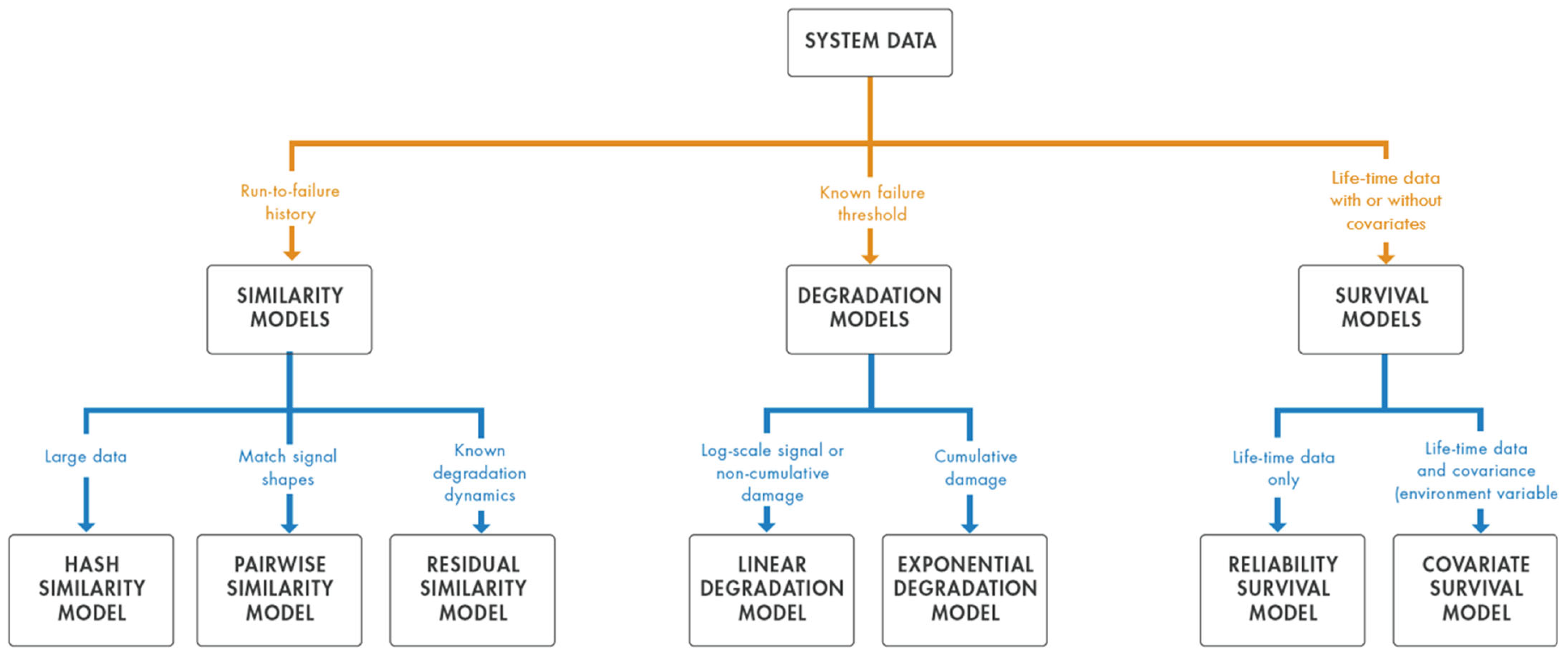
There are three ways to estimate the remaining useful life of equipment [2], as presented in Figure 2.

One of these forms, reliability analysis, involves a probabilistic function whose main distributions are the normal, exponential, lognormal and Weibull distributions [7,8,9].

Many authors [7,8,9,10,11,12] have presented applications and developments of reliability studies using the exponential model. These studies highlight the low complexity of the model as the main advantage, even though the lack of memory is an important limitation that must be considered.

Montgomery, D. [13] established the probability density function of a random variable X with an exponential distribution, its mean and its variance as follows:

$$f(x)=\lambda e^{-\lambda x} for 0 \le x<\infty$$

$$\mu =E(X)={\displaystyle \frac{1}{\lambda }}$$

$${\sigma }^{2 }=V(X)={\displaystyle \frac{1}{{\lambda }^2}}$$

2.2. CRISP-DM: Framework for Data Analysis

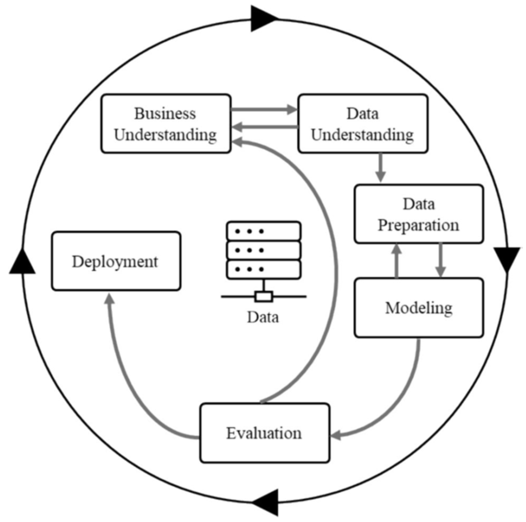
According to Bokrantz, J. et al. [14], CRISP-DM has been successfully applied because of its practical orientation, agility and flexibility, and it is currently known as the standard for application in data mining projects. Doede, N. et al. [15] and Wiemer, H. et al. [16] presented the meaning of the acronym, this being Cross-Industry Standard Process for Data Mining. Figure 3 presents a schematic diagram of the steps applied in this methodology.

2.3. Machine Learning: Prediction via Linear Regression

According to Gayathri, R., et al. [17], linear regression is a statistical method used to analyze the effect of one or more input variables, with one output variable, being one of the most popular machine learning algorithms. In simple linear regression, there is only one independent variable x and a dependent variable y, whereas in multiple linear regression, there are two or more independent variables.

Montgomery, D. [13] established that although the relationship between variables is well represented by a linear regression, the observed values contain an error, and the expression for an adjusted linear regression is

$$y=\widehat{b_0}+\widehat{b_1}{x}_1+{\widehat{b_2}{x}_2+\cdots +\widehat{b_n}{x}_n+\in }_i$$

where $\widehat{b_0 }, \widehat{b_1}, \cdots$ are the estimates obtained via the least squares method and where ${\in }_i=y_i-\widehat{y_i}$ is the residual, which describes the error in the model fitted value for the ith observation y.

2.4. Machine Learning: Random Forest Regression Algorithm

According to Tayade, A. et al. [18], the random forest model stands out among machine learning models for predictive analytics applications and is useful in approaching databases in tabular forms with numerical and categorical variables. Kundu, P. et al. [1] stated that there are advantages of the method in that it is nonparametric, easy to understand and quick to adjust, even in large problems, in addition to it not requiring deep statistical knowledge. It is an additive model that makes predictions by grouping decisions from a sequence of base models, and unlike linear models, it can interpret nonlinear behaviors between variables. The model can be written according to the following equation:

$$g(x)=f_0(x)+f_1(x)+f_2(x)+\cdots$$

where g is the last model, given by adding the $f_i$ base models. The basic models are built by partitioning the data, turning it into independent decision trees.

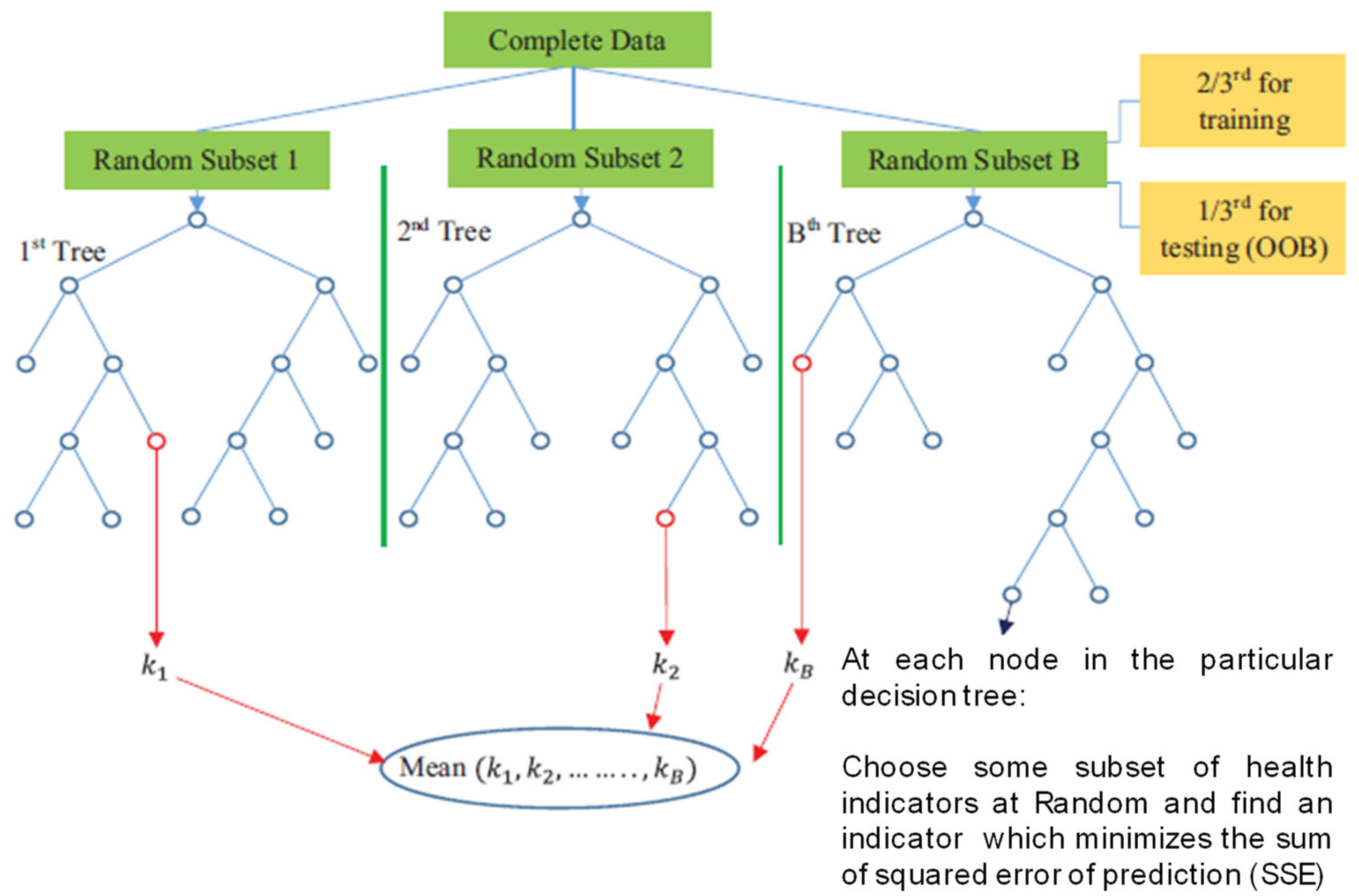
Kundu, P. et al. [1] explained that the approach employs bootstrap sampling, which consists of sampling with replacement, to reduce the variance in predictors through predictions made by multiple models of decision trees trained with subsamples of the same database. The schematic diagram presented in Figure 4 indicates with red arrows the bootstrap sampling process, where the prediction is obtained by calculating the average for every corresponding split for B trees. The diagram also indicates that for each node, two thirds of the database is used for model training, and one third is used for testing, known as the out-of-bag sample (OOB).

The authors [1] summarize the method as follows:

• For nodes b = 1 through B:

• A size n × p bootstrap sample is used for size N × p training data, where N is the number of observations, p is the number of variables and n is a sample of N.
• A decision tree $T_{b }$ is created based on the sampled data via the minimization criterion of $\mathrm{S}\mathrm{S}\mathrm{E}={\sum }_{i=1}^n{(y_i-{\overline{y}}_R)}^2$, where $y_i$ represents the observed values and ${\overline{y}}_R$ represents the mean fitted values. The sampled data is divided recursively according to the following steps:
  • For each node, select m variables (out of the total p variables) and split points;
  • Among the variables, select the best variable and its best division points;
  • Split each parent node between two child nodes.

2.

B decision trees are developed via the procedure applied in step 1, as shown in ${\left\{T_b\right\}}_1^B$.

3.

For a given x, the prediction will be the average of the predictions made by the individual decision trees B.

3. Methodological Procedures

The methodology CRISP-DM, combined with the remaining useful life prediction methodology summarized in Figure 5, is applied in this study. The steps of the CRISP-DM method can be related to the steps for the analysis of predictive maintenance and remaining useful life, with the main advantage of the addition of phases aimed at understanding the business and understanding the data.

An overview of the methodology adopted is presented in Figure 5.

Table 1. Description of the steps of the methodology used.

Stage	Description
Business Understanding	Ceramic plates are the main components of a ceramic filter and correspond to approximately 40% of the operating cost of an industrial filtration plant, in addition to having a direct effect on the production capacity and quality of the final product (moisture content). These are the reasons to optimize the useful life of these components, accurately identifying the optimal time to carry out plate set renewals.
Data Acquisition and Data Understanding	Based on the business understanding phase and facility’s database, a selection of 12 sensors is made. According to process specialists, these variables can influence or be influenced by the change in the performance of ceramic plates, and this, alongside reliability models obtained by the failure and replacement data, can be combined to predict the remaining useful life of these components. The sensor reading data are obtained from the PIMS—Plant Information Management System (Osisoft AVEVA PI Vision/PI Datalink ®, ver. 2023 SP1)—and the ceramic plate failure and replacement data are exported from the MES—Manufacturing Enterprise System (Osisoft AVEVA Production Management ®, ver. 2020 U1).
Data Preparation	After identifying the main process variables and obtaining the failure data records, they undergo treatment to remove outliers and missing data. In addition, different data sources are combined into one, making it possible to relate the useful life to the process variables. To prepare the data, electronic spreadsheets in Microsoft Excel® (MS Office 365 version) are used.
Identification of Health Condition Indicators	In this stage, statistical descriptive analyses are carried out to achieve a correct and broad understanding of data that characterizes normal operation, and to determine which are the best indicators for anomalies in these readings over time. With a condition indicator, a time trigger is established in which the reliability of the plate sets reaches 70%. Statistical analysis and modeling are performed using Minitab® software (version 19).
Modeling	Modeling consists of identifying the best models of survival/the reliability of failure and plate replacement data and identifying the best machine learning models that may be able to use sensor readings as predictors of reliability and, ultimately, the remaining useful life of these components. Model creation uses only a fraction of the partitioned data, called the training set.
	In the evaluation of the models, the main statistical metrics are used to evaluate the significance and predictive capacity. In this step, partitioned validation data is used as input into the model for evaluation.
Model Deployment and Integration	After being tested and validated, the model can be released in a production environment in software/systems, being fed back whenever new data becomes available.

presents the specific tasks developed in each stage in the analysis of the prediction of the remaining useful life of ceramic plates.

Case Study: Ceramic Plates in Vacuum Filters

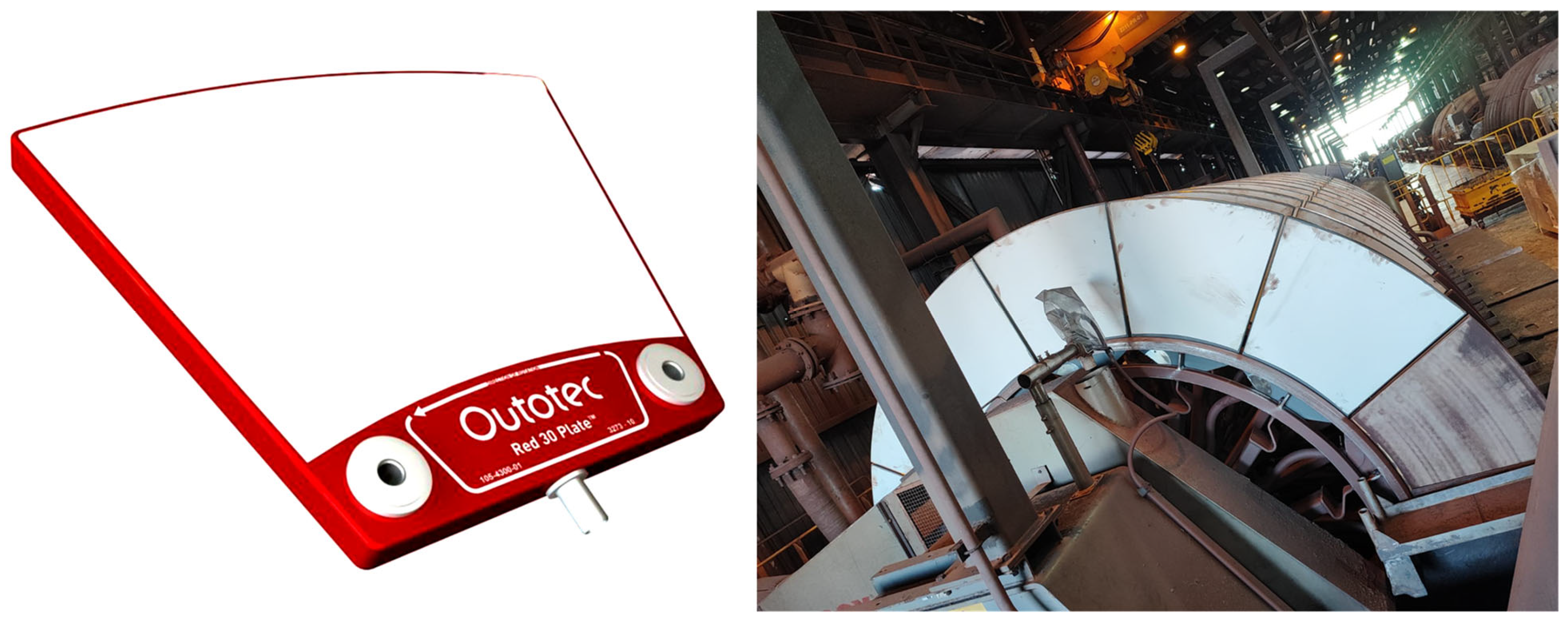
As a case study, an industrial iron ore filtration facility located in Brazil with 14 ceramic filters was analyzed. Figure 6 shows a picture of a new ceramic plate and a ceramic filter undergoing periodic replacement of the entire 180-plate set.

Ceramic plate failure data and ceramic filter sensor reading data were collected to predict the remaining useful life through an analysis of the influence of reliability and process variables on component performance over time.

The Larox^®CC-144, (Lappeenranta, Finland) ceramic filters use 180 ceramic plates with 2 μm pores. Note: Larox is now part of Metso: Outotec company (Espoo, Finland).

The ceramic plates have a manufacturer-specified useful life of 2–3 years of continuous operation; however, several failure modes can affect this lifespan, in which the component is able to maintain its expected performance. The performance and operational acceptability of a filter with a set of plates are controlled through the routine analysis of its operating parameters, production capacity and product quality; thus, the entire set of plates of a ceramic filter is renewed at time intervals that may vary. However, during the period of operation between complete renewals of plate sets, failures may occur, and corrective replacements may be employed.

The main failure modes are indicated in Figure 7. These are the failure modes in which corrective replacements of ceramic plates occur. The figure shows, from left to right, a cracked plate, a broken plate and leakage near the fasteners.

The framework based on the methodologies CRISP-DM and RUL, presented in Figure 5, was applied, and a description of each step is summarized in Table 1.

4. Results and Discussion

4.1. Descriptive Analysis

The database of 12 variables of sensor readings in hourly average values was obtained for the period between January 2021 and June 2024, in addition to failures and corrective replacement records of ceramic plates and complete sets of renewal data.

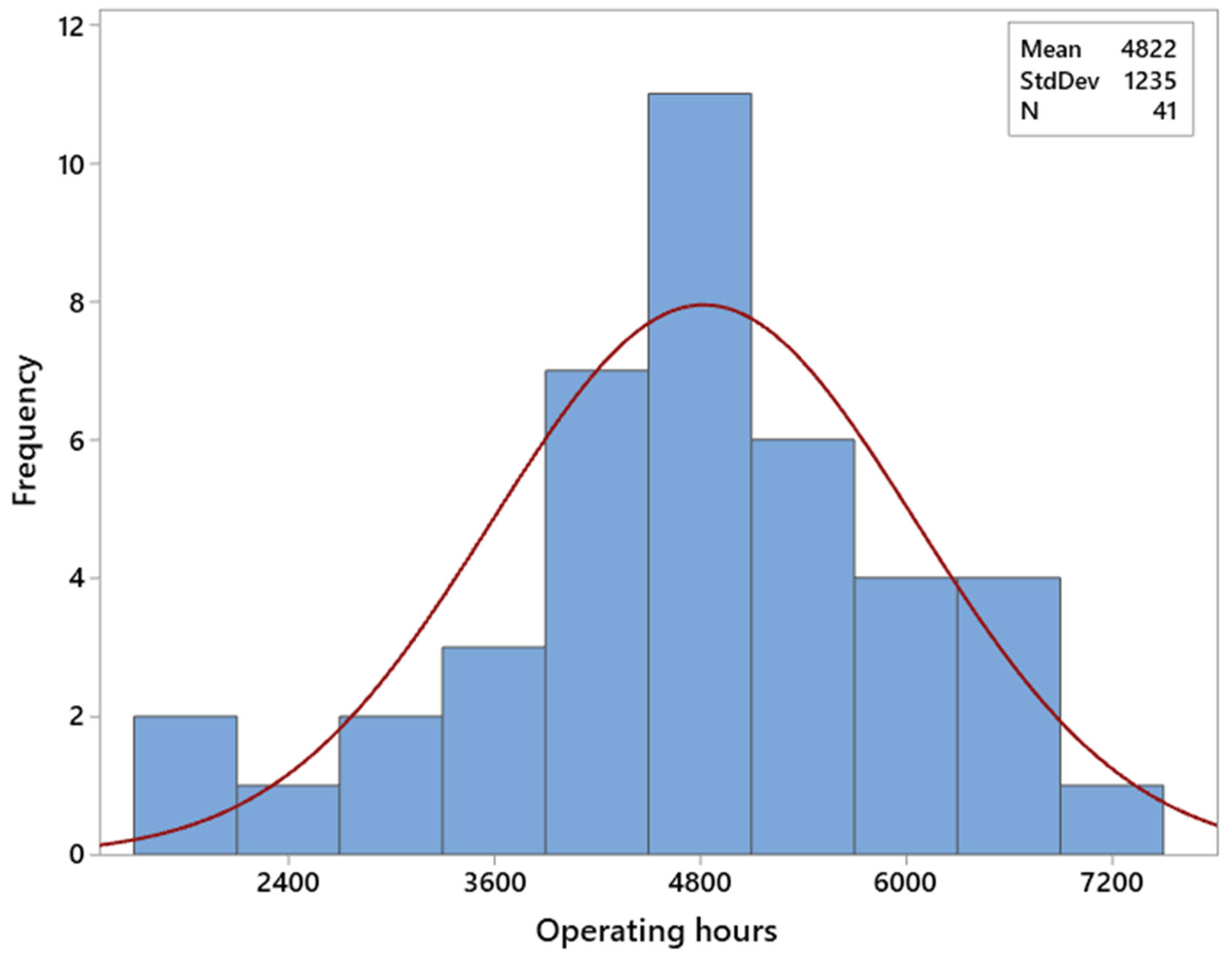
A summary of the distribution of the data analyzed is presented in

Table 2. Distribution of data by period of hours operated.

Hours Operated	Data Operation	Failures
0–1000	29,119	120
1000–2000	29,068	226
2000–3000	27,761	504
3000–4000	25,219	644
4000–5000	18,058	457
5000–6000	4549	97
6000–7000	288	6
Total	134,062	2054

and Figure 8.

4.2. Reliability Model

Using the maximum likelihood estimation method, an exponential distribution is modeled considering both ceramic plate failure data and their preventive substitutions (right-censored data). In Figure 9, a graphical summary of the model is presented, as well as its main parameters and statistics.

Failure data records considered 2795 ceramic plate failures and 7731 right-censored replacements. In the left graph, the survival function represents the probability of survival over the usage of ceramic plates. In the middle graph, an exponential Q-Q plot is presented as a qualitative assessment of how well data can be represented by the exponential distribution. On the right, a box presents a summary of the main statistics of the model. Based on failure and replacement records, ceramic plates have a survival probability of 90% at 1388 operating hours, 80% at 2940 operating hours, 70% at 4700 operating hours and 60% at 12,074 operating hours. As Figure 8 shows, complete ceramic plate renewal occurs on average at 4822 operating hours, and a set never operated longer than 7285 h.

4.3. Linear Regression Model for Reliability Prediction

A linear regression model was adjusted considering all 12 process variables obtained. To determine the best set of predictors in the model,

Table 3. Predictor correlation matrix.

	U129_IIT	U129	U009_IIT	PT325	PT225	PT125	PT101	KPV325	PT329	PT129	FT129	Delta P
U129	0.114
U009_IIT	0.355	0.073
PT325	0.061	0.09	0.039
PT225	0.015	0.009	0.021	0.351
PT125	−0.036	−0.026	0.057	0.021	0.489
PT101	−0.045	−0.093	0.022	−0.055	0.454	0.794
KPV325	−0.037	−0.068	−0.02	−0.901	−0.383	−0.028	0.038
PT329	0.132	0.526	0.031	−0.01	−0.018	−0.013	−0.004	−0.001
PT129	−0.011	0.014	−0.02	0.039	−0.267	−0.429	−0.465	−0.019	0.029
FT129	0.158	0.212	0.13	0.137	−0.098	−0.391	−0.447	−0.1	0.122	0.329
Delta P	0.133	0.52	0.033	−0.015	0.021	0.05	0.064	0.002	0.989	−0.119	0.072
R(t)	0.046	0.002	−0.007	0.197	0.186	−0.008	−0.008	−0.149	−0.045	0.005	0.044	−0.045

Colors gradients indicate the magnitude of correlation coefficients, where red represents negative correlation and green positive.

presents the correlation matrix of predictors and responses to avoid collinearity effects.

In which

• R(t) is the exponential model for the reliability of ceramic plates;
• U129_IIT is the electrical current in the drive motor of the backwash pump;
• U129 is the frequency inverter control of the backwash pump motor;
• U009_IIT is the electrical current in the motor of the drum drive;
• PT325 is the vacuum pressure in the second cake-formation section;
• PT225 is the vacuum pressure in the first cake-formation section;
• PT125 is the vacuum pressure in the cake-drying section;
• PT101 is the vacuum pressure in the vacuum pump;
• KPV325 is the percentage of valve opening in the second cake-formation section;
• PT329 is the pressure in the backwash pipeline before bag filtration;
• PT129 is the pressure in the backwash pipeline after the bag is filtered;
• FT129 is the backwash flow rate;
• Delta P is the pressure variation in bag filters.

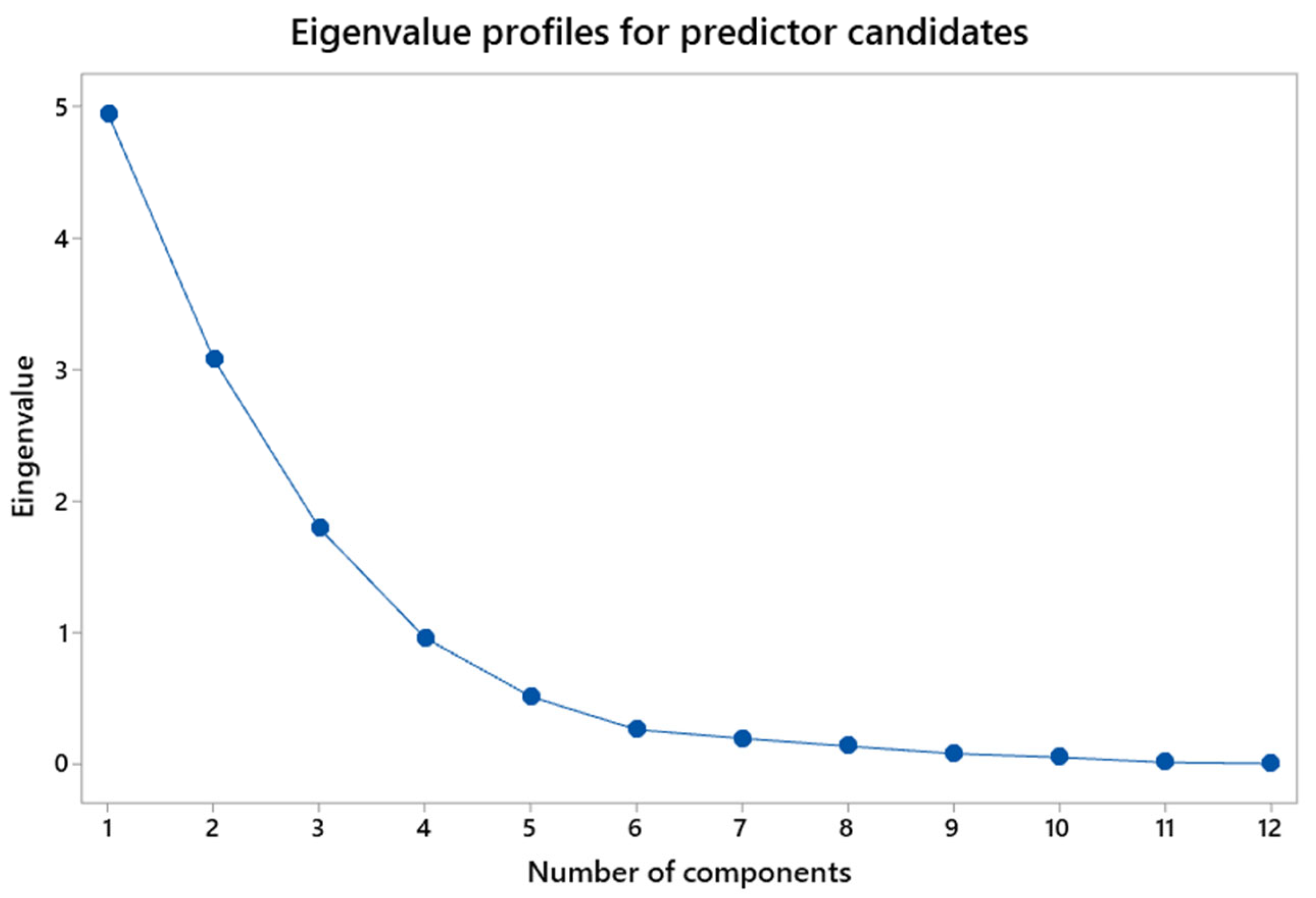
The correlation matrix can also be assessed by Figure 10, where the eigenvalue profiles of the first three components are responsible for explaining 81.9% of the variance. Figure 11 indicates a distribution of predictor candidates regarding their first two components, where some groups of variables can be determined. Three groups can be clearly distinguished: one representing vacuum pressure measurements (PT101, PT125, PT325 and PT225), a second one representing backwash pressure and flow measurements (PT129, PT329, U129_IIT, FT129), and one variable being strongly relevant to component number 2: second-cake-formation valve opening (KPV325). A similar grouping is noted in Table 3.

An iterative procedure was performed to verify the best set of predictors by obtaining multiple regression models with different combinations of predictor groups to obtain the R(t) response. The multicollinearity between predictors was verified and is presented in Table 3, in addition to the p values considering a significance level of 0.05 and the variance inflation factors (VIFs). After three iterations, a model with only four significant variables, with no collinearity effect and with values of VIF sufficiently close to 1 is achieved, presented in

Table 4. Predictor selection for regression model after 3 iterations.

Term	Coef	Coef SE	T Value	p Value	VIF
Constant	−558	533	−1.05	0.303
PT101	8.01	2.21	3.62	0.001	1.42
KPV325	−1.61	0.187	−8.60	0.000	1.22
PT329	−82.0	13.8	−5.96	0.000	1.22
PT129	1073	409	2.63	0.013	1.53

.

Table 5. Analysis of multiple combinations of predictors for R(t) response.

Vars	R2	R2 (aj)	R2 (pred)	Mallow’s Cp	S	U129_IIT	U009_IIT	PT225	PT101	KPV325	PT329	PT129	FT129
4	80.7	78.3	71.4	3.9	5.1743				X	X	X	X
6	82	78.6	57.3	5.7	5.1454			X	X	X	X	X	X
8	82.4	77.6	31.4	9	5.2588	X	X	X	X	X	X	X	X

summarizes the analysis, presenting the coefficients of determination, standard deviation and Mallow’s Cp. The main evaluation criterion is the variation in R², with R²(pred) being the most important of the values, as it reflects the prediction capacity of the model. The Mallow’s CP value is also important in the comparison between models because it evaluates the biases of certain subsets of predictors in the model, having as a goal a value close to the degrees of freedom of the model. The model obtained with four variables presents R² (pred) values that are significantly better than those of the other models and a value of 71.4%, which is considered good for the prediction application of a regression model.

The equation obtained for the regression model for the reliability of ceramic plates is as follows:

R(t) = −558 + 8.01 PT101(t) − 1.610 KPV325(t) − 82.0 PT329(t) + 1073 PT129(t)

The adjusted model had an R² of 80.7%, R²(aj) of 78.3% and R²(pred) of 71.4%.

A qualitative and quantitative evaluation of the model led to the identification of the following factors that affect the reliability of ceramic plates:

• PT101(t)—The loss of vacuum pressure in a vacuum pump. Lower negative vacuum pressures are related to the lower reliability of ceramic plates. The average vacuum pressure loss of 0.1 bar is related to 0.8% lower reliability or, alternatively, a 0.8% increase in the probability of failure.
• KPV325(t)—The higher average second-cake-formation valve opening readings are related to lower reliability values of the ceramic plates. An increase in the average percentage of valve openings by 10% is related to a reliability reduction of approximately 16% or, alternatively, an increase in the probability of failure by 16%.
• PT329(t)—Regarding the variables related to backwash pressure, the higher the average value measured before the bag filter, the lower the reliability of the ceramic plates. A 0.1-bar increase in backwash pressure before the use of the bag filter leads to a reliability reduction of 8.2% or, similarly, an increase in the probability of failure of 8.2%.
• PT129(t)—For the backwash pressure after bag filtration, higher values are associated with higher reliability. The 0.01-bar reduction in the average value of this pressure is related to 10.7% lower reliability or, alternatively, a 10.7% increase in the probability of failure.

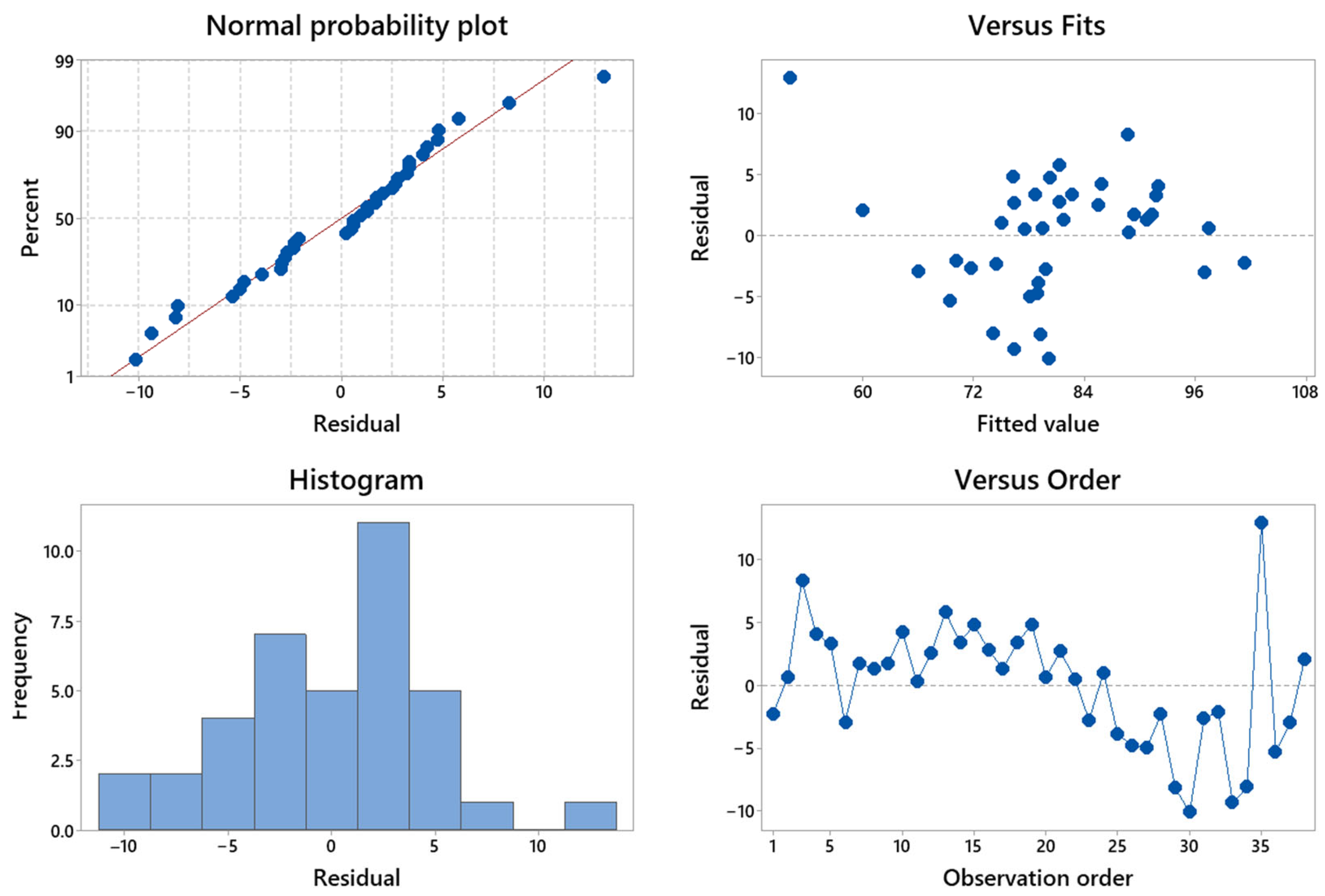
The adequacy of the model is assessed via the residual analysis presented in Figure 12. In the upper-left graph, the residual normal distribution hypothesis is evaluated, whereas a similar visual analysis is also depicted in the histogram graph in the lower-left graph. In both situations, the residuals of the model are well represented by a normal distribution, with a p value of 0.27 in the Anderson–Darling normality test, which fails to reject H₀: the residuals follow a normal distribution. In the upper-right graph of the adjusted value as a function of the residual and in the graph of the observed values as a function of the residuals (lower-right), a reasonably random behavior is observed, with only an apparent trend of lower fit with lower reliability.

The model’s fit with respect to the reliability values R(t), as well as its confidence intervals, is presented in Figure 13. Good adherence to the regression model is observed, which uses only sensor readings to predict the reliability of ceramic plates independently of their operating time. The confidence intervals of some values may contain a fitted reliability higher than 100%, which has no meaning in real-world contexts.

To obtain the remaining useful life, a 70% reliability trigger is obtained at 4822 h of operation. For each instant in time, reliability is calculated from the sensor readings, and the corresponding time of operation is obtained. The remaining useful life is obtained by simply subtracting 4822 h from this result. The equation is expressed as follows:

$$RUL\left(t\right)=4822+\mathrm{13,178}\times \mathrm{l}\mathrm{n}\left[R\right(t\left)\right]$$

Alternatively, it can be replaced with a linear regression model:

$$RUL\left(t\right)=4822+\mathrm{13,178}\times ln[-558+8.01 PT101(t)-1.61 KPV325(t)-82.0 PT329(t)+1073 PT129(t\left)\right]$$

4.4. Random Forest Regression Model for Reliability Prediction

The linear regression model has good predictive ability but uses hourly average data from operating time periods since traditional linear regression models have limitations in the use of large databases. To predict the reliability and remaining useful life in real time, it is necessary to create a model that uses instantaneous data from sensor readings.

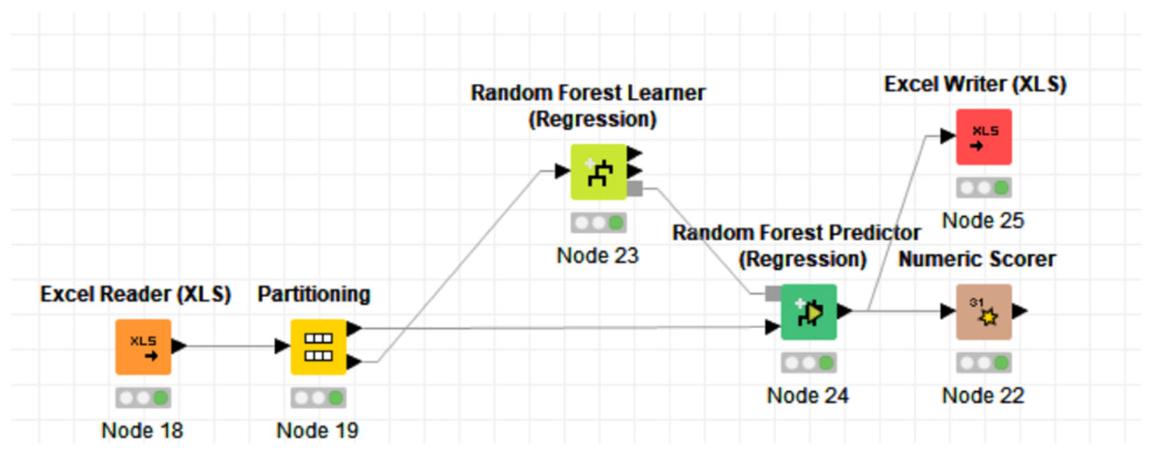
The node layout for the entire model creation process is presented in Figure 14. The first node, identified as Node 18, is responsible for reading the spreadsheet containing the operational data table; then, Node 19 partitions the data into the training set and validation set with a 30%/70% split. The model is created at the node labeled Node 23 using all 12 sensor readings as predictors. Then, on Node 24, using the random partition of 70% of the data as inputs, the reliability prediction is obtained. The evaluation of the model is performed by the statistics obtained from Node 22, and the export of the predicted values is carried out for further analysis at Node 25.

The model obtained was evaluated in relation to the metrics presented in

Table 6. Random forest regression model evaluation.

Metric	Result
R2	0.637
Mean Absolute Error	0.042
Mean Square Error	0.003
Square Root of Mean Square Error	0.056
Average Difference	0

, in which a reasonable R² value was obtained. The model can explain 63.7% of the variation in reliability from the sensor readings used as predictors. The error values are also reasonable for use in prediction.

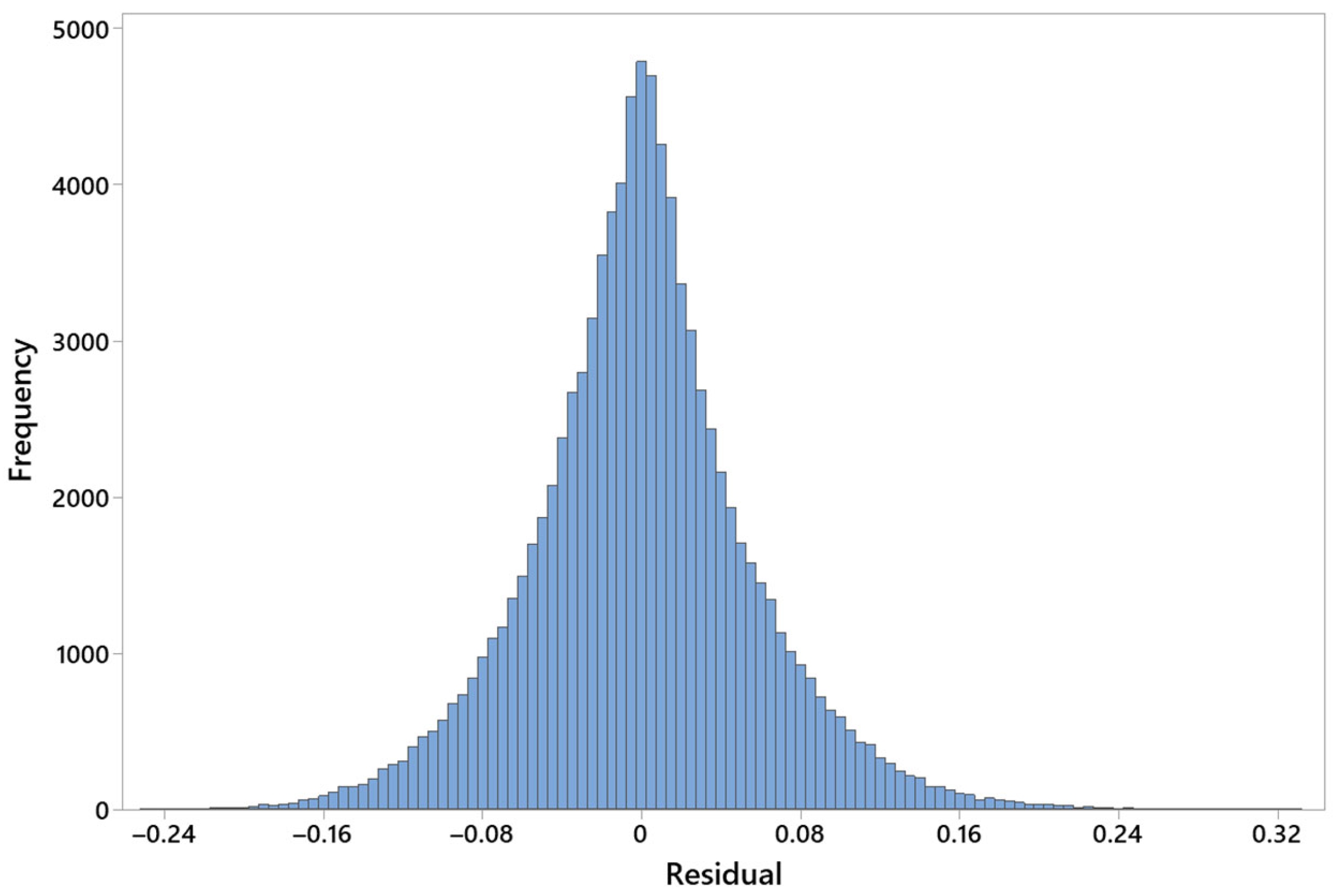
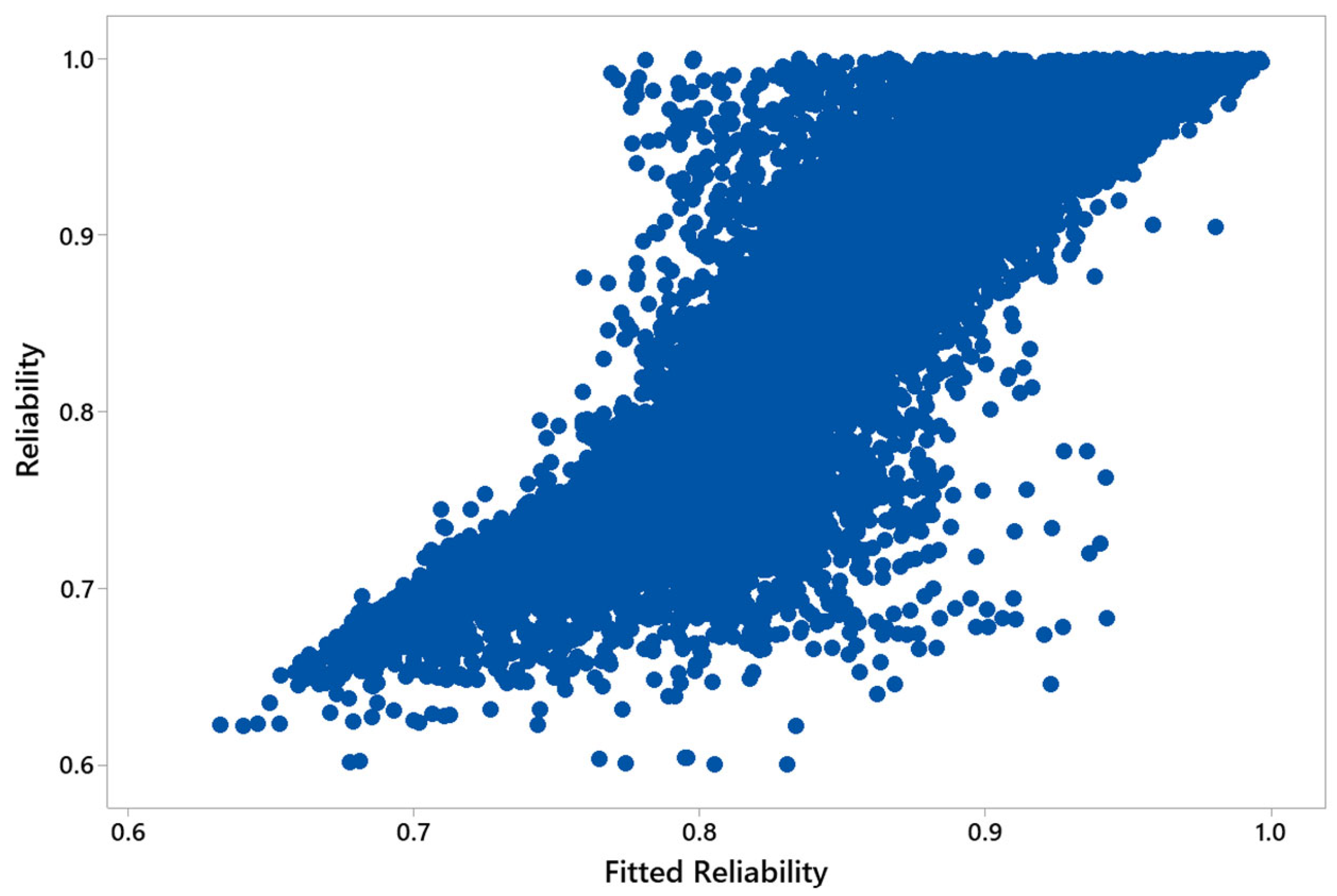
The model is also evaluated in terms of residual distribution, as presented in Figure 15, where an error histogram is displayed. As expected, Figure 16 shows a strong relationship between the actual reliability values and those predicted by the model, with a correlation coefficient of 0.822.

The graph presented in Figure 17 shows a comparison of the estimated reliability and the fitted values. As indicated in Figure 13, although some confidence intervals contain values higher than 100%, they have no meaning in real-world contexts.

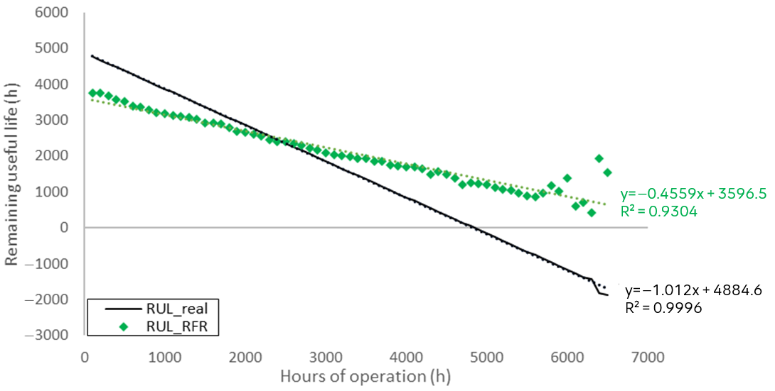
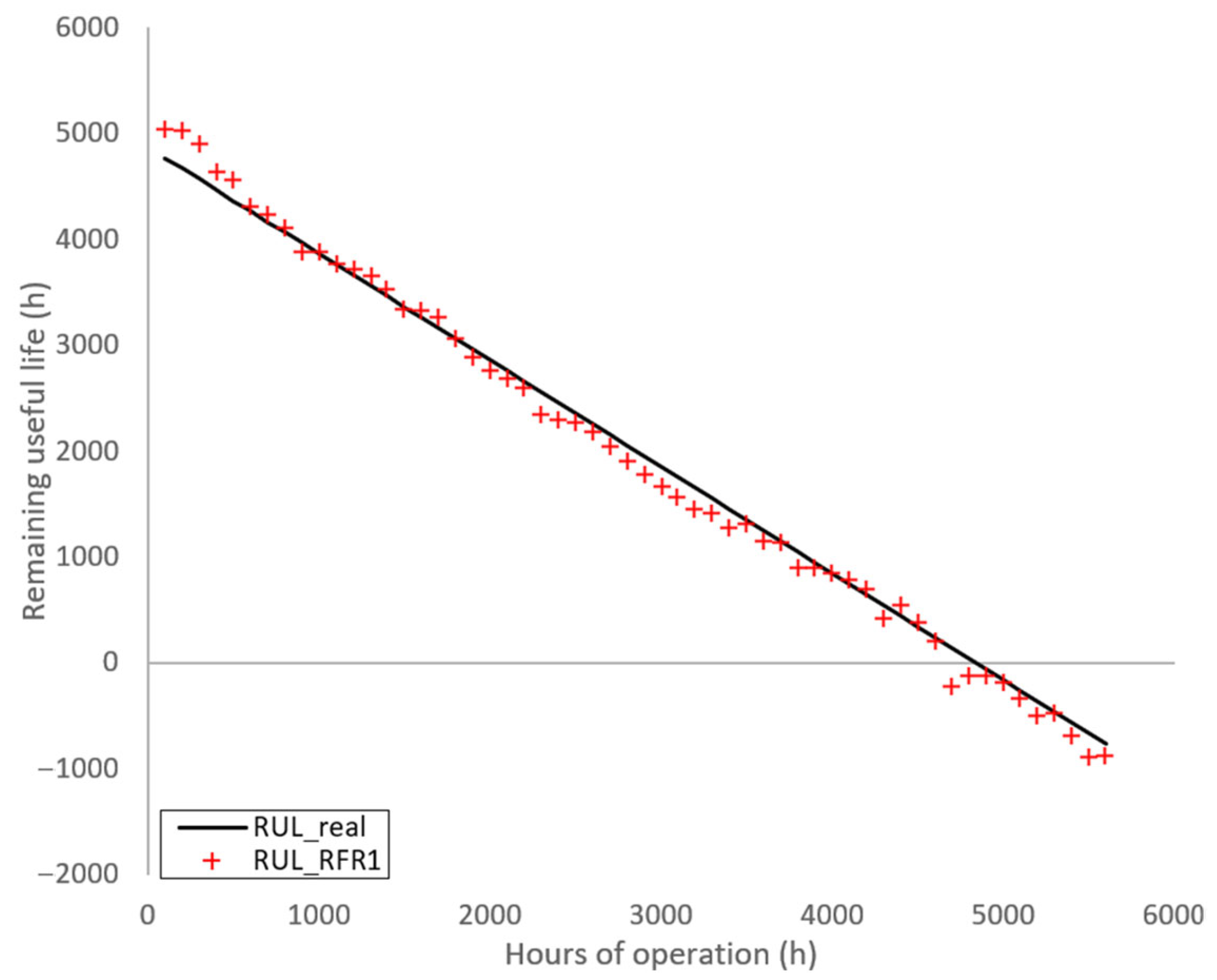
From the reliability estimated by the random forest regression model, a new expression is obtained for the remaining useful life of the ceramic plates. Figure 18 shows a comparison of the results of the analytical reliability model with the results of the fitted model.

For the interval of hours evaluated, it is reasonable to adopt linear models to represent the behavior of the remaining useful life, according to the models and their respective R² values presented in Figure 18. It should be noted, however, that the models do not have the same slope or the same starting point of reliability at 0 hours operated. The linear models of the remaining useful life as a function of time, RUL(t), allow, however, a comparison of the regressions and to stablish an adjustment to the e analytical expression.

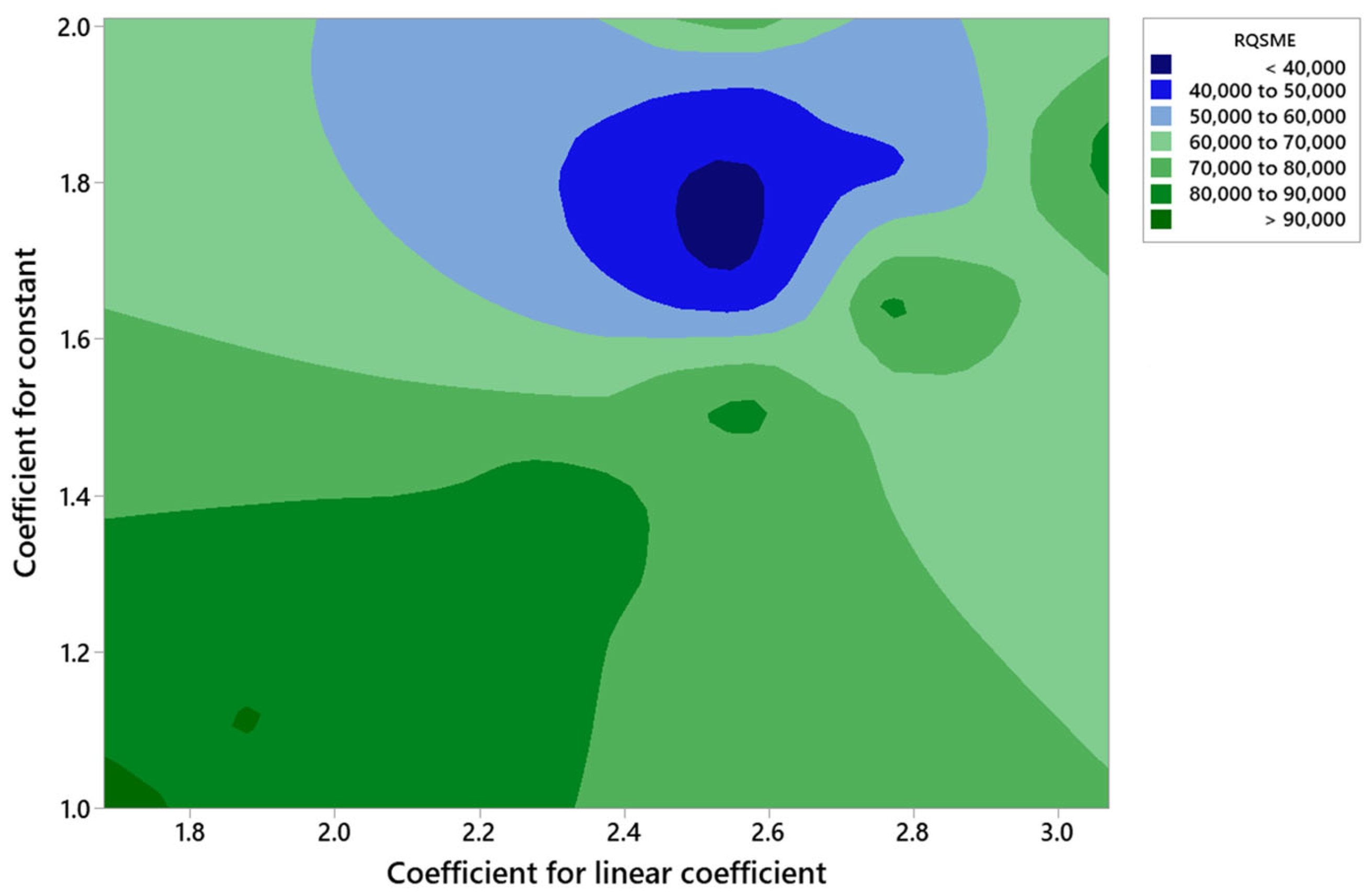
An analysis of the best combination of both the coefficient multiplied by the constant and the slope coefficient is performed to minimize the square root of the mean squared error (RQSME). A contour plot of this analysis is presented in Figure 19, in which the best combination of values is identified as a constant multiplier index of 1.75 and a linear coefficient multiplier index of 2.54.

The results of the training and validation partitions are presented in Figure 20 and Figure 21, respectively. In the adjustment process, the adjustment index of the constant is 1.5, and the adjustment index of the linear coefficient is 2.05. In this scenario, the value of R² was 0.996, and the square root of the mean squared error was 109.96 h. The observation of the model’s limitation in predicting the results of the remaining useful life for operating times greater than 5600 h led to the consideration of only data prior to this interval.

The final model considering the operation of the ceramic plates is given by

$${RUL}_{RFR1}=4822 \times 1.5+\mathrm{13,178} \times 2.05 \times \mathit{ln}\left[{R\left(t\right)}_{estimated}\right]$$

$${RUL}_{RFR1}=7233+\mathrm{27,014.9} \times \mathit{ln}\left[{R\left(t\right)}_{estimated}\right]$$

This is therefore a model capable of predicting, based on only process variables with instantaneous real-time sensor readings, the remaining useful life of ceramic plates operating for up to 5600 h. The final model is independent of operation hours, so if ceramic plates indicate similar operating conditions until the end of life soon after installation, it will be possible to identify this failure and analyze corrections or any early planned replacements. On the other hand, a great gain is that a fixed time for replacing plates is not established, and in the scenario where plates operate beyond their average useful life with good health indicators, users will be able to make the decision to continue operation and monitor the plates’ condition, reducing replacement costs.

The random forest regression model presented together with the developed analytical expression can then be launched in a production environment for performance monitoring with acceptable performance.

5. Conclusions

With the CRISP DM and RUL methodology, it was possible to apply a machine learning model to a case study to predict the remaining useful life of ceramic plates applied in vacuum filters used in the iron ore slurry filtration process.

Data from the automation systems (PIMS and MES) of a real industrial plant were obtained and analyzed. An extensive database with more than 100 thousand operation records, including readings of equipment sensors and records of failures and replacements of ceramic plates for a period of more than 3 years, was analyzed.

To predict reliability as a function of the sensor reading of process variables, mean data were used in a linear regression model, obtaining a model with an R²(pred) of 71.4%. The exponential distribution was used to model the reliability of the ceramic plates over time, considering both failure and preventive replacement of complete plate sets (right-censored data).

The concepts of remaining useful life were used, defining the end of use life based on a 70% reliability trigger. An expression was presented that allows the calculation of the remaining useful life indirectly through the readings of four sensors that act as health indicators of these components in operation in ceramic filters with an R² of 99,6% for up to 5600 h.

The specific goal of this work was achieved by obtaining a predictive model of the probability of ceramic plate failure without the need to install additional sensors.

We highlight the following main contributions:

• The proposed methodology innovates in establishing a link between the CRISP-DM methodology and a methodology for determining the remaining useful life of equipment and components;
• The methodology presented here can be applied to other industrial problems with similar objectives where investment in traditional predictive maintenance sensors (vibration and temperature) is not readily achievable or technically feasible;
• The concept of embedding reliability estimates in PIMSs is not widely applied, even with its high potential. This manuscript can motivate further works considering similar methodologies and environments.

References

1. Kundu, P.; Darpe, A.K.; Kulkarni, M.S. An ensemble decision tree methodology for remaining useful life prediction of spur gears under natural pitting progression. Struct. Health Monit. 2020, 19, 854–872. Available online: https://journals.sagepub.com/doi/10.1177/1475921719865718 (accessed on 7 March 2025). [CrossRef]
2. MATLAB. Predictive Maintenance with MATLAB Ebook Documentation; The MathWorks Inc.: Natick, MA, USA, 2020; Available online: https://www.mathworks.com/content/dam/mathworks/ebook/gated/predictive-maintenance-ebook-all-chapters.pdf (accessed on 18 January 2025).
3. Lei, Y.; Li, N.; Guo, L.; Li, N.; Yan, T.; Lin, J. Machinery health prognostics: A systematic review from data acquisition to RUL prediction. Mech. Syst. Signal Process. 2018, 104, 799–834. Available online: https://linkinghub.elsevier.com/retrieve/pii/S0888327017305988 (accessed on 7 March 2025). [CrossRef]
4. Qin, A.; Zhang, Q.; Hu, Q.; Sun, G.; He, J.; Lin, S. Remaining Useful Life Prediction for Rotating Machinery Based on Optimal Degradation Indicator. Shock Vib. 2017, 2017, 1–12. Available online: https://www.hindawi.com/journals/sv/2017/6754968/ (accessed on 7 March 2025). [CrossRef]
5. Wang, Q.; Zheng, S.; Farahat, A.; Serita, S.; Gupta, C. Remaining Useful Life Estimation Using Functional Data Analysis. In Proceedings of the 2019 IEEE International Conference on Prognostics and Health Management (ICPHM), San Francisco, CA, USA, 17–20 June 2019; IEEE: San Francisco, CA, USA, 2019; pp. 1–8. Available online: https://ieeexplore.ieee.org/document/8819420/ (accessed on 7 March 2025).
6. Liu, G.; Fan, W.; Li, F.; Wang, G.; You, D.; Kastanya, D. Remaining Useful Life Prediction of Nuclear Power Machinery Based on an Exponential Degradation Model. Sci. Technol. Nucl. Install. 2022, 2022, 1–9. Available online: https://www.hindawi.com/journals/stni/2022/9895907/ (accessed on 7 March 2025). [CrossRef]
7. Chu, C.M.; Moon, J.F.; Lee, H.T.; Kim, J. Extraction of Time-varying Failure Rates on power distribution system equipment considering failure modes and regional effects. Int. J. Electr. Power Energy Syst. 2010, 32, 721–727. Available online: https://linkinghub.elsevier.com/retrieve/pii/S0142061510000165 (accessed on 7 March 2025). [CrossRef]
8. Djonglibet, W.-D.; Bianzeube, T.; Ouinra, K. Reliability of Life Calculation Laws for Materials under Variable Amplitude Loading. Open J. Appl. Sci. 2022, 12, 1922–1930. Available online: https://www.scirp.org/journal/doi.aspx?doi=10.4236/ojapps.2022.1211133 (accessed on 7 March 2025). [CrossRef]
9. Santos, L.S.; Pinotti, F.; Luis Duarte Ribeiro, J.; Botelho, H.C. Reliability of Redundant Systems with Repair in an Oil Refinery. Ind. Manag. Mag. 2015, 11, 3. Available online: https://periodicos.utfpr.edu.br/revistagi/article/view/2759 (accessed on 7 March 2025).
10. Hasanain, W.S.; Elaibi, W.M. Reliability Estimation for the Exponential-Pareto Hybrid System. Iraqi J. Sci. 2023, 64, 4622–4633. Available online: https://ijs.uobaghdad.edu.iq/index.php/eijs/article/view/4354 (accessed on 7 March 2025). [CrossRef]
11. Xuegang, L. A Reliability Prediction Method Based on Simulation Analysis. Procedia Eng. 2015, 99, 219–223. Available online: https://linkinghub.elsevier.com/retrieve/pii/S1877705814036431 (accessed on 7 March 2025). [CrossRef]
12. Zhang, C.W.; Zhang, T.; Xu, D.; Xie, M. Analyzing Highly Censored Reliability Data without Exact Failure Times: An Efficient Tool for Practitioners. Qual. Eng. 2013, 25, 392–400. Available online: http://www.tandfonline.com/doi/abs/10.1080/08982112.2013.783598 (accessed on 7 March 2025). [CrossRef]
13. Montgomery, D.C.; Runger, G.C. Applied Statistics and Probability for Engineers, 6th ed.; Technical and Scientific Books: Rio de Janeiro, Brazil, 2016. [Google Scholar]
14. Bokrantz, J.; Subramaniyan, M.; Skoogh, A. Realizing the promises of artificial intelligence in manufacturing by enhancing CRISP-DM. Prod. Plan. Control 2024, 35, 2234–2254. Available online: https://www.tandfonline.com/doi/full/10.1080/09537287.2023.2234882 (accessed on 7 March 2025). [CrossRef]
15. Doede, N.; Merkel, P.; Kriwall, M.; Stonis, M.; Behrens, B.-A. Implementation of an intelligent process monitoring system for screw presses using the CRISP-DM standard. Prod. Eng. 2025, 19, 77–88. Available online: https://link.springer.com/10.1007/s11740-024-01298-8 (accessed on 7 March 2025). [CrossRef]
16. Wiemer, H.; Drowatzky, L.; Ihlenfeldt, S. Data Mining Methodology for Engineering Applications (DMME)A Holistic Extension to the CRISP-DM Model. Appl. Sci. 2019, 9, 2407. Available online: https://www.mdpi.com/2076-3417/9/12/2407 (accessed on 7 March 2025). [CrossRef]
17. Gayathri, R.; Rani, S.U.; Čepová, L.; Rajesh, M.; Kalita, K. A Comparative Analysis of Machine Learning Models in Prediction of Mortar Compressive Strength. Processes 2022, 10, 1387. Available online: https://www.mdpi.com/2227-9717/10/7/1387 (accessed on 7 March 2025). [CrossRef]
18. Tayade, A.; Patil, S.; Phalle, V.; Kazi, F.; Powar, S. Remaining useful life (RUL) prediction of bearing by using regression model and principal component analysis (PCA) technique. Vibroeng. Procedia 2019, 23, 30–36. Available online: https://www.extrica.com/article/20617 (accessed on 7 March 2025). [CrossRef]
Figure 1. Illustration of maintenance strategies [2]: reactive maintenance (left), preventive maintenance (middle) and predictive maintenance strategies (right).
Applsci 15 08081 g001
Figure 2. Ways to estimate remaining useful life [2].
Applsci 15 08081 g002
Figure 3. Schematic diagram of the CRISP-DM process [15].
Applsci 15 08081 g003
Figure 4. Random forest regression methodology [1].
Applsci 15 08081 g004
Figure 5. Methodology applied in research.
Applsci 15 08081 g005
Figure 6. New ceramic plate (left) and filter in the process of replacing a plate set (right). Written on its bottom part, the new plate has “Outotec” (manufacturer), “Red 30 Plate” (type of ceramic plate), an arrow indicating the “Direction of Rotation” and numbers identifying the serial number and batches.
Applsci 15 08081 g006
Figure 7. Examples of failure modes in ceramic plates: cracked and broken plates.
Applsci 15 08081 g007
Figure 8. Distribution of the time intervals of complete ceramic plate set renewals.
Applsci 15 08081 g008
Figure 9. Exponential model for ceramic plate failure data.
Applsci 15 08081 g009
Figure 10. Eingenvalue profiles for predictor candidates.
Applsci 15 08081 g010
Figure 11. Loading plot of predictor candidates.
Applsci 15 08081 g011
Figure 12. Residual analysis of the regression model.
Applsci 15 08081 g012
Figure 13. R(t) and adjusted values with 95% confidence intervals (CIs). Y-axis ranges from 30% to 120% for improved visualization only.
Applsci 15 08081 g013
Figure 14. Node layout for creating a random forest regression model. Arrows indicate the data flow from nodes; each node ha its inputs on the left and outputs on the right. The square end line indicates that the model created at Node 23 is used as an input at Node 24 for random forest prediction.
Applsci 15 08081 g014
Figure 15. Histogram of the model residuals in relation to the estimated reliability.
Applsci 15 08081 g015
Figure 16. Scatter plot of reliability versus predicted reliability.
Applsci 15 08081 g016
Figure 17. Comparison of reliability versus values predicted by the random forest regression model. Y-axis ranges from 30% to 120% for improved visualization only.
Applsci 15 08081 g017
Figure 18. Comparison between actual remaining useful life and fitted model.
Applsci 15 08081 g018
Figure 19. RQMSE contour plot as a function of the coefficients of the fit of the constant and the linear coefficient.
Applsci 15 08081 g019
Figure 20. Comparison between actual remaining useful life and fitted training model.
Applsci 15 08081 g020
Figure 21. Comparison between actual remaining useful life and fitted validation model.
Applsci 15 08081 g021