A Comparative Analysis of Machine Learning Models in Prediction of Mortar Compressive Strength

Abstract

Predicting the mechanical properties of cement-based mortars is essential in understanding the life and functioning of structures. Machine learning (ML) algorithms in this regard can be especially useful in prediction scenarios. In this paper, a comprehensive comparison of nine ML algorithms, i.e., linear regression (LR), random forest regression (RFR), support vector regression (SVR), AdaBoost regression (ABR), multi-layer perceptron (MLP), gradient boosting regression (GBR), decision tree regression (DT), hist gradient boosting regression (hGBR) and XGBoost regression (XGB), is carried out. A multi-attribute decision making method called TOPSIS (technique for order of preference by similarity to ideal solution) is used to select the best ML metamodel. A large dataset on cement-based mortars consisting of 424 sample points is used. The compressive strength of cement-based mortars is predicted based on six input parameters, i.e., the age of specimen (AS), the cement grade (CG), the metakaolin-to-total-binder ratio (MK/B), the water-to-binder ratio (W/B), the superplasticizer-to-binder ratio (SP) and the binder-to-sand ratio (B/S). XGBoost regression is found to be the best ML metamodel while simple metamodels like linear regression (LR) are found to be insufficient in handling the non-linearity in the process. This mapping of the compressive strength of mortars using ML techniques will be helpful for practitioners and researchers in identifying suitable mortar mixes.

1. Introduction

Rapid urbanization throughout the globe has increased the demand for construction materials. Concrete is perhaps the most widely used artificial material in the construction industry. However, the recent impetus of the world towards finding sustainable and eco-friendly means of construction has led to a lot of research on improving concretes and trying to reduce their adverse impact on the earth. Many researchers in this regard suggest the use of metakaolin (MK) as a partial replacement for Portland cement [1]. MK is obtained by high-temperature (700–900 °C) calcination of silica and alumina. Khatib et al. [2] suggest that MK can be used to replace some amount of cement in mortars, resulting in significant improvement in the mechanical performance of concretes. It has been reported by other researchers as well that the addition of MK can help in the improvement of the compressive strength (CS) of mortars [3].

Some analytical formulas have been derived by researchers for estimating the CS of mortars [4]. However, these analytical relations are difficult to derive when MK is present in the mortars. Significant non-linearity has been reported by researchers in such cases, making simple statistical models like response surface methodology insufficient. Machine learning (ML) metamodels are viable alternatives in such cases. Among various ML methods, artificial neural networks (ANN) have received a lot of attention in this field. Onal and Ozturk [5] tried to derive a cause–effect synergy between microstructural characteristics and CS of cement mortars. They relied on ANN metamodels and found that CS and microstructural characteristics share a strong correlation. Asteris et al. [6] employed ANN to estimate the mortar compressive strength based on its mixed components. Eskandari-Naddaf and Kazemi [7] used ANN to predict the compressive strength of cement mortar. They carried out experimental verification for their ANN metamodels and concluded that the cement strength class is also a significant input parameter and thus should be included in data-driven methods. Sharifi and Hosseinpour [8] developed a new formula to express the CS as a function of input parameters by using ANN metamodels.

Some researchers have also relied on metaheuristic algorithms to train and enhance the ANNs. For example, Asteris et al. [9] in a recent study used metaheuristic algorithms like biogeography-based optimization (BBO) and invasive weed optimization algorithms to train ANN for predicting the CS of mortars. Ly et al. [10] used a particle swarm optimization (PSO) algorithm to train ANNs in the prediction of CS for foamed concrete. They showed the PSO-trained ANN to be significantly better than vanilla ANN. Zhao et al. [11] used BBO and a multi-tracker optimization algorithm to enhance the performance of ANN in prediction tasks of the CS of manufactured-sand concrete. A similar attempt was made by Sun et al. [12] by incorporating an artificial bee colony algorithm to train the hyperparameters of ANN.

The majority of the literature on the estimation of the CS of mortars is seen to be focused on the use of ANNs. In some cases, researchers have compared the performance of ANNs with other MLs. For example, Armaghani and Asteris [13] compared ANN metamodels with ANFIS metamodels for the prediction of the CS of mortars and reported that ANFIS metamodels were prone to overfitting in some cases. Sevim et al. [14] too compared the utility of ANFIS and ANN in such applications. Asteris et al. [15] used ANN and genetic programming (GP) metamodels for estimating the 28-day CS of cement–metakaolin mortars. They found ANNs to be superior to the GP metamodels. Dao et al. [16] compared several Gaussian process regression (GPR) metamodels with ANN metamodels and reported that the GPR metamodel with a Matern32 kernel function outperforms others. Mohammed et al. [17] carried out a comparison of ANN, M5P trees and non-linear regression methods. They found curing time to be the most important input parameter in estimating the CS of mortars. Similarly, Abdalla and Salih [18] compared M5P trees, GP and ANN metamodels.

Comparison studies on the application of ML algorithms other than ANNs for the estimation of the CS of cement mortars are relatively fewer. Asteris et al. [19] in a recent study compared the performance of k-nearest neighbors (kNN), decision tree regression (DT), support vector regression (SVR), random forest regression (RFR) and AdaBoost regression (ABR) algorithms. They reported RFR and ABR algorithms to be the most apt for the task. Çalışkan et al. [20] compared group methods of data handling, SVR and extreme learning machine (ELM) and found ELM to outperform the other two metamodels. Ozcan et al. [21] used SVR, RFR, ABR and Bayes classifier to develop estimation metamodels for CS based on four input parameters.

From the above literature survey, it is observed that most of the researchers have mostly relied on ANNs for the prediction modelling of the CS of mortar mixes. Very few comparative studies of ML techniques have been carried out, but they too have generally compared only two to three ML techniques. Thus, there is a literature gap in terms of a comprehensive comparison of ML techniques. In this paper, nine popular ML methods (namely, linear regression (LR), RFR, SVR, ABR, multi-layer perceptron (MLP), gradient boost regression (GBR), DT, hist gradient boost regression (hGBR) and XGBoost regression (XGB)) have been compared for developing metamodels for the CS of mortar mixes. The hyperparameters of the metamodels are tuned for unbiased comparison.

2. Machine Learning Methods

2.1. Linear Regression

Linear regression (LR) is a statistical method widely used for analyzing the effect of input (independent) and output (dependent) variables. Recently it has been widely implemented in various machine learning libraries and thus has become extremely popular as a machine learning algorithm [22].

LR is capable of deriving linear models, i.e., a model that establishes the dependent variable ($y$) as a linear function of the independent variables ($x$). In simple LR, only one independent variable ($x$) is present, whereas in multiple LR, two or more independent variables ($x$) are present. In simple LR, the model is of the following form:

$$y =b_{ 0} + b_{ 1} x$$

(1)

Equation (1) above represents the equation of a straight line, where $b_{ 0}$ and $b_{ 1}$ are the $y$-intercepts and the slope, respectively.

In multiple LR, instead of the line, a plane or a hyper-plane is used. The model takes the following form in multiple LR:

$$y = b_0 + b{ }_{1}x{ }_1 + b_{ 2}{x}_{ 2} + b{ }_3{x}_{ 3} + \dots + b{ }_{n}x{ }_n$$

(2)

In Equation (2), there are $n$ number of predictors ($x_1,x_2,\dots ,x_n$).

2.2. Random Forest Regression

The random forest algorithm is an ensemble technique. It can be employed to perform both regression and classification. The random forest algorithm uses simple decision trees as the base learners [23]. It employs many decision trees to generate a model for the problem. It trains multiple trees simultaneously by using the technique of bootstrap aggregating or bagging. From a given set of training data $\left(X\right)$, bagging techniques repeatedly select $B$ number of times random samples (with replacement) of training data and trains the decision trees. These decision trees do not interact with each other during the building phase and are generated parallelly. Once trained, these trees can be used to predict the unknown samples $\left(x^{\prime }\right)$ by using the following equation:

$$\widehat{f}=\frac{1}{B}{\displaystyle \sum }_{b=1}^B{f}_b\left(x^{\prime }\right)$$

(3)

In general, the decision trees have high variance. However, when they are combined parallelly to form the random forest, the overall variance becomes low. During classification tasks, the random forest algorithm uses the mode of the classes, whereas during regression, it uses the mean of decision trees.

2.3. Support Vector Regression

Support vector machine (SVM) can be employed for both regression and classification tasks [24]. The prime objective of SVM is to generate the best decision boundary that can separate $n$-dimensional space into distinct classes. In SVM, the best decision boundary is referred to as a hyperplane. The algorithm chooses support vectors which can then aid in the creation of the hyperplane. SVM can be linear or non-linear. If the data is linearly separable, linear SVM is used. In such cases, the data can be segregated into two classes by a straight line. In cases when the data cannot be segregated by using a single straight line, non-linear SVM is used.

2.4. AdaBoost Regression

AdaBoost or adaptive boosting is an ensemble technique. AdaBoost works by conjugating several weak learners into a single strong learner. Generally, AdaBoost uses single split decisions, called decision stumps, as the weak learners [25]. AdaBoost allocates weights to the classification instances depending on the difficulty level, i.e., instances that are difficult to classify are allocated higher weights than those instances that are easy to classify. Adaptive boosting can be employed for both regression and classification tasks.

Switching from LR to AdaBoost allows mapping of many more non-linear relationships, which results in better estimation and, thus, higher accuracy. As a general principle, AdaBoost builds ensembles by sequentially adding members which have been trained on those instances of data which are proving the most difficult to correctly predict. Each new predictor is given a training set where the difficult examples are increasingly represented; this is achieved either through weighting or resampling.

An ABR is a meta-estimator which initiates by training a regressor on the training dataset and then trains further replicas of the regressor on the training data. However, in the training of the subsequent regressors, weights of instances are attuned depending on the error encountered in the current regressor. Thus, successive regressors attain more accuracy by focusing more on difficult cases.

2.5. Multi-Layer Perceptron

Multi-layer perceptron (MLP) is a machine-learning and deep-learning method that defines a complex architecture for artificial neural networks [26]. The method is generally used for the supervised learning format. MLP is typically a feed-forward neural network which produces a set of output from a set of input. It is broadly created from several layers of the perceptron. The multiple layers of input nodes are linked just like a directed graph. In MLP, the adaline rule and perceptron rule are used in training a neural network of a single layer, and weights are updated based on the unit function on a linear function in the adaline or perceptron rule.

An MLP is a fully linked neural network. It consists of three layers which include a hidden layer. When there is more than one hidden layer, it is referred to as a deep artificial neural network (ANN). The number of neurons and the number of layers are the ones that require tuning. To find the ideal values for the hyperparameters (number of neurons and number of layers), cross-validation approaches are employed. Backpropagation assists in training weight adjustments.

The MLP approach involves three steps:

• Forward propagation—data propagation begins at the input layer and forwards to the output layer;
• Error calculation—find the error (variation between the estimated and known outcomes) based on the output;
• Backpropagate the error—the derivative based on respective weights in the network is determined, and then the model is updated.

The steps are repeated across multiple epochs to establish ideal weights, and then the output is taken through a threshold function to get the estimated class labels.

2.6. Gradient Boosting Regression

Gradient boosting is an ensemble technique. It is primarily used for regression tasks. The method works on the boosting principle where several weak learners are conjugated to form a strong learner. Generally, decision trees are used as the weak learners. First, base trees with single nodes are constructed. Subsequent trees are constructed depending on the errors of the previous trees. The trees are scaled by using the learning rate, which ensures the contribution of each tree to the overall prediction. The subsequent trees are joined with the preceding trees to predict the response. The process is repeated unless the maximum number of trees is reached or the resulting responses are not improved [27].

Gradient boosting regression can help in expressing dependent variables as functions of independent variables. GBR can be used for the prediction of the numeric output; thus, the response variable should be numeric.

2.7. Decision Tree Regression

Decision tree regression uses the characteristics of an object to train a model within the tree structure to estimate future data to generate meaningful continuous data. It encompasses interrogating the data through a series of questions with each question narrowing the possible values until a confident model is developed. The decision tree regression decomposes a given dataset into smaller datasets. It consists of a decision leaf that splits into two or more branches which present the value of the attribute that is being examined. The node that is at the top, i.e., topmost, is the most suitable predictor, and it is referred to as the root node. The decision tree regression technique uses a top–down tactic. Splits are made based on standard deviation. When a sample is entirely homogenous, its standard deviation is 0, whereas when the standard deviation is greater, it implies that the degree of homogeneity is higher [28].

Decision tree regression generally uses mean squared error (MSE) to decide on splitting a node into two or more sub-nodes. In decision tree regression, the way to find the best split is to try each variable and every potential value of the given variable and identify the variable and value that give a split with the best score.

2.8. Hist Gradient Boosting Regression

Hist gradient boosting regression is a method for training faster decision trees employed in gradient boosting. Binning or discretizing can be used to dramatically speed up the process of training trees which are added to an ensemble. This makes the hist gradient boosting method implement its algorithm for the input variables. Each of the trees that are added to an ensemble tries to correct the forecasted errors through the models that already exist in the ensemble.

The hGBR technique is implemented along with other techniques. For example, it can be implemented with the scikit-learn machine learning, which is a library that gives an experimental implementation of gradient boosting which underpins the histogram approach. In particular, it provides the HistGradientBoostingRegressor and HistGradientBoostingClassifier classes. According to the scikit-learn documentation, hGBR implementation has faster orders of magnitude compared to the default GBR implementation offered by the library.

2.9. XGBoost Regression

XGBoost or extreme gradient boosting is a popular and powerful ML technique for building supervised regression models [29]. XGB is highly efficient and computationally effective. It has remarkably higher accuracy than decision trees but lacks the interpretation ability of decision trees. Base learners are needed in XGB. The algorithm trains and keeps on adding base learners to form an ensemble learning which then can perform the prediction. The objective function of the XGB contains a regularization term and the loss function. The variation in the target values and the predicted values, i.e., the variation between the model predictions and actual values, is known using the objective function.

3. Problem Description

The compressive strength of cement-based mortars is the most important property to be considered while selecting the appropriate mixture for construction. A large experimental dataset on cement-based mortars is collected from the literature [19]. This dataset has 424 data points generated experimentally by 20 different research studies [1,30,31,32,33,34,35,36,37,38,39,40,41,42,43,44,45,46,47,48]. However, all these studies have followed the same testing standards. The dataset contains information about the CS of mortar mixes with and without MK. In addition, superplasticizers (SP) are present in some of the experiments. The dataset has six different input parameters, namely the age of specimen (AS), the cement grade (CG), the metakaolin-to-total-binder ratio (MK/B), the water-to-binder ratio (W/B), the superplasticizer-to-binder ratio (SP) and the binder-to-sand ratio (B/S). The AS is measured in days, while CG and CS are measured in MPa. The MK/B, W/B, SP and B/S are measured as w/w. It should be noted that one of the most prominent features of the dataset is the inclusion of CG, which, despite being an important input parameter, has often been missed by previous computational modelling studies [19]. The objective of this computational modelling study is to use the ML algorithms in developing metamodels to express the CS as a function of the six input parameters.

4. Results and Discussion

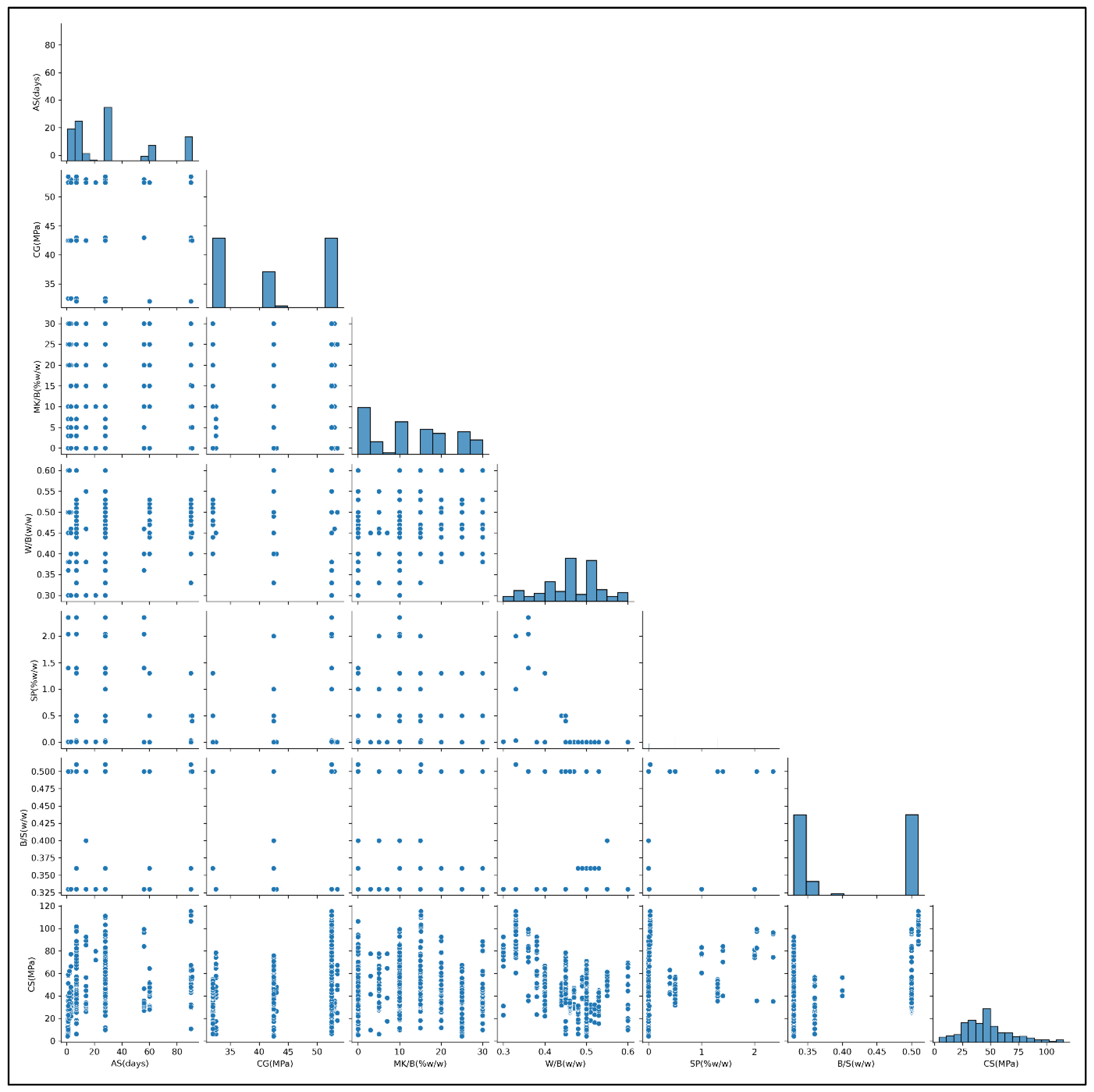
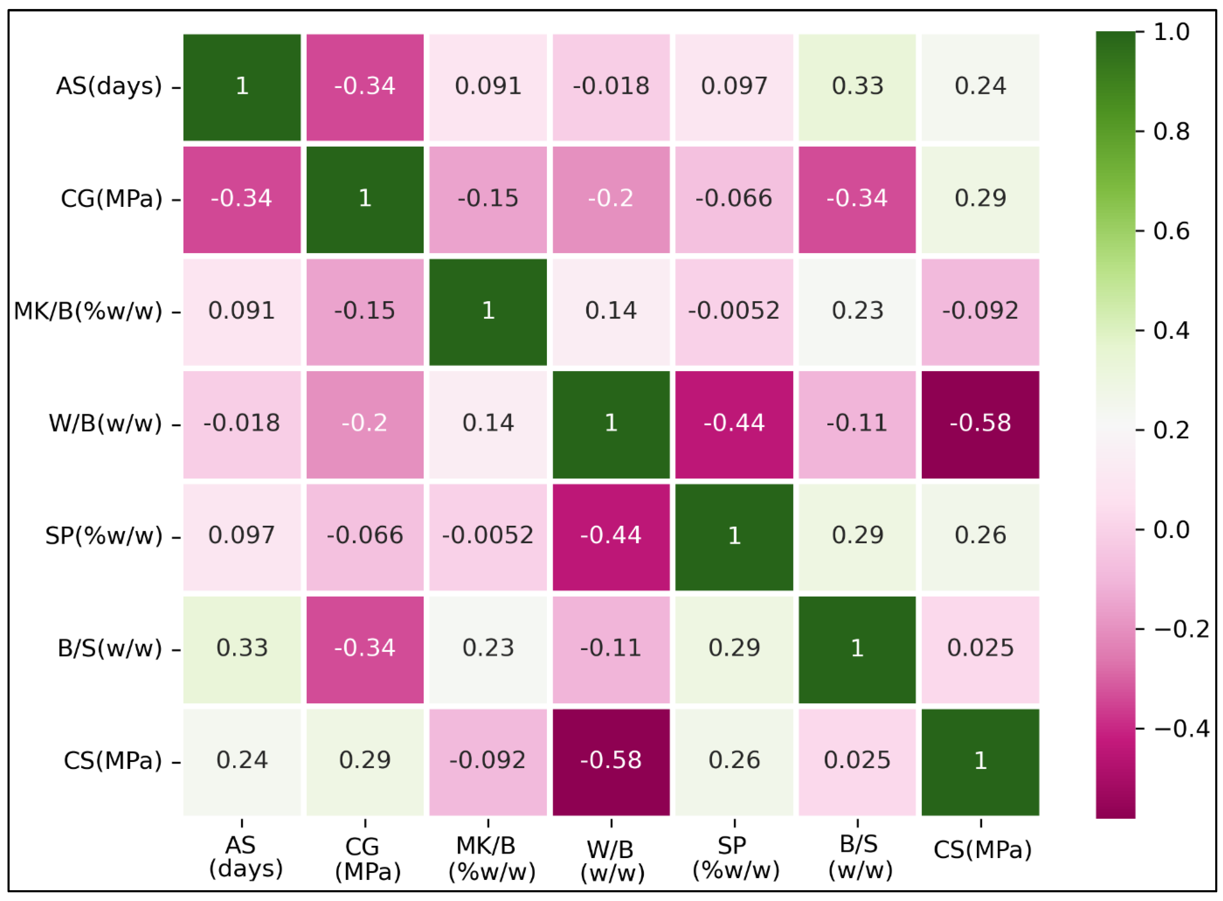
4.1. Characteristics of the Cement-Based Mortars Database

The collated database is analyzed to reveal the statistical characteristics (

Table 1. Statistical summary of the dataset.

Statistic	AS (Days)	CG (MPa)	MK/B (w/w)	W/B (w/w)	SP (w/w)	B/S (w/w)	CS (MPa)
Count	424	424	424	424	424	424	424
Mean	29.80981	42.39151	12.39811	0.457476	0.208325	0.411132	46.42219
Std	29.28965	9.151924	10.00436	0.069217	0.493958	0.083049	21.79888
Min	0.67	32	0	0.3	0	0.33	4.1
25%	7	32	0	0.4	0	0.33	31.1675
50%	28	42.5	10	0.46	0	0.36	44.315
75%	28	52.5	20	0.5	0.01	0.5	56.76
Max	91	53.5	30	0.6	2.35	0.51	115.25

) of all the input and output parameters. The range of the CS of the tested mortar mixes is found to be between 4.1 MPa and 115.25 MPa, which indicates the diversity in the test samples considered in the dataset. Figure 1 contains pair plots that show the level-wise spread of the data points. It is observed that the dataset contains CS values for only five possible binder-to-sand ratios (B/S). The range of the B/S in the dataset varies from 0.33 to 0.51, indicating that researchers agree that typically a binder-to-sand ratio of 1:3 or 1:2 is desirable. Similarly, from Figure 1, it is observed that the experimental dataset contains CS values for only seven possible cement grades (CG). Despite this, a close investigation of the CG pair plot indicates that the researchers prefer CG in three distinct zones, i.e., low (~32 MPa), mid (~42 MPa) and high (~53 MPa).

To check for multicollinearity, the Pearson’s correlation coefficients are computed for the input and the output parameters and presented as a heatmap in Figure 2. The relatively strongest correlation coefficient between any two inputs is seen for the water-to-binder ratio (W/B) and the superplasticizer-to-binder ratio (SP) at −0.44, indicating a weak negative correlation. The other inputs share weak to negligible correlations amongst themselves. The strongest relation between any input and CS is seen for the water-to-binder ratio (W/B) and CS at −0.58.

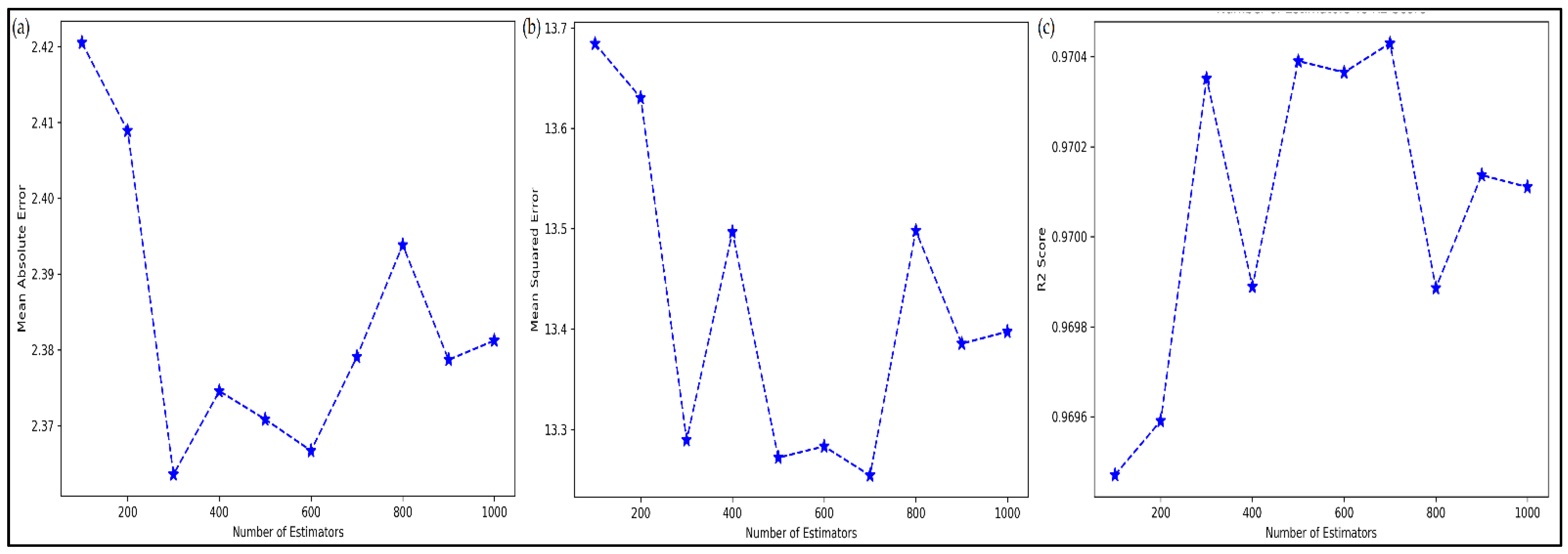
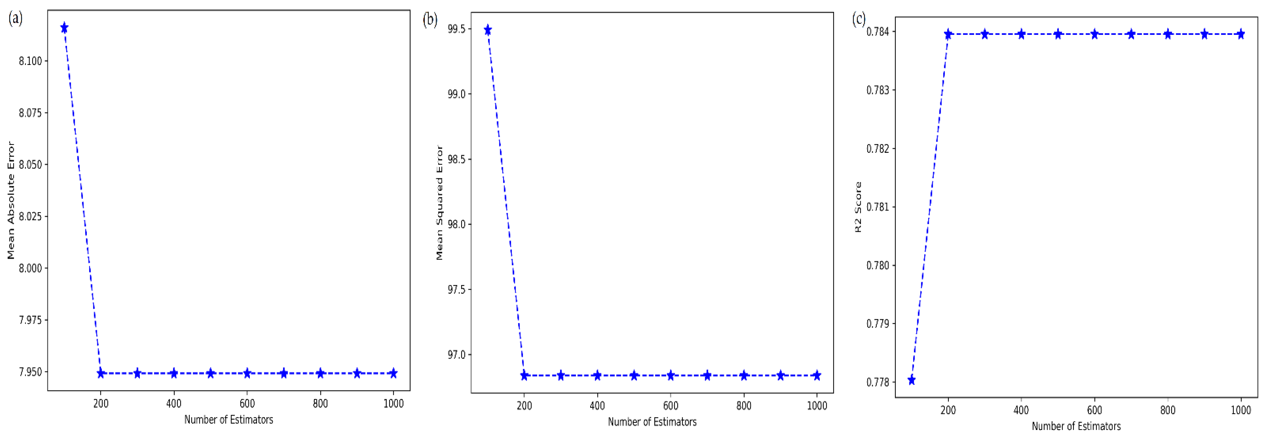
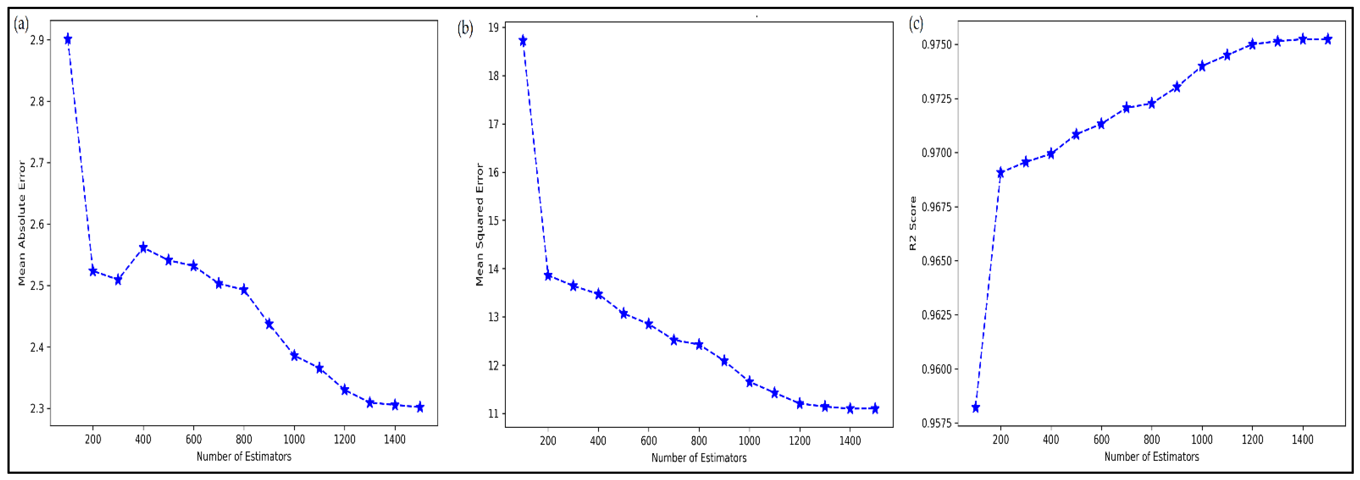
4.2. Tuning of ML Metamodels

The ML metamodels are initially tuned to optimize the most prominent hyperparameters. This is done by varying the number of estimators and training the ML metamodels. These trained ML metamodels are then tested on the test dataset, and their MAE, MSE and $R^2$ are recorded and analyzed. Figure 3 shows the effect of the number of estimators in RF on the accuracy of the metamodel. It is seen that the effect is quite non-linear and, thus, underlines the fact that the number of estimators in RF cannot be set arbitrarily without carrying out a pilot study. The MAE of RF is found to be lowest at 300 estimators while MSE is lowest at 700 estimators. The $R^2$ of RF is found to be highest at 700 estimators, and thus, it is selected for the study.

In Figure 4, the effect of change in estimators on the AdaBoost accuracy is analyzed and found that 200 estimators are sufficient. Similarly, in Figure 5 for MLP, the improvement in its performance is found to be directly related to the number of perceptrons used. However, beyond a threshold, the rate of improvement is found to be negligible. Thus, for further analysis in the study with MLP, the number of perceptrons is fixed at 2750.

In the case of GBR, as shown in Figure 6, the metamodel’s accuracy is seen to be quite significantly affected by the number of estimators. For GBR, 1400 estimators were found to be the most optimized value for maintaining the high accuracy of the metamodel.

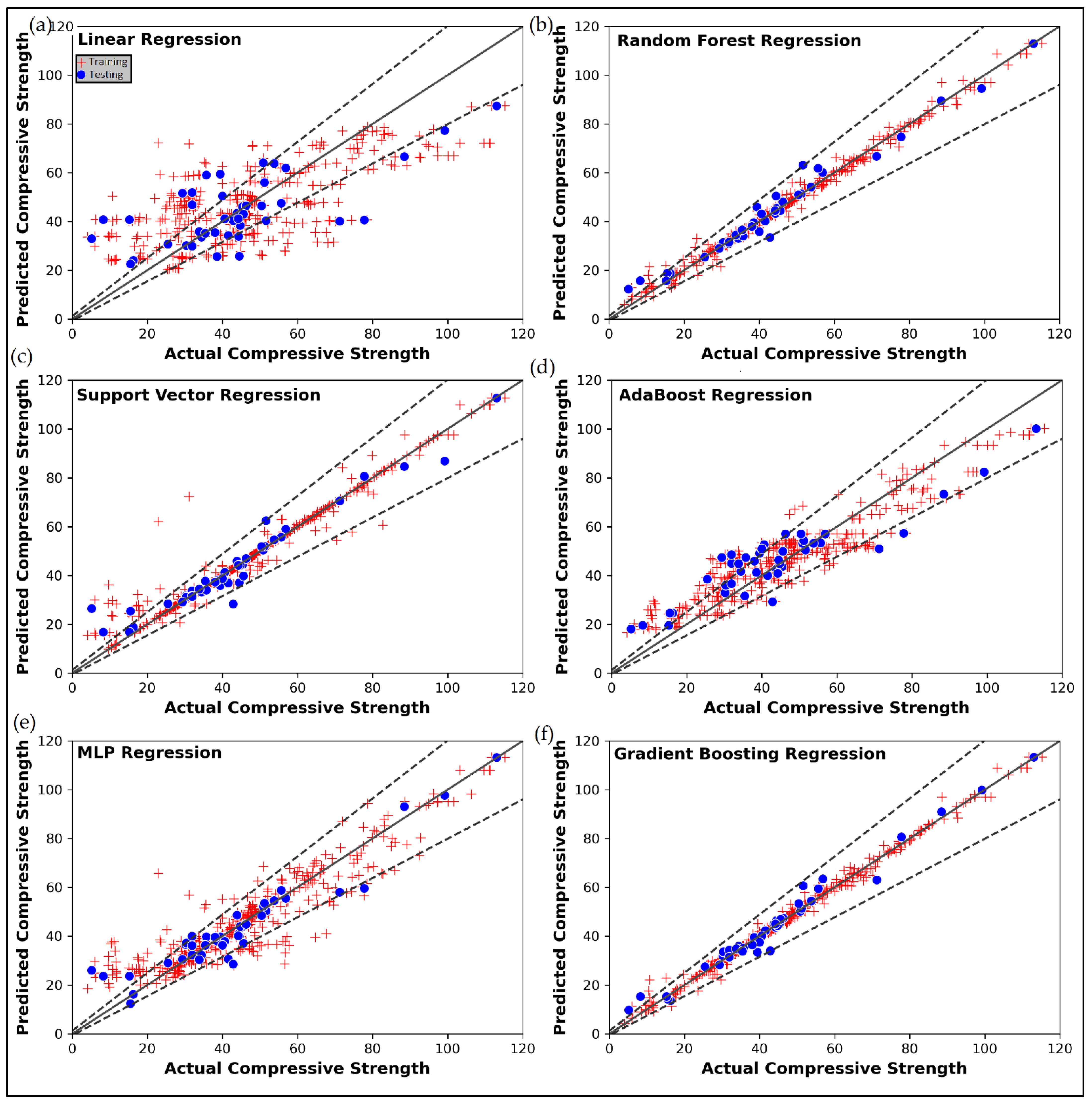
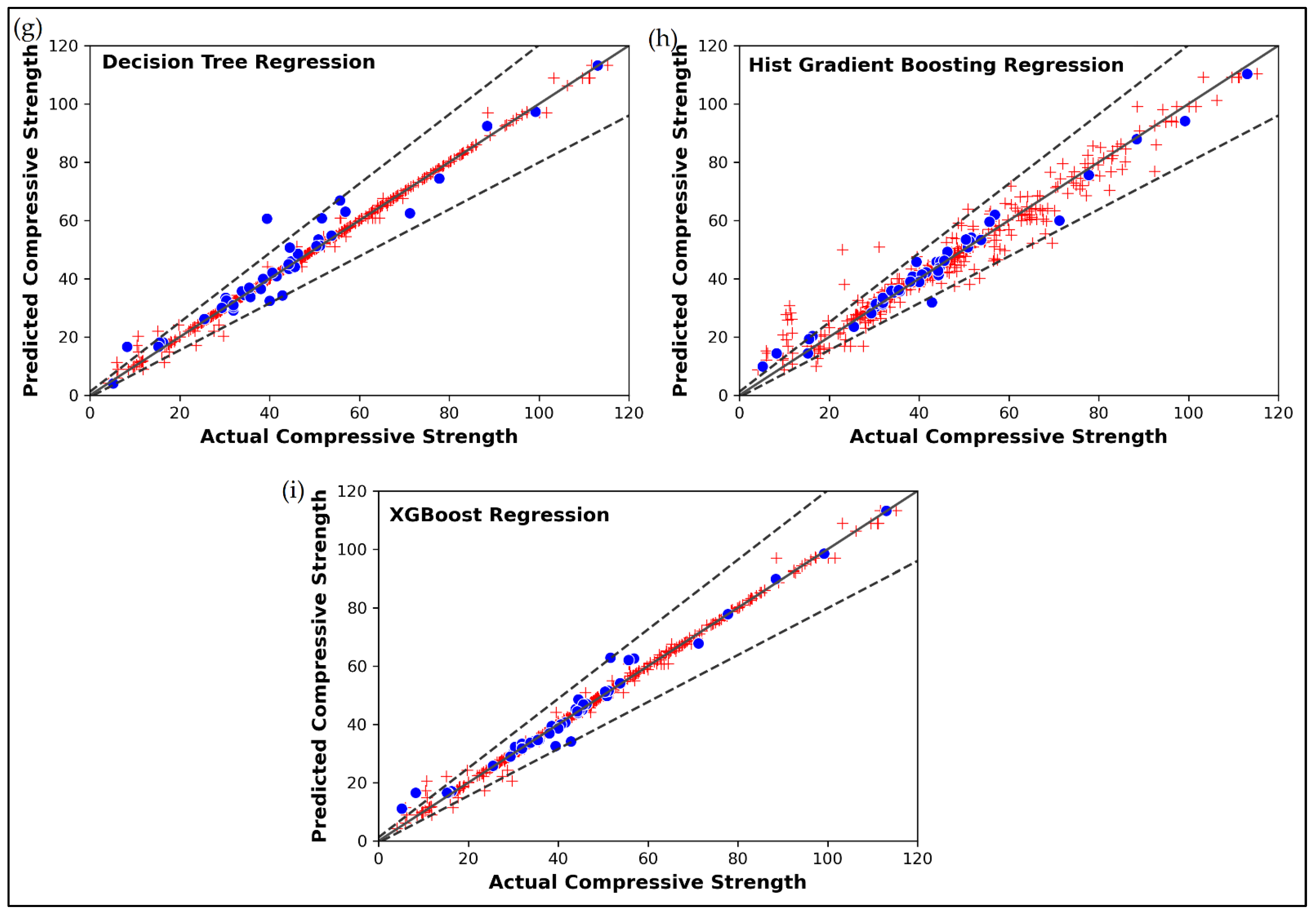
4.3. Prediction of Cement-Based Mortars’ Compressive Strength

The tuned ML metamodels are then deployed on the collated dataset to predict the CS of mortar mixes. The scatter plots of the actual versus the ML predictions are plotted in Figure 7 for both training and testing data. The prediction scatter by LR in Figure 7a shows that these simple linear metamodels are insufficient in capturing all the variance in the training data and, thus, naturally are bound to record a poorer performance on testing data. The predictions of the LR metamodel are seen to differ greatly from the true values. The performances of the metamodels are also assessed by using statistical error metrics like $R^2$, MSE, MAE and maximum error. These are reported in

Table 2. Performance of the ML metamodels on training data.

Metamodel	${\mathit{R}}^2$	MSE	MAE	Maximum Error
Linear Regression (LR)	46%	254.99	12.59	49.13
Random Forest Regression (RFR)	99%	4.60	1.35	10.72
Support Vector Regression (SVR)	95%	26.05	1.92	41.19
AdaBoost Regression (ABR)	84%	77.67	7.08	21.24
Multi-layer Perceptron (MLP)	84%	77.42	6.08	42.71
Gradient Boosting Regression (GBR)	99%	3.48	1.13	11.40
Decision Tree Regression (DT)	100%	2.14	0.44	9.51
Hist Gradient Boosting Regression (hGBR)	95%	23.39	3.11	26.93
XGBoost Regression (XGB)	100%	2.23	0.62	9.75

for training data and in

Table 3. Performance of the ML metamodels on testing data.

Metamodel	${\mathit{R}}^2$	MSE	MAE	Maximum Error
Linear Regression (LR)	48%	233.53	11.27	37.10
Random Forest Regression (RFR)	97%	13.25	2.38	11.63
Support Vector Regression (SVR)	93%	30.24	3.19	21.27
AdaBoost Regression (ABR)	78%	96.84	7.95	20.44
Multi-layer Perceptron (MLP)	90%	46.82	4.69	20.84
Gradient Boosting Regression (GBR)	98%	11.10	2.31	9.09
Decision Tree Regression (DT)	94%	26.09	3.23	21.20
Hist Gradient Boosting Regression (hGBR)	97%	12.25	2.43	11.24
XGBoost Regression (XGB)	97%	11.25	2.00	11.30

for testing data. The $R^2$ of the LR metamodel is found to be below 50% on both training and testing datasets, thereby confirming its inability in handling the non-linearity in the association of inputs to the CS of mortar mixes.

Figure 7b presents the performance of RFR, and it is seen that its performance is near ideal for training data. Almost all the datapoints are found to be within the ±20% error bound. The RFR metamodel is seen to be more accurate for higher CS values as compared to the CS values below 40 MPa. The $R^2$ of the RFR on training and testing is seen to be 99% and 97%, respectively. The SVR metamodel’s performance in Figure 7c is found to be somewhat poorer than RFR. Here too, at low CS values, the prediction errors are significantly higher. The $R^2$ of the SVR on training and testing is realized to be 95% and 93%, respectively. In Figure 7d, the ABR is found to perform very poorly for CS values less than 60 MPa. Even at higher CS regions, the ABR is seen to go beyond the ±20% error bound. The $R^2$ of the ABR is around 80% for both training and testing, indicating the metamodel is able to explain only 80% of the variance in the dataset.

The MLP metamodel’s performance is also seen to be similar to that of ABR. However, its performance on testing data is found to be relatively better than its performance on training data (Figure 7e). The $R^2$ of the MLP on training and testing is found to be 84% and 90%, respectively. GBR metamodels show remarkable accuracy in predicting the CS of mortar mixes (Figure 7f). The prediction scatter of DT, hGBR and XGB metamodels is shown in Figure 7g–i, respectively. Both DT and XGB are found to have excellent prediction performances.

The computational experiments are carried out on a windows platform with Intel(R) Core (TM) i7 CPU @3.40 GHz and 24 GB RAM. All the ML algorithms are programmed and realized using Python in Jupyter Notebook 6.4.5. The approximate computational time for the deployment of each ML algorithm is presented in Figure 8. LR takes the least time to deploy while MLP takes the most time. Overall, the LR, XGB, hGBR and SVR are found to remarkably faster than GBR, ABR, RFR and MLP.

4.4. TOPSIS-Based Selection of ML Metamodel

As evidenced from the previous section, some of the developed ML metamodels have conflicting characteristics. For example, the LR metamodel has the lowest computational time requirement but is not able to achieve high accuracy. Similarly, the XGB metamodel is very accurate but has a high computational time requirement. Thus, it is essential to select an appropriate metamodel which presents a balanced solution. However, the selection of the best metamodel cannot be done arbitrarily and, thus, a multi-attribute decision-making (MADM) method called TOPSIS (technique for order of preference by similarity to ideal solution) is used. The description of TOPSIS is beyond the scope of this article and can be found elsewhere [49,50]. The initial decision matrix for TOPSIS is shown in

Table 4. Initial decision matrix for TOPSIS.

ML Metamodel	$\mathbf{Train} {\mathit{R}}^2$	Train MSE	Train MAE	Train Max. Error	$\mathbf{Test} {\mathit{R}}^2$	Test MSE	Test MAE	Test Max. Error	Time
LR	0.4642	254.9905	12.5909	49.1344	0.4790	233.5340	11.2675	37.1014	0.0157
RFR	0.9903	4.6019	1.3541	10.7207	0.9704	13.2542	2.3791	11.6316	60.1560
SVR	0.9453	26.0509	1.9248	41.1870	0.9325	30.2384	3.1906	21.2661	4.5255
ABR	0.8368	77.6693	7.0753	21.2384	0.7840	96.8379	7.9491	20.4384	56.1910
MLP	0.8373	77.4222	6.0752	42.7065	0.8955	46.8205	4.6858	20.8425	76.3300
GBR	0.9927	3.4802	1.1267	11.3979	0.9752	11.0971	2.3057	9.0895	55.1308
DT	0.9955	2.1444	0.4435	9.5050	0.9418	26.0865	3.2279	21.2000	49.5710
hGBR	0.9508	23.3947	3.1075	26.9261	0.9727	12.2548	2.4347	11.2410	1.1601
XGB	0.9953	2.2291	0.6163	9.7533	0.9749	11.2493	1.9959	11.3029	0.9138
Criteria Type	Benefit	Cost	Cost	Cost	Benefit	Cost	Cost	Cost	Cost
Weights	0.05	0.05	0.05	0.05	0.15	0.15	0.15	0.15	0.2

. It has nine alternatives and nine criteria. The training $R^2$, MSE, MAE and maximum error as well as testing $R^2$, MSE, MAE and maximum error along with computational time are considered as the nine criteria. Since, for ML-based approaches, more importance should be given to the performance of metamodels on test data as compared to training data, in this study, 0.05 weight is allocated to training $R^2$, MSE, MAE and maximum error each while 0.15 weight is allocated to testing $R^2$, MSE, MAE and maximum error. Computational time is accorded 0.2 weight. Using TOPSIS methodology, the weighted normalized decision matrix is calculated and shown in

Table 5. Weighted normalized decision matrix for TOPSIS.

ML Metamodel	$\mathbf{Train} {\mathit{R}}^2$	Train MSE	Train MAE	Train Max. Error	$\mathbf{Test} {\mathit{R}}^2$	Test MSE	Test MAE	Test Max. Error	Time
LR	0.0086	0.0456	0.0389	0.0283	0.0268	0.1341	0.1061	0.0927	0.0000
RFR	0.0182	0.0008	0.0042	0.0062	0.0543	0.0076	0.0224	0.0291	0.0894
SVR	0.0174	0.0047	0.0059	0.0237	0.0522	0.0174	0.0301	0.0531	0.0067
ABR	0.0154	0.0139	0.0218	0.0122	0.0438	0.0556	0.0749	0.0511	0.0835
MLP	0.0154	0.0138	0.0187	0.0246	0.0501	0.0269	0.0441	0.0521	0.1134
GBR	0.0183	0.0006	0.0035	0.0066	0.0545	0.0064	0.0217	0.0227	0.0819
DT	0.0183	0.0004	0.0014	0.0055	0.0527	0.0150	0.0304	0.0530	0.0736
hGBR	0.0175	0.0042	0.0096	0.0155	0.0544	0.0070	0.0229	0.0281	0.0017
XGB	0.0183	0.0004	0.0019	0.0056	0.0545	0.0065	0.0188	0.0282	0.0014
PIS	0.0183	0.0004	0.0014	0.0055	0.0545	0.0064	0.0188	0.0227	0.0000
NIS	0.0086	0.0456	0.0389	0.0283	0.0268	0.1341	0.1061	0.0927	0.1134

. The Euclidian distance of each metamodel from the hypothetical ideal solution derived by TOPSIS is shown in Figure 9. For the best metamodel, the ${S_i}^{+}$ distance should be low while the ${S_i}^{-}$ should be high, indicating that the metamodel is close to the positive ideal solution (PIS) but away from the negative ideal solution (NIS). As per TOPSIS, XGB and hGBR are found to be the best two metamodels.

5. Conclusions

In this paper, a comprehensive comparison of nine different ML metamodels (namely LR, RFR, SVR, ABR, MLP, GBR, DT, hGBR and XGB) is carried out for predicting the CS of mortar mixes. A large dataset on cement-based concretes consisting of 424 samples was used in the study. Six input parameters, namely the age of specimen (AS), the cement grade (CG), the metakaolin-to-total-binder ratio (MK/B), the water-to-binder ratio (W/B), the superplasticizer-to-binder ratio (SP) and the binder-to-sand ratio (B/S) were studied to assess their influence on the CS of mortar mixes. Based on the study, the following conclusion can be drawn:

• In terms of $R^2$ measured on the testing data, the RFR, SVR, ABR, MLP, GBR, DT, hGBR and XGB metamodels are found to 103%, 95%, 64%, 87%, 104%, 97%, 103% and 104% better than the LR metamodel;
• The RFR, SVR, ABR, MLP, GBR, DT, hGBR and XGB metamodels showed 94%, 87%, 59%, 80%, 95%, 89%, 95% and 95% lower MSE on the testing data as compared to the LR metamodel;
• The improvement in terms of MAE on testing data is seen to be 79%, 72%, 29%, 58%, 80%, 71%, 78% and 82% for RFR, SVR, ABR, MLP, GBR, DT, hGBR and XGB metamodels over the LR metamodel;
• The RFR, SVR, ABR, MLP, GBR, DT, hGBR and XGB metamodels are found to have 69%, 43%, 45%, 44%, 76%, 43%, 70% and 70% lower maximum testing error than the LR metamodel;
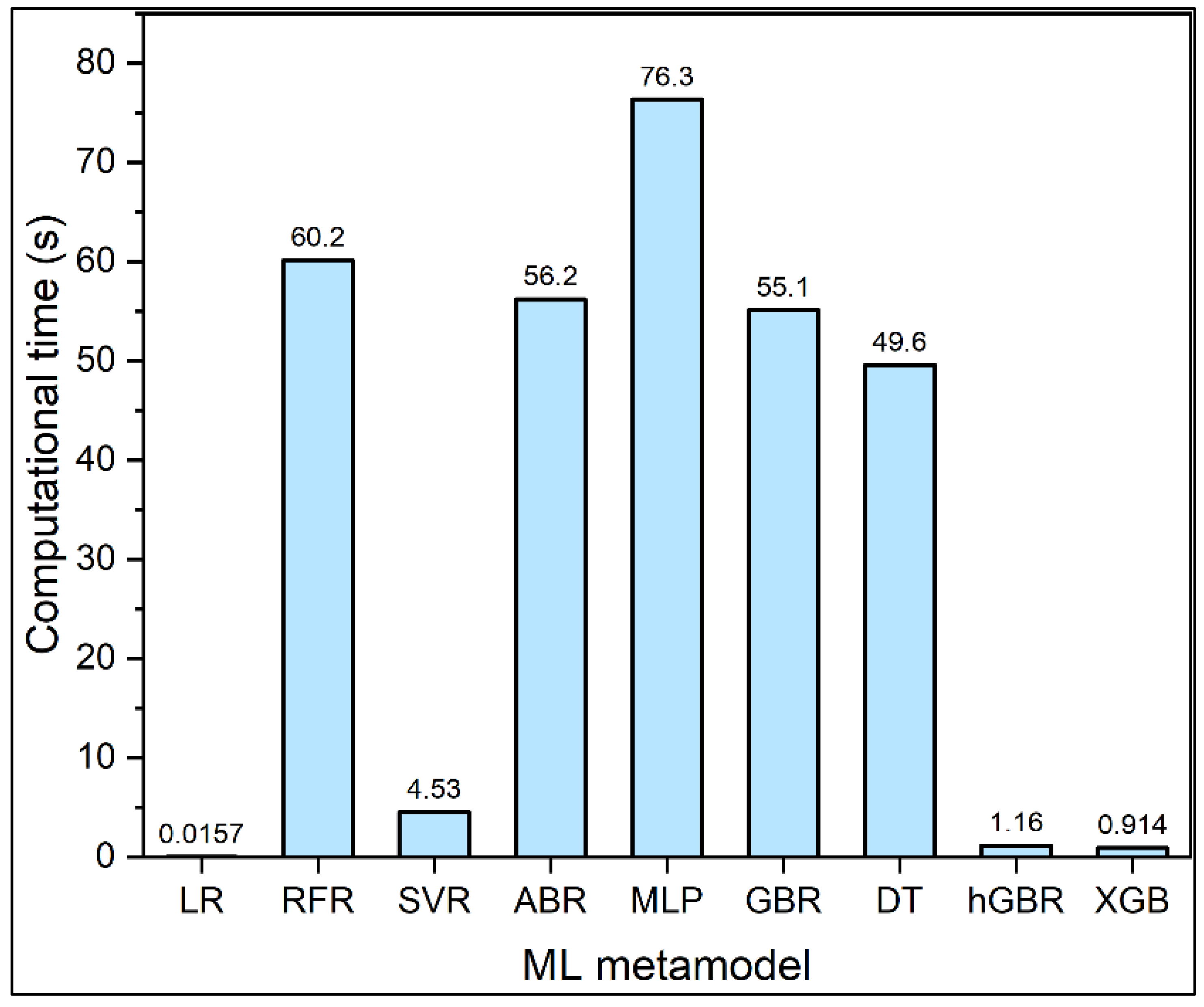
• In terms of computational time, the metamodels can be arranged from most expensive to least expensive as MLP > RFR > ABR > GBR > DT > SVR > hGBR > XGB > LR;
• Using a MADM method called TOPSIS, the metamodels can be ranked from best to worst based on a compromise solution as XGB > hGBR > SVR > GBR > DT > RFR > MLP > ABR > LR.

References

1. Pavlikova, M.; Brtník, T.; Keppert, M.; Černỳ, R. Effect of metakaolin as partial Portland-cement replacement on properties of high-performance mortars. Cem. Wapno Beton 2009, 3, 115–122. [Google Scholar]
2. Khatib, J.M.; Negim, E.M.; Gjonbalaj, E. High volume metakaolin as cement replacement in mortar. World J. Chem. 2012, 7, 7–10. [Google Scholar] [CrossRef]
3. Wianglor, K.; Sinthupinyo, S.; Piyaworapaiboon, M.; Chaipanich, A. Effect of alkali-activated metakaolin cement on compressive strength of mortars. Appl. Clay Sci. 2017, 141, 272–279. [Google Scholar] [CrossRef]
4. Yang, C.; Huang, R. A two-phase model for predicting the compressive strength of concrete. Cem. Concr. Res. 1996, 26, 1567–1577. [Google Scholar] [CrossRef]
5. Onal, O.; Ozturk, A.U. Artificial neural network application on microstructure-compressive strength relationship of cement mortar. Adv. Eng. Softw. 2010, 41, 165–169. [Google Scholar] [CrossRef]
6. Asteris, P.G.; Apostolopoulou, M.; Skentou, A.D.; Moropoulou, A. Application of artificial neural networks for the prediction of the compressive strength of cement-based mortars. Comput. Concr. 2019, 24, 329–345. [Google Scholar] [CrossRef]
7. Eskandari-Naddaf, H.; Kazemi, R. ANN prediction of cement mortar compressive strength, influence of cement strength class. Constr. Build. Mater. 2017, 138, 1–11. [Google Scholar] [CrossRef]
8. Sharifi, Y.; Hosseinpour, M. A predictive model-based ANN for compressive strength assessment of the mortars containing metakaolin. J. Soft Comput. Civ. Eng. 2020, 4, 1–12. [Google Scholar] [CrossRef]
9. Asteris, P.G.; Apostolopoulou, M.; Armaghani, D.J.; Cavaleri, L.; Chountalas, A.T.; Guney, D.; Hajihassani, M.; Hasanipanah, M.; Khandelwal, M.; Karamani, C.; et al. On the Metaheuristic Models for the Prediction of Cement-Metakaolin Mortars Compressive Strength; Techno-Press: Plovdiv, Bulgaria, 2020; Volume 1, p. 063. [Google Scholar] [CrossRef]
10. Ly, H.-B.; Nguyen, M.H.; Pham, B.T. Metaheuristic optimization of Levenberg–Marquardt-based artificial neural network using particle swarm optimization for prediction of foamed concrete compressive strength. Neural Comput. Appl. 2021, 33, 17331–17351. [Google Scholar] [CrossRef]
11. Zhao, Y.; Hu, H.; Song, C.; Wang, Z. Predicting compressive strength of manufactured-sand concrete using conventional and metaheuristic-tuned artificial neural network. Measurement 2022, 194, 110993. [Google Scholar] [CrossRef]
12. Sun, L.; Koopialipoor, M.; Armaghani, D.J.; Tarinejad, R.; Tahir, M.M. Applying a meta-heuristic algorithm to predict and optimize compressive strength of concrete samples. Eng. Comput. 2021, 37, 1133–1145. [Google Scholar] [CrossRef]
13. Armaghani, D.J.; Asteris, P.G. A comparative study of ANN and ANFIS models for the prediction of cement-based mortar materials compressive strength. Neural Comput. Appl. 2021, 33, 4501–4532. [Google Scholar] [CrossRef]
14. Sevim, U.K.; Bilgic, H.H.; Cansiz, O.F.; Ozturk, M.; Atis, C.D. Compressive strength prediction models for cementitious composites with fly ash using machine learning techniques. Constr. Build. Mater. 2021, 271, 121584. [Google Scholar] [CrossRef]
15. Asteris, P.G.; Cavaleri, L.; Ly, H.-B.; Pham, B.T. Surrogate models for the compressive strength mapping of cement mortar materials. Soft Comput. 2021, 25, 6347–6372. [Google Scholar] [CrossRef]
16. Dao, D.V.; Adeli, H.; Ly, H.-B.; Le, L.M.; Le, V.M.; Le, T.-T.; Pham, B.T. A Sensitivity and Robustness Analysis of GPR and ANN for High-Performance Concrete Compressive Strength Prediction Using a Monte Carlo Simulation. Sustainability 2020, 12, 830. [Google Scholar] [CrossRef] [Green Version]
17. Mohammed, A.; Rafiq, S.; Sihag, P.; Kurda, R.; Mahmood, W.; Ghafor, K.; Sarwar, W. ANN, M5P-tree and nonlinear regression approaches with statistical evaluations to predict the compressive strength of cement-based mortar modified with fly ash. J. Mater. Res. Technol. 2020, 9, 12416–12427. [Google Scholar] [CrossRef]
18. Abdalla, A.; Salih, A. Implementation of multi-expression programming (MEP), artificial neural network (ANN), and M5P-tree to forecast the compression strength cement-based mortar modified by calcium hydroxide at different mix proportions and curing ages. Innov. Infrastruct. Solut. 2022, 7, 153. [Google Scholar] [CrossRef]
19. Asteris, P.G.; Koopialipoor, M.; Armaghani, D.J.; Kotsonis, E.A.; Lourenço, P.B. Prediction of cement-based mortars compressive strength using machine learning techniques. Neural Comput. Appl. 2021, 33, 13089–13121. [Google Scholar] [CrossRef]
20. Çalışkan, A.; Demirhan, S.; Tekin, R. Comparison of different machine learning methods for estimating compressive strength of mortars. Constr. Build. Mater. 2022, 335, 127490. [Google Scholar] [CrossRef]
21. Ozcan, G.; Kocak, Y.; Gulbandilar, E. Estimation of compressive strength of BFS and WTRP blended cement mortars with machine learning models. Comput. Concr. 2017, 19, 275–282. [Google Scholar] [CrossRef]
22. Montgomery, D.C.; Peck, E.A.; Vining, G.G. Introduction to Linear Regression Analysis; John Wiley & Sons: Hoboken, NJ, USA, 2021. [Google Scholar]
23. Biau, G.; Scornet, E. A random forest guided tour. TEST 2016, 25, 197–227. [Google Scholar] [CrossRef] [Green Version]
24. Smola, J.; Schölkopf, B. A tutorial on support vector regression. Statistics and computing. Stat. Comput. 2004, 14, 199–222. [Google Scholar] [CrossRef] [Green Version]
25. Solomatine, D.P.; Shrestha, D.L. AdaBoost. RT: A boosting algorithm for regression problems. In Proceedings of the 2004 IEEE International Joint Conference on Neural Networks (IEEE Cat. No. 04CH37541), Budapest, Hungary, 25–29 July 2004. [Google Scholar]
26. Murtagh, F. Multilayer perceptrons for classification and regression. Neurocomputing 1991, 2, 183–197. [Google Scholar] [CrossRef]
27. Friedman, J.H. Stochastic gradient boosting. Comput. Stat. Data Anal. 2002, 38, 367–378. [Google Scholar] [CrossRef]
28. Myles, J.; Feudale, R.N.; Liu, Y.; Woody, N.A.; Brown, S.D. An introduction to decision tree modeling. J. Chemom. 2004, 18, 275–285. [Google Scholar] [CrossRef]
29. Chen, T.; Guestrin, C. Xgboost: A scalable tree boosting system. In Proceedings of the 22nd ACM SIGKDD International Conference on Knowledge Discovery and Data Mining, San Francisco, CA, USA, 13–17 August 2016. [Google Scholar]
30. Ashok, M.; Parande, A.K.; Jayabalan, P. Strength and durability study on cement mortar containing nano materials. Adv. Nano Res. 2017, 5, 99. [Google Scholar] [CrossRef]
31. Batis, G.; Pantazopoulou, P.; Tsivilis, S.; Badogiannis, E. The effect of metakaolin on the corrosion behavior of cement mortars. Cem. Concr. Compos. 2005, 27, 125–130. [Google Scholar] [CrossRef]
32. Courard, L.; Darimont, A.; Schouterden, M.; Ferauche, F.; Willem, X.; Degeimbre, R. Durability of mortars modified with metakaolin. Cem. Concr. Res. 2003, 33, 1473–1479. [Google Scholar] [CrossRef]
33. Curcio, F.; DeAngelis, B.; Pagliolico, S. Metakaolin as a pozzolanic microfiller for high-performance mortars. Cem. Concr. Res. 1998, 28, 803–809. [Google Scholar] [CrossRef]
34. Cyr, M.; Idir, R.; Escadeillas, G.; Julien, A.N.M.S. Stabilization of Industrial By-Products in Mortars Containing Metakaolin; ACI Special Publication, (242 SP); American Concrete Institute: Farmington Hills, MI, USA, 2007; pp. 51–62. [Google Scholar] [CrossRef]
35. D’Ayala, D.; Fodde, E. Blended lime-cement mortars for conservation purposes: Microstructure and strength development. In Structural Analysis of Historic Construction: Preserving Safety and Significance; Two Volume Set; CRC Press: Boca Raton, FL, USA, 2008; pp. 1005–1012. [Google Scholar]
36. Geng, H.N.; Li, Q. Water Absorption and Hydration Products of Metakaolin Modified Mortar. Key Eng. Mater. 2017, 726, 505–509. [Google Scholar] [CrossRef]
37. Al-Chaar, G.; Alkadi, M.; Asteris, P.G. Natural Pozzolan as a Partial Substitute for Cement in Concrete. Open Constr. Build. Technol. J. 2013, 7, 33–42. [Google Scholar] [CrossRef] [Green Version]
38. Kadri, E.-H.; Kenai, S.; Ezziane, K.; Siddique, R.; De Schutter, G. Influence of metakaolin and silica fume on the heat of hydration and compressive strength development of mortar. Appl. Clay Sci. 2011, 53, 704–708. [Google Scholar] [CrossRef]
39. Khater, H.M. Influence of Metakaolin on Resistivity of Cement Mortar to Magnesium Chloride Solution. J. Mater. Civ. Eng. 2011, 23, 1295–1301. [Google Scholar] [CrossRef]
40. Khatib, J.; Wild, S. Sulphate Resistance of Metakaolin Mortar. Cem. Concr. Res. 1998, 28, 83–92. [Google Scholar] [CrossRef]
41. Lee, S.; Moon, H.; Hooton, R.D.; Kim, J. Effect of solution concentrations and replacement levels of metakaolin on the resistance of mortars exposed to magnesium sulfate solutions. Cem. Concr. Res. 2005, 35, 1314–1323. [Google Scholar] [CrossRef]
42. Mansour, M.S.; Abaldia, T.; Jauberthie, R.; Messaoudenne, I. Metakaolin as a pozzolan for high performance mortar. Cem. Wapno Beton 2012, 2, 102–108. [Google Scholar]
43. Mardani-Aghabaglou, A.; Sezer, G.İ.; Ramyar, K. Comparison of fly ash, silica fume and metakaolin from mechanical properties and durability performance of mortar mixtures view point. Constr. Build. Mater. 2014, 70, 17–25. [Google Scholar] [CrossRef]
44. Sumasree, C.; Sajja, S. Effect of metakaolin and cerafibermix on mechanical and durability properties of mortars. Int. J. Sci. Eng. Technol. 2016, 4, 501–506. [Google Scholar]
45. Vu, D.; Stroeven, P.; Bui, V. Strength and durability aspects of calcined kaolin-blended Portland cement mortar and concrete. Cem. Concr. Compos. 2001, 23, 471–478. [Google Scholar] [CrossRef]
46. Parande, A.K.; Babu, B.R.; Karthik, M.A.; Kumaar, K.D.; Palaniswamy, N. Study on strength and corrosion performance for steel embedded in metakaolin blended concrete/mortar. Constr. Build. Mater. 2008, 22, 127–134. [Google Scholar] [CrossRef]
47. Potgieter-Vermaak, S.S.; Potgieter, J.H. Metakaolin as an extender in South African cement. J. Mater. Civ. Eng. 2006, 18, 619–623. [Google Scholar] [CrossRef]
48. Saidat, F.; Mouret, M.; Cyr, M. Chemical Activation of Metakaolin in Cement-Based Materials. Spec. Publ. 2012, 288, 1–15. [Google Scholar] [CrossRef]
49. Kalita, K.; Pal, S.; Haldar, S.; Chakraborty, S. A Hybrid TOPSIS-PR-GWO Approach for Multi-objective Process Parameter Optimization. Process Integr. Optim. Sustain. 2022, 1–16. [Google Scholar] [CrossRef]
50. Shinde, D.; Öktem, H.; Kalita, K.; Chakraborty, S.; Gao, X.-Z. Optimization of Process Parameters for Friction Materials Using Multi-Criteria Decision Making: A Comparative Analysis. Processes 2021, 9, 1570. [Google Scholar] [CrossRef]
Figure 1. Pair plots for the input parameters and observed responses.
Processes 10 01387 g001
Figure 2. Correlation heatmap of input parameters and observed responses.
Processes 10 01387 g002
Figure 3. Effect of number of estimators on random forest regression’s performance in terms of (a) MAE, (b) MSE and (c) R 2 .
Processes 10 01387 g003
Figure 4. Effect of number of estimators on AdaBoost regression’s performance in terms of (a) MAE, (b) MSE and (c) R 2 .
Processes 10 01387 g004
Figure 5. Effect of number of perceptrons on MLP’s performance in terms of (a) MAE, (b) MSE and (c) R 2 .
Processes 10 01387 g005
Figure 6. Effect of number of estimators on gradient boosting regression’s performance in terms of (a) MAE, (b) MSE and (c) R 2 .
Processes 10 01387 g006
Figure 7. Actual versus predicted compressive strength of cement-based mortars using (a) linear regression, (b) random forest regression, (c) support vector regression, (d) AdaBoost regression, (e) multi-layer perceptron and (f) gradient boosting regression. Actual versus predicted compressive strength of cement-based mortars using (g) decision tree regression, (h) hist gradient boosting regression and (i) XGBoost regression.
Processes 10 01387 g007aProcesses 10 01387 g007b
Figure 8. Computational time of each ML metamodel.
Processes 10 01387 g008
Figure 9. Distance of each alternative (ML metamodel) from the hypothetical ideal solution.
Processes 10 01387 g009