A Comparative Study of Indoor Accuracies Between SLAM and Static Scanners

Abstract

This study presents a comprehensive comparison of static and SLAM (Simultaneous Localization and Mapping) laser scanners of both new and old generation in a controlled indoor environment of a standard commercial building with long, linear corridors and recesses. The aim was to assess both global and local accuracy, as well as noise characteristics, of each scanner. Methods: A highly accurate static scanner was used to generate a reference point cloud. Five devices were evaluated: two static scanners (Leica RTC 360 and Trimble X7) and three SLAM scanners (GeoSLAM ZEB Horizon RT, Emesent Hovermap ST-X, and FARO Orbis). Accuracy analysis included systematic and random error assessment, axis-specific displacement evaluation, and profile-based local accuracy measurements. Additionally, noise was quantified before and after data smoothing. Static scanners yielded superior accuracies, with the Leica RTC 360 achieving the best performance (absolute accuracy of 1.2 mm). Among SLAM systems, the Emesent Hovermap ST-X and FARO Orbis—both newer-generation devices—demonstrated significant improvements over the older-generation GeoSLAM ZEB Horizon RT. After smoothing, the noise levels of these new-generation SLAM scanners (approx. 2.1–2.2 mm) approached those of static systems. The findings underline the ongoing technological progress in SLAM systems, with the new-generation SLAM scanners becoming increasingly viable alternatives to static scanners, especially when speed, ease of use, and reduced occlusions are prioritized. This makes them well-suited for rapid indoor mapping applications, provided that the slightly lower accuracy is acceptable for the intended use.

1. Introduction

3D scanning is increasingly coming to the forefront of the focus of designers, contractors, and surveyors. This is especially true with the development of SLAM (Simultaneous Localization and Mapping) technology that enables rapid data collection and, thus, allows capturing the actual state of the construction processes (even retrospectively, if needed), thereby improving quality control. Data acquired in this way can be also easily used for the documentation of building information management/modeling (BIM).

So far, static scanners with accuracies of several millimeters [1] have been used for measurements even in applications where only centimeter-level accuracies were needed. More recently, mobile scanners mounted on cars or similar vehicles have been used for this purpose in the case of linear constructions [2]. Additionally, lidar-based scanners mounted on unmanned aerial vehicles (UAVs) have also found their place in surveying [3,4].

Scanning speeds range from hundreds of thousands to millions of points per second. Laser scanning is quite sufficient for capturing the space in many applications, such as studies on earthquake-induced landscape changes [5], digital terrain model creation [6], geohazard areas mapping [7], trees and forests [8,9], agriculture [10], vegetation structure [11], underground structures [12], emergency vehicles passage planning [13], and even the evaluation of the avalanche hazard in steep snow-covered areas [14]. Where constructions are concerned, laser scanning is mostly used for the purposes of BIM [15], evaluation of the road condition [16], creating digital twins of bridges [17] or towers [18], and the documentation of various peculiar construction shapes, such as astronomical domes [19].

For building interiors, laser scanning methods are increasingly used as the principal surveying method allowing the creation of real-state documentation. Compared to (for example) underground spaces, such as mines or caves, the digitization of the acquired data is usually simple in buildings as it typically involves predominantly planar objects (walls, ceilings, floors) with few obstructions. The practical acquisition of a digital twin of a building interior using static scanners, which are characterized by high accuracy and low noise, is limited by the need to perform a scan separately in each room. This is significantly more time-consuming than in the case of SLAM scanners, allowing data acquisition during a simple passage through the object.

In static scanners, the overall accuracy consists of the accuracy of the scanner sensor and of scanner positioning, which is typically determined either as a spatial intersection from ground control points or through the Iterative Closest Point algorithm applied to the point cloud). The assessment of SLAM scanners’ accuracies is usually a more complex task as, besides the accuracy of the sensor itself, establishing the trajectory of the scanner also plays a crucial role. Determining the trajectory is, therefore, a complex process that is largely dependent on the quality of the software that comes with the scanner. Establishing the achievable accuracy of the resulting data in advance is, therefore, more complicated than in the case of static scanners. Besides the difficult determination of the accuracy in SLAM scanners, their results can be also expected to yield higher noise than static scanners [20]; the use of suitable processing methods can, however, greatly improve the final result [21].

SLAM scanners are nowadays used for many purposes previously reserved for static scanners; this is especially true in building interiors, where this technology offers great promise [22]. Importantly, new SLAM algorithms and systems, including hardware [23] are still being developed and the whole SLAM technology is moving forward rapidly. A generational change is currently underway, with more accurate SLAM sensors coming to the market. According to their manufacturers‘ declarations of accuracies and reliabilities, such scanners should be already suitable for surveyor work, being (at least in some parameters) on par with the terrestrial static systems. These improvements can be seen, for example, in the increased number of channels registered by the scanning head from 16 to 32 or in the improved accuracy of distance determination. Although the evaluation of the suitability and accuracy of SLAM scanners has been discussed in several studies [24,25,26], detailed testing and comparison of multiple scanners of older and newer generations under real interior conditions is, however, not available so far.

This study aims to evaluate (in particular) the accuracy of multiple SLAM scanning systems available on the market in a representative building interior (a technical floor of an administrative building) and to compare the results of the newer and older SLAM scanners using reference data obtained with a high-accuracy static scanner.

2. Materials and Methods

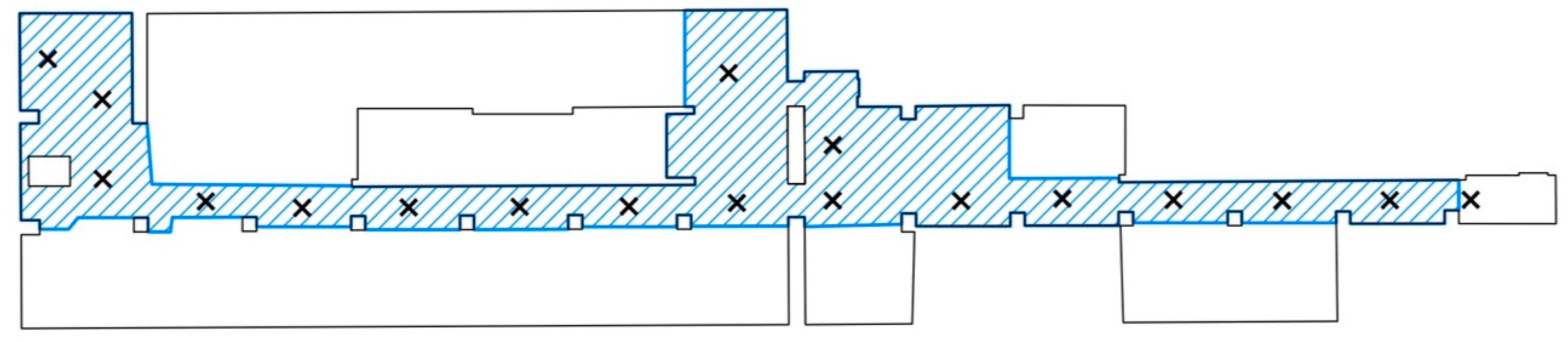
To address the aforementioned aims, an experiment comparing the quality of point clouds acquired with static scanners, old- and new-generation SLAM scanners were devised in an environment suitable for the use of these scanners. An interior building environment with a relatively long, straight corridor with recesses allowing us to analyze the accumulation of systematic and random errors when using SLAM scanners was selected for this study. All analyses of SLAM scanner accuracy were performed against a reference dataset obtained using an accurate static scanner Leica ScanStation P40 (Leica Geosystems AG, Heerbrugg, Switzerland) combined with a highly accurate geodetic network established with the Trimble S9 HP total station (Trimble Inc., Westminster, CO, USA).

2.1. Testing Space

The scanners were tested on the technical floor of Building B, Faculty of Civil Engineering of the Czech Technical University. The schematic layout of its shape and the used geodetic network are shown in Figure 1a, with photos of its central part shown in Figure 1b,c. The accurate geodetic network was stabilized using reflective targets (Figure 1d) and georeferenced with the Trimble S9 HP total station with a subsequent least squares alignment.

To establish the reference geodetic network using the Leica ScanStation P40 scanner, special black and white targets (6001 to 6018) were placed throughout the study area (Figure 2a). Some targets were made of paper and placed on the walls (stabilized with paper tape), while others (plastic) were stabilized using magnetic bases (Figure 2b,c). In addition, spherical targets with a radius of 7 cm (5001 to 5006) were installed for the purpose of georeferencing the clouds of the tested scanners. A layout of their placement is shown in Figure 2d. They were stabilized using a metal platform with two nuts attached to the wall with a high-strength adhesive. The spherical targets (containing a magnetic element) were attached to the platform so that they were resting on the two nuts, and two lines connecting the plate and the magnetic element were drawn with a permanent marker to ensure consistent and repeatable positioning; see Figure 2e.

2.2. Used Instruments

A Trimble S9 HP robotic total station (Figure 3a) with a standard deviation of distance measurement of 0.8 mm + 1.0 ppm on a prism (2 mm + 2 ppm on an arbitrary surface) and the standard deviation of the horizontal direction and zenith angle measurement of 0.3 mgon was used for the absolute georeferencing of the coordinate network using the reflective targets as well as for the determination of the centers of the black and white paper targets.

A Leica ScanStation P40 terrestrial scanner (Figure 3b) with a field of view of 360° × 270°, distance measurement accuracy of 1.2 mm + 10 ppm, angular accuracy of 8”, liquid compensator with an accuracy of 1.5”, maximum measurement distance of 270 m (considering 18% reflectance), and scanning speed of 1 million points per s was used for terrestrial laser scanning. Black and white targets were used for georeferencing of the point clouds acquired from the individual positions.

Five scanners were evaluated: two static scanners Trimble X7 (Trimble Inc., Westminster, CO, USA) and Leica RTC 360 (Leica Geosystems AG, Heerbrugg, Switzerland) and three SLAM scanners (GeoSLAM ZEB Horizon RT (Faro, Lake Mary, FL, USA), Emesent Hovermap ST-X (Emesent Pty Ltd., Milton, Queensland, Australia), and FARO Orbis (Faro, Lake Mary, FL, USA)).

The first of the tested scanners, Leica RTC 360 (Figure 3c), offers three scanning resolution options (3/6/12 mm at 10 m), determination of the scanner position through real-time tracking of movement using a VIS unit, and automatic filtering of moving objects. The scanner range is 130 m. An Apple tablet with a Leica Cyclone FIELD 360 app was used for the measurement.

Trimble X7 (Figure 3d) is a static scanner characterized by its focus on measurement speed. ICP transformation is the primary method of registering clouds, with the option of manual targeting of the centers of targets serving as (ground) control points. The instrument features self-leveling within 10° and can take measurements even when upside down. An automatic calibration (approx. 20 s) was performed before triggering the measurement. Trimble X7 uses a wavelength of 1550 nm (invisible, Class 1 laser according to [27] for the measurement. It also features a field of view of 360° (horizontal) × 282° (vertical), a range of 0.6 m to 80 m, a manufacturer-declared standard deviation of distance measurement accuracy of 2 mm and angular measurement accuracy of 21”. The measurement speed is up to 500,000 pts/s. It has three calibrated cameras, 10 Mpix each, acquiring up to 316 Mpix of image data per station. It is controlled via a Wi-Fi-connected Trimble T10 tablet (Trimble Inc., Westminster, CO, USA) with Trimble Perspective software ver. 2024.00. Its dimensions are 353 mm × 178 mm × 170 mm, and its weight is 5.8 kg (including battery). Data is stored on an SD card and was continuously transferred to the control tablet.

The lidar range of the Emesent Hovermap ST-X (Figure 3e) is 0.5–300 m, with a declared distance accuracy of 10 mm. The scanner has 32 (lidar) channels, scanning speed of 640,000/s considering a single return (up to three returns can be registered). It can store up to 512 GB of data (approx. 4 h of scanning). At its weight of 1.57 kg, it can be carried by an individual as a handheld scanner, mounted on a backpack, a vehicle, or a robot. The distributor claims a mapping accuracy of 15 mm under general conditions, 10 mm in indoor environment, and a local accuracy standard deviation of 5 mm. Data was processed in a proprietary Emesent Aura software ver. 1.8.1.

The GeoSLAM ZEB Horizon RT (Figure 3f), paired with the GeoSLAM Connect 2.3.0 processing software, has a maximum range of 100 m and a field of view of 360° × 270°. The weight of the scanner is 1.45 kg and that of the data logger including the battery is 1.4 kg. The scanner is based on the Velodyne VLP-16 sensor (Velodyne Lidar, San Jose, CA, USA), capable of scanning 300,000 points per second via 16 rangefinders (called “channels” in the manufacturer-provided information), the claimed relative accuracy is up to 6 mm. The GeoSLAM Accuracy Report also claims that 95% of the points in the cloud are within ±19 mm of the correct (reference) cloud targeted by a more accurate method.

The Faro Orbis (Figure 3g) scanner features a maximum range of 120 m, scanning speed of 640,000 points/s, and field of view of 290° × 360°. The scanner has 32 lidar channels, a 360° 8 Mpix camera (once per second), measurement accuracy (SD) of 5 mm, and a Class 1 laser. The scanner weighs 2.1 kg, with an additional data logger weight of 0.95 kg. The FARO Stream app (for iOS and Android) provides scanner control, real-time data visualization, and direct sync to cloud processing with FARO Sphere XG (Faro, Lake Mary, FL, USA). The internal storage capacity is 1 TB (up to 100 h of continuous data capture). It can also perform a so-called static scan, with 19 million points acquired over 15 s, with an Improved accuracy of 2 mm. The device is also capable of identifying reference points from the cloud and using them to adjust the scanning trajectory. Moreover, placing the scanner on a georeferenced point during a pass is automatically taken into account for improving the trajectory reconstruction.

Measurements with instruments in our possession (Leica ScanStation P40, Trimble X7, Trimble S9 HP) and associated data processing were performed by the authors. The basic processing of point clouds from Leica ScanStation P40 was performed in Leica Cyclone software v. 2023.0.1; the Trimble X7 point cloud was processed using the Trimble T10 tablet with Trimble Perspective software ver 2024.00 (which can be also installed on a suitable Windows 11 computer). The GNU Gama software v. 2.33 was used for data acquired from the total station.

For the remaining instruments, the measurement and primary data processing were performed by the employees of the official distributors of the respective instruments within the Czech Republic. Data processing was performed in the proprietary software solutions for each of the scanners in versions valid by February 2024.

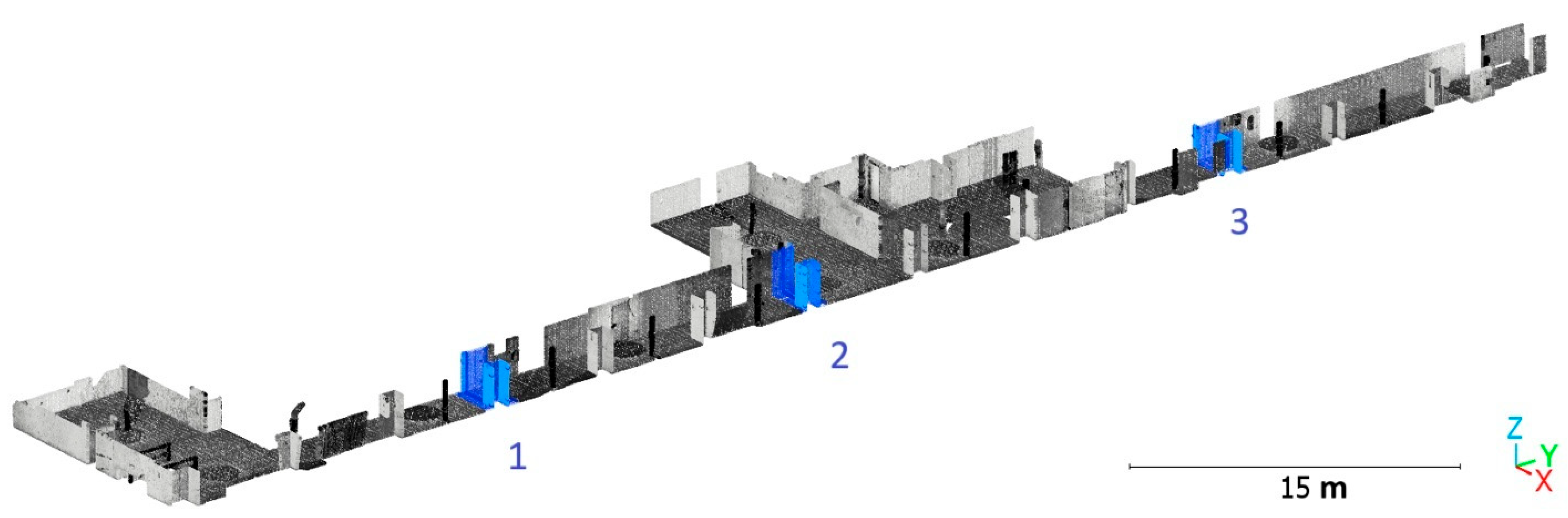
2.3. Reference Cloud Acquisition

Prior to scanning, both spherical and black and white targets were placed within the area and georeferenced using the total station. Subsequently, scanning with the Leica ScanStation P40 with settings of point density of 3.1 mm per 10 m, normal sensitivity, and full field of view was carried out from 11 stations. The measurement from each station took approximately 3.5 min. After scanning from each station, reference points for Leica P40 (black and white targets; Figure 2) were identified in the cloud using a built-in feature (the targets were scanned with an improved density and their centers automatically detected). To verify the accuracy of the reference cloud, 58 control points on the walls and floor were georeferenced using the total station (from five positions). The root mean square error (RMSE) was calculated in CloudCompare using the Cloud-to-Cloud function (comparing the 58 points to the reference P40 cloud).

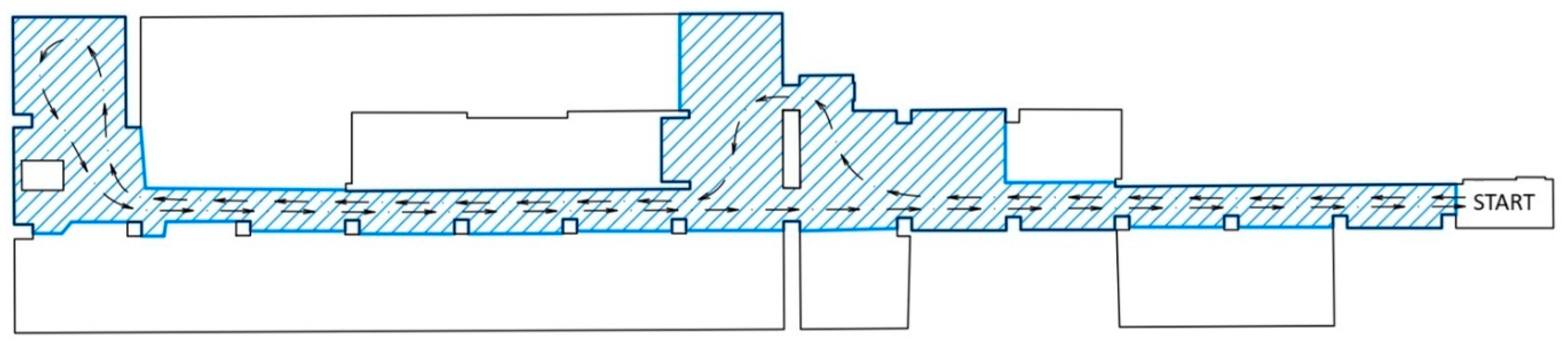
2.4. Measurements with the Tested Scanners

Due to the time-consuming nature of this measurement, measurements using static scanners were performed only once with each scanner. The approximate locations of individual scanning stations are shown in Figure 4.

The measurements with the Trimble X7 static scanner were carried out with a scanning time of two minutes, scanning option Standard, and a point density of 11 mm per 10 m. In view of the large number of stations (22) and the small distances between them, this point density was sufficient. The scanned clouds were automatically registered to each other during the measurements thanks to the sufficient overlap. The final registration was performed automatically during export in the Trimble Perspective software ver. 2024.00, with a mean error 1.3 mm as reported by the software.

Measurements with the Leica RTC 360 scanner were taken from a total of 19 sites with the minimum point density set to 12 mm at 10 m. The net scanning time was 26 s per station (image acquisition and moving object filtering were disabled). During the measurements, the data were automatically synchronized with an iOS tablet and the Leica Cyclone FIELD 360 app, where the data were manually checked and overlap registration was performed. The final registration was performed in the Cyclone REGISTER 360 PLUS software ver. 2024.0.2.

Thanks to the rapid scanning using SLAM scanners, measurement with each scanner was performed three times to also allow the evaluation of the consistency between passes. A schematic of individual measurement passes is shown in Figure 5.

Measurements with the Emesent Hovermap ST-X scanner were performed in manual mode after initialization of 10 s, with a single back-and-forth-pass taking less than 4 min. Data registration was performed in the Aura software ver. 1.8.1.

Similarly, the measurements with GeoSLAM ZEB Horizon RT and FARO Orbis were performed after a 10 s initialization (in a stationary position on a solid base) for approx. 10 s, each scanning pass took approx. 4.5 min.

2.5. Principles of the Evaluation of the Individual Clouds

Each measurement contains both systematic and random errors. By the term “systematic error”, we will refer to the principal component of the systematic error, i.e., bending of the cloud (the “banana-shaped error”) in this paper. This error can result from the misregistration of the clouds on the overlap from multiple stations (in terrestrial scanners) or from the incorrect determination of the trajectory (during SLAM scanning). The random error, on the other hand, is more uniformly distributed throughout the entire cloud. Both types of error are illustrated in Figure 6, showing the two types of error arising in a cloud georeferenced to spherical targets placed at both ends of the cloud. Iterative closest point transformation will lead to an improvement of the systematic error by about 50% (see the dotted line in Figure 6).

2.6. Processing and Evaluation of the Acquired Data

2.6.1. Initial Processing

This experiment was devised to mimic the everyday practical use of the scanners. Before the evaluation, the point clouds were cleaned of undesirable points (scanned moving persons, obvious noise, etc.).

As any point cloud represents a complex representation of the scanned space, multiple characteristics were used for the evaluation of the results. Regardless of the type of scanner, further processing of the primary clouds acquired from the proprietary software was performed in CloudCompare v. 2.12.

First, the clouds acquired using the static scanners were diluted. The reference cloud was diluted to a density of 4 mm to maintain high surface detail. Clouds from the tested static scanners were diluted to 1 cm to even out the density (there were places with excessive density, especially in the vicinity of the scanning stations). No point cloud reduction was performed in the SLAM scanners due to the character of the distribution of the points—in view of the high noise, such dilution would predominantly remove points from the most dense (most accurate) part of the distribution.

Further evaluation utilized root mean square error (RMSE) as a metric and served to compare (i) the whole clouds and (ii) specific sections of the cloud to obtain further information.

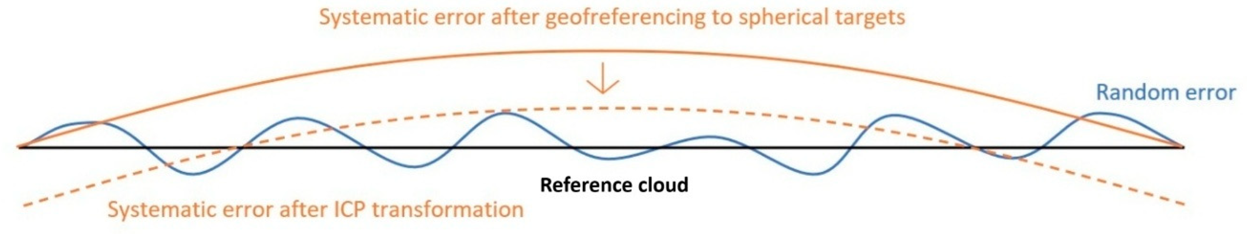
2.6.2. Transformation of the Clouds to Spherical Targets

In general, point clouds from the tested scanning systems were georeferenced using the spatial transformation (scale = 1) to the local reference cloud coordinate system based on the spherical targets (only targets No. 5001, 5002, 5005, and 5006 located at the extreme ends of the trajectory were used to allow subsequent determination of the errors arising along the route). The clouds were transformed using the function Align two clouds by picking (at least 4) equivalent point pairs. Subsequently, each cloud was cropped to contain only the area captured by the reference scanner. Ideally, the cloud transformed in this way should be identical to the reference cloud.

Prior to the dilution, spherical targets serving as reference points were always carefully cut out, their centers determined and used to acquire transformation parameters (three angles of rotation along the X, Y, and Z axes and three displacements in the directions of the X, Y, and Z axes). Using these parameters, the cloud was transformed into the reference cloud system. The root mean square error of the initial transformation to the spherical targets (i.e., the distance between the centers of the spherical targets of the tested and reference cloud acquired after this basic transformation to spherical targets—RMSE_SPHER; Equation (1)) served as the first metric used to evaluate the scanner performance.

$${\mathrm{R}\mathrm{M}\mathrm{S}\mathrm{E}}_{\mathrm{S}\mathrm{P}\mathrm{H}\mathrm{E}\mathrm{R}}=\sqrt{{\displaystyle \frac{\sum _1^{\mathrm{n}}{\mathrm{d}}_{\mathrm{i}}^2}{\mathrm{n}}}}$$

(1)

where d is the distance describing the difference between the reference points (the centers of the four spherical targets) of the tested and reference cloud and n is the number of these distances (in this case, n = 4).

This parameter reflects, in particular, the error in the distance between the initial and furthest points of the trajectory. To a smaller degree, it also reflects the quality of the determination of the centers of the spherical targets in the cloud. It is important to point out that the shape of the cloud is not altered during this or any other transformation used in this paper—only displacements and rotations of the entire cloud are applied here.

2.6.3. The Overall Accuracy of Individual Clouds After the Initial Transformation

The overall root mean square error between the test and the reference clouds (RMSE_OVERALL) was determined as follows: For each point of the test cloud, an irregular triangular area network (TIN) was constructed from the 15 nearest points of the reference cloud, and the distance of the point relative to this TIN surface was determined.

2.6.4. ICP Transformation and Evaluation of the Transformed Clouds

For better evaluation of the shape of the individual clouds (i.e., systematic error, see Figure 6), the iterative closest point (ICP) transformation of the entire test cloud to the reference cloud was performed. For this step, the Fine registration (ICP) function in CloudCompare was used. The Random sampling limit was increased to make sure that the entire cloud was used for the transformation and the filtering of the outliers (most distant points) was enabled. Again, we emphasize that the shape of the cloud was not changed, transformation was based solely on displacements and rotations of the entire clouds.

Next, RMSE_ICP-ALL (i.e., the RMSE of the entire cloud after ICP transformation) was calculated. In this way, the effect of the transformation to spherical targets was eliminated and (as shown in Figure 6), the RMSE was expected to drop by about 50%. This parameter, therefore, allows a qualitative assessment of the shape of the test cloud compared to the reference (note that this evaluation cannot be performed in the practical real-world setting where the reference cloud is not available).

2.6.5. Local ICP Transformation for Evaluation of Profiles

If the basic transformation to the spherical targets is used, the highest accuracies can be expected at the beginning and end of the trajectory (the clouds were georeferenced using points placed at the extreme ends of the floor) and the worst accuracy in the middle of the route. Therefore, continuous profiles located in approx. 25%, 50%, and 75% along the route were selected to evaluate the local accuracy of the individual clouds (see Figure 7, highlighted in blue).

Subsequently, we performed an additional local ICP transformation of the profiles (ICP-local) to the reference cloud (this allowed us to determine the displacement between the profile points transformed to accurately fit the reference cloud and the profile points after the overall transformation).

The ICP transformation procedure for individual profiles was identical to that for the whole cloud. Here, we aimed to determine the local characteristic displacements in individual axes (i.e., the values of the displacements in individual coordinate axes from the transformation matrix). For the purpose of the evaluation, values ∆X, ∆Y, ∆Z were calculated as root mean square error of displacements in individual axes from all profiles (i.e., 3 profiles × 3 passages for SLAM scanners and 3 profiles × 1 measurement for static scanners).

Lastly, the locally ICP-transformed profiles were compared with the reference profiles using the cloud/cloud distance function, yielding the RMSE_ICP-PROFILE value characterizing the local cloud accuracy.

2.6.6. Noise Evaluation

To determine the amount of noise, the test profiles were smoothed employing the Smooth using MLS function, using a radius of 0.05 m, a polynomial degree of 2, and a Gaussian quadratic parameter of 0.0025 m. The RMSE was then determined using the Compute stat params function with the Gaussian distribution option.

Removing the noise yielded a smooth cloud, representing the measured object more clearly. At the same time, however, it also introduced minor edge rounding, which slightly affected the resulting accuracy (had the search radius been smaller, the cloud would not be smoothed sufficiently; had it been larger, the edge rounding would be excessive).

The RMSE of the noise was calculated as the square root of the difference of the RMSE values obtained from individual profiles (and passes) before and after smoothing according to the formula:

$${RMSE}_{noise}=\sqrt{{RMSE}_{ICP-local}^2-{RMSE}_{ICP-local smoothed}^2}$$

(2)

To be able to compare the overall performance of the scanners, mean respective RMSEs (e.g., RMSE_SPHER-∅) were calculated from RMSEs acquired from the three individual passes using the formula

$${\mathrm{R}\mathrm{M}\mathrm{S}\mathrm{E}}_{\mathrm{\varnothing }}=\sqrt{{\displaystyle \frac{\left({\mathrm{R}\mathrm{M}\mathrm{S}\mathrm{E}}_1^2+{\mathrm{R}\mathrm{M}\mathrm{S}\mathrm{E}}_2^2+\dots +{\mathrm{R}\mathrm{M}\mathrm{S}\mathrm{E}}_{\mathrm{n}}^2\right)}{\mathrm{n}}}}$$

(3)

where n is the number of values.

3. Results

The accuracy of the reference cloud registration was characterized by a mean absolute error of 1.3 mm (based on internal scanner validation). Subsequently, the accuracy of the reference cloud was independently verified using 58 control points that were placed on the walls and floor and measured with a total station, yielding a RMSE of 1.4 mm. Given the expected accuracy of the SLAM scanners of approximately 1 cm, the reference point cloud is an order of magnitude more accurate and, therefore, suitable for use as a reference.

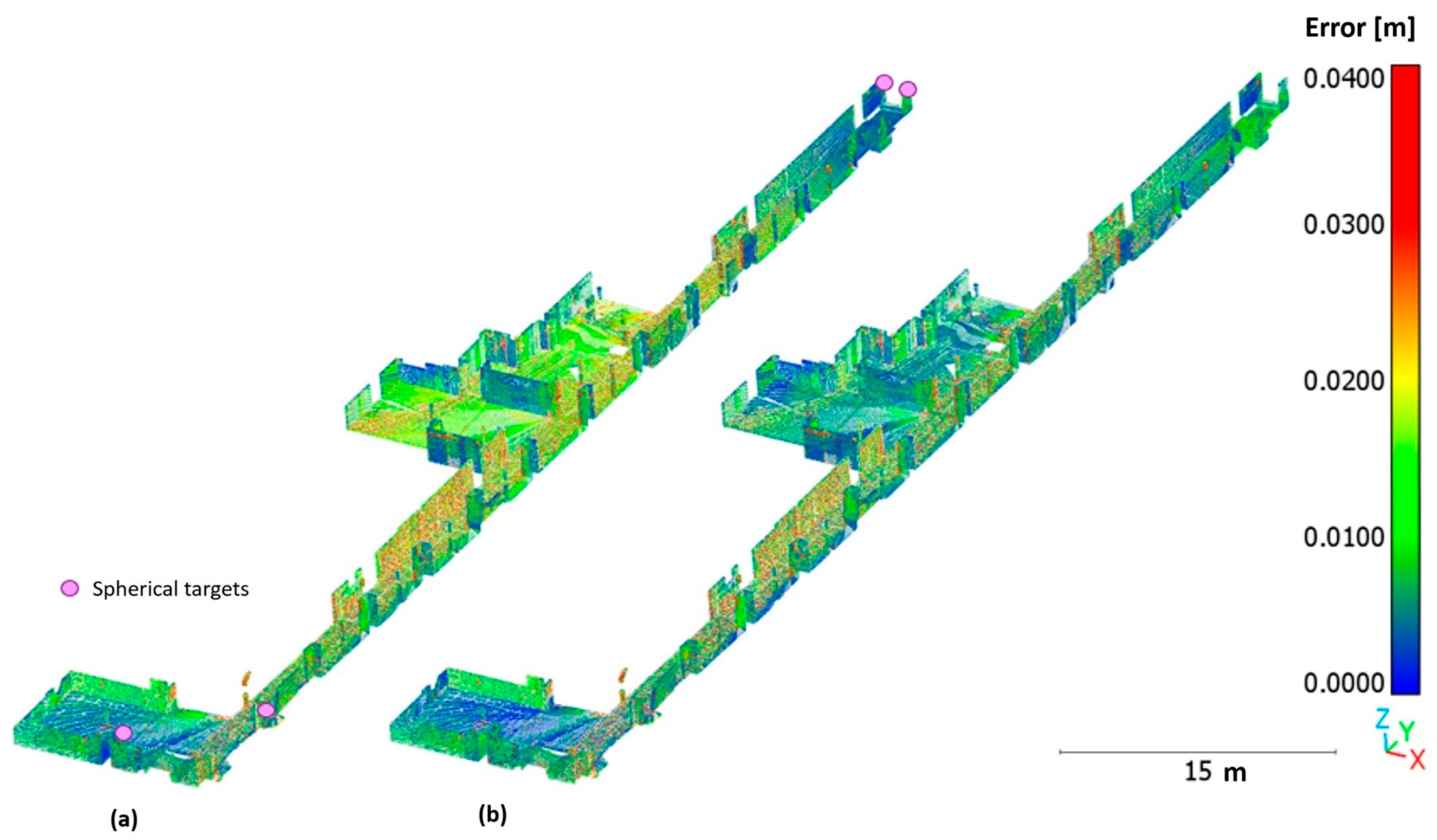
3.1. Initial Transformation to Spherical Targets

The parameter RMSE_SPHER describes the error of the cloud shape and dimensions after transformation (see Section 2.6.2) based on the four spherical targets (i.e., based solely on the four centers of the targets as described in Section 2.6.2). The results are presented in

Table 1. RMSE_SPHER values after initial transformation based on the four spherical targets used for georeferencing of the clouds and standard deviation (StDev in the brackets).

Scanner	Trimble X7	Leica RTC 360	Emesent Hovermap ST-X	GeoSLAM ZEB Horizon RT	FARO Orbis
RMSESPHER [mm] for individual measurements	2.0	1.5	4.4/5.5/4.8	17.5/15.9/17.9	6.6/8.0/3.9
RMSESPHERÆ [mm] (StDev)	2.0	1.5	4.9 (0.6)	17.1 (1.1)	6.4 (2.1)

. The lowest RMSE_SPHER was achieved by the static scanner Leica RTC 360, while the highest values were observed for the GeoSLAM ZEB Horizon RT.

3.2. Visual Quality of the Point Clouds

The visual quality of the point clouds will be presented on the appearance of the spherical targets scanned by individual scanners (Figure 8), including the result of the reference scanner Leica ScanStation P40 (Figure 8f). It clearly shows the low level of noise produced by static scanners (Trimble X7, Leica RTC 360—Figure 8a,b), with the cloud acquired with the Leica RTC 360 being smoother than Trimble X7. On the other hand, the high level of noise produced by SLAM scanners is also clearly visible, although the noise level of the newer ones (Emesent Hovermap ST-X, Figure 8c, and FARO Orbis, Figure 8e) is lower than that of the older generation SLAM scanner (GeoSLAM ZEB Horizon RT, Figure 8d). Even this simple visual comparison clearly demonstrates the technological advancement in the performance of newer SLAM scanners.

3.3. Accuracies of Clouds Transformed to Spherical Targets

The accuracies of entire point clouds acquired after the initial transformation to the four spherical targets (see Section 2.6.3) are presented in

Table 2. Absolute accuracies of individual clouds relative to the reference cloud (after initial transformation to spherical targets) and standard deviation (StDev in the brackets).

Scanner	Trimble X7	Leica RTC 360	Emesent Hovermap ST-X	GeoSLAM ZEB Horizon RT	FARO Orbis
RMSESPHER [mm] for individual measurements	5.4	1.2	5.9/6.6/9.1	31.5/35.3/41.2	9.0/8.2/9.3
RMSESPHERÆ [mm] (StDev)	5.4	1.2	7.3 (1.7)	36.2 (4.9)	8.8 (0.6)

. The Leica RTC 360 performed the best (RMSE of 1.2 mm), while the worst performance was detected for the old-generation SLAM scanner ZEB Horizon (36.2 mm).

3.4. Global Point Cloud Accuracies After Icp Transformation

The RMSE_ICP-ALL better characterizes the systematic error (bending) of the individual clouds, see Chapter 2.6.4 (

Table 3. Relative accuracies of individual clouds (after ICP transformation) and standard deviation (StDev in the brackets).

Scanner	Trimble X7	Leica RTC 360	Emesent Hovermap ST-X	GeoSLAM ZEB Horizon RT	FARO Orbis
RMSESPHER [mm] for individual measurements	2.5	1.0	5.6/5.4/6.5	20.6/21.9/27.8	6.3/6.0/5.9
RMSESPHERÆ [mm] (StDev)	2.5	1.0	5.8 (0.6)	23.6 (3.8)	6.1 (0.2)

). For all scanners, ICP transformation achieved better results, confirming that the systematic shape error occurs (to some extent) in all measurements. It is most evident in the Trimble X7 measurements, where the RMSE value dropped by about 50% after ICP transformation, while the least pronounced systematic error was found in the Leica RTC 360 (an RMSE drop by only about 15%) indicated a predominance of the random component of the error). A noticeable drop in RMSE values occurred also in the case of SLAM scanners, most notably the GeoSLAM ZEB Horizon RT. However, despite this improvement, the accuracy of this SLAM scanner remained still the poorest among all scanners. The data also show that in the case of SLAM scanners and the Leica RTC 360, the random error generally predominates.

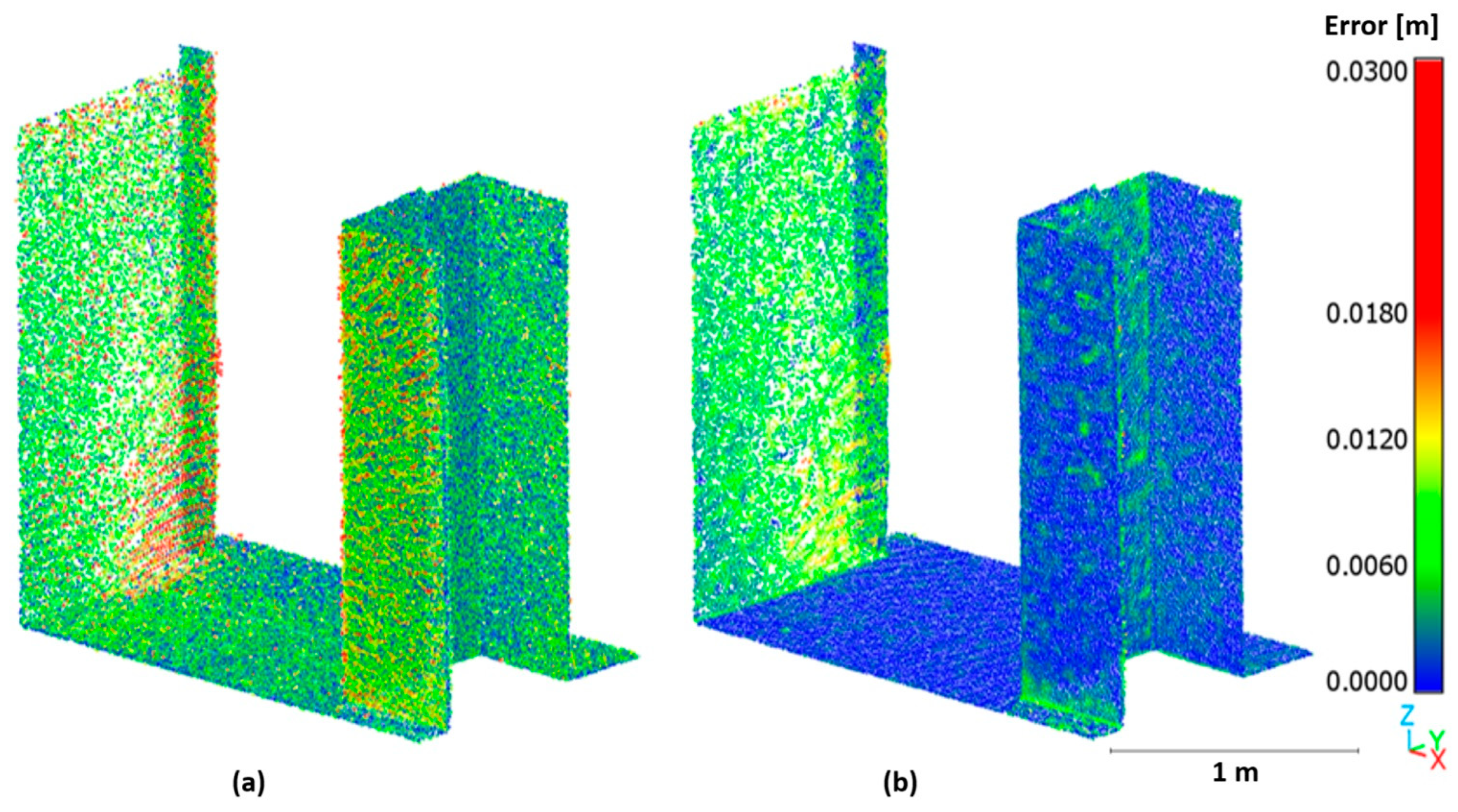
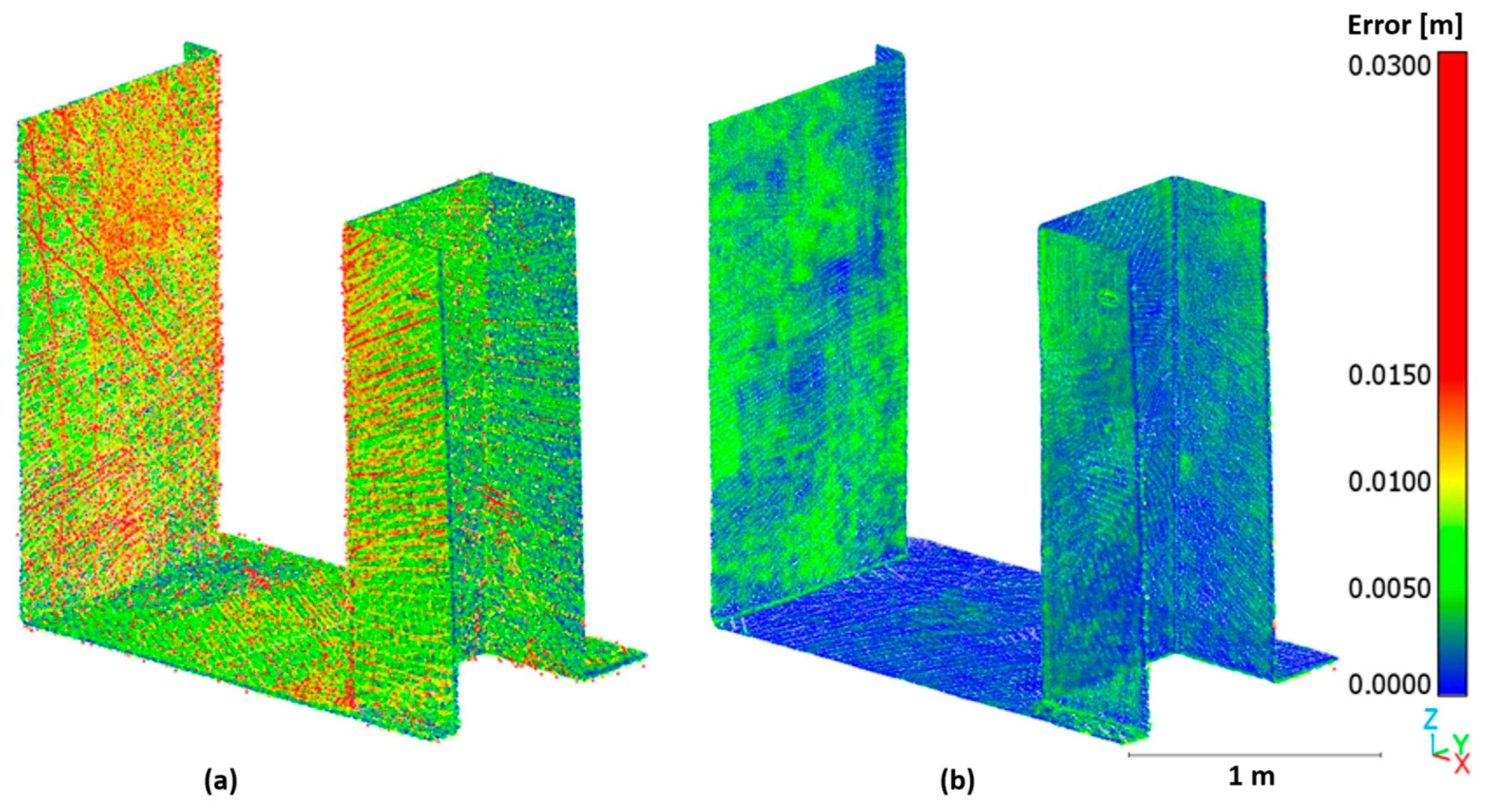
3.5. Visual Comparison of the Clouds

To illustrate the behavior of both the systematic and random error components, visual comparisons were prepared. The visualizations of SLAM scanner clouds were always based on the second passage. The figures always show the point clouds (a) transformed to spherical targets (their positions are shown in the figures) and (b) transformed using ICP. The respective RMSE values [m] are always shown in the upper part of the panel. Note that due to the differences in the maximum error values, the color coding of the errors (shown in the vertical bar next to each figure) could not be kept at an identical scale throughout all images.

The visualization of the Trimble X7 scanner clouds (Figure 9) shows a predominance of systematic (bending) error in this scanner. In the Figure 9a, showing the cloud transformed to spherical targets, the errors at the extreme ends are low due to the “pinning” of the cloud to the spherical targets, while the highest error can be observed in the middle. The Figure 9b presenting the result of ICP transformation shows an increase in the errors at the ends and a drop in the central part compared to the cloud (a). The maximum observed error was 2 cm.

In the point cloud acquired using Leica RTC 360 (Figure 10), the color-coding appears to indicate, at first sight, the presence of the systematic (shape) error. However, the fact that RMSE dropped only slightly after ICP transformation indicates the predominance of the random error. The maximum error is only 7 mm in this point cloud, which is the best value of all tested scanners.

In the point cloud acquired using the Emesent Hovermap ST-X (Figure 11), the random error predominates (likely due to the higher noise level). The maximum error is 3 cm.

The RMSE of the point cloud acquired by GeoSLAM ZEB Horizon RT (Figure 12) dropped by approx. 1/3 after the ICP transformation, which indicates that although a component of systematic error is present in the cloud, the random error predominates. The maximum error was the highest of all tested scanners (12 cm).

From the perspective of the error components, the FARO Orbis scanner (Figure 13) yielded a cloud with characteristics similar to the GeoSLAM ZEB Horizon RT. Random error predominated in that cloud as well, with RMSE dropping by about 25%. The maximum error of 4 cm was, however, notably smaller than in the case of GeoSLAM ZEB Horizon RT.

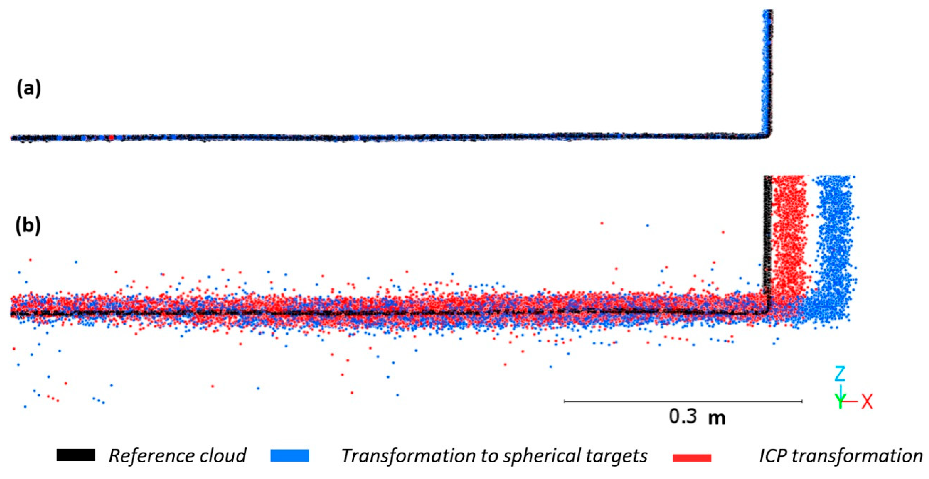
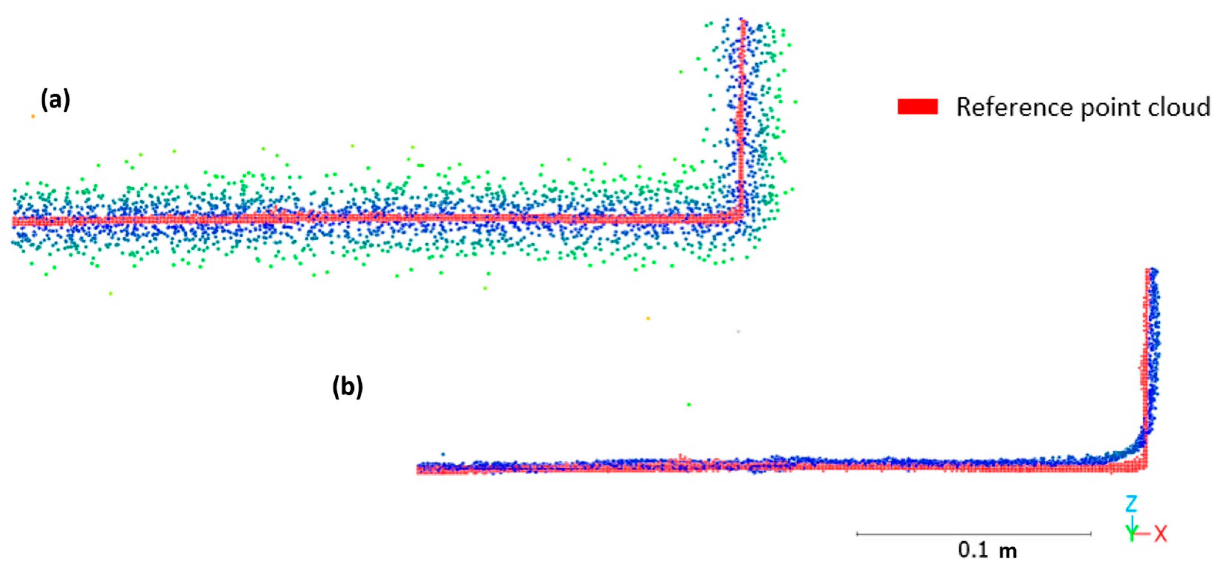
3.6. Local Accuracies in the Profiles

The local error and the displacement of each cloud relative to the reference cloud were evaluated in all three coordinate axes (X—transverse; Y—longitudinal; Z—height) on three profiles (see Figure 7). Only ICP-transformed clouds were evaluated.

Figure 14 presents the local behavior of the clouds after individual transformations on a detail of the central profile. In the Figure 14a, the difference between transformations is minimal, while in the Figure 14b, the difference is clearly visible, and the error remains high even after the ICP transformation.

3.7. Comparison of the Scanners

Table 4. Local accuracies (based on three profiles in the cloud) acquired as mean displacements from the ICP transformation matrix and standard deviation (StDev in the brackets).

Scanner	RMSE∅X (StDev) [mm]	RMSE∅Y (StDev) [mm]	RMSE∅Z (StDev) [mm]	RMSEMIN/MAX [mm] (Axis)	RMSEICP-PROFILE (StDev) [mm]
Trimble X7	8.8 (1.8)	0.6 (0.5)	1.2 (0.5)	10.0 (X)	1.2 (0.2)
Leica RTC 360	0.9 (0.5)	0.2 (0.3)	0.5 (0.6)	1.2 (X)	0.6 (0.1)
Emesent Hovermap ST-X	9.8 (5.6)	2.2 (2.2)	2.3 (2.3)	−18.2 (X)	5.5 (0.6)
GeoSLAM ZEB Horizon RT	71.1 (14.4)	10.7 (7.8)	4.2 (4.4)	−96.4 (X)	12.1 (0.7)
FARO Orbis	11.2 (5.7)	2.9 (2.7)	6.4 (2.9)	−18.0 (X)	5.2 (0.2)

RMSE_∅X—mean displacement in the X axis; RMSE_MIN/MAX (axis)—displacement with the maximum absolute value (and the affected axis); RMSE_∅Y—mean displacement in the Y axis; RMSE_∅Z—mean displacement in the Z axis; RMSE_ICP-PROFILE—mean error of the ICP-transformed profiles relative to the profiles from the reference cloud.

shows the mean displacements derived from the ICP transformation matrices for the three profiles and individual axes (∆X, ∆Y, ∆Z), along with the absolute value of the maximum observed displacement (∆_MAX), the axis of the maximum displacement, and the mean local accuracy of the cloud. The values always show means from all three profiles (and, in the case of SLAM scanners, also from all three measurements).

In all scanners, the highest displacement (error) was observed along the transverse (X) axis, followed by the vertical (Z) axis, and the least errors were observed in the longitudinal axis (Y). The GeoSLAM ZEB Horizon RT was the only exception, as the longitudinal error of its point cloud was greater than the height error. The best results were achieved by the Leica RTC 360 scanner, the maximum error of which in any of the coordinate axes never exceeded 1.2 mm (approx. 1% of the maximum error of the GeoSLAM ZEB Horizon RT approaching 10 cm).

With the exception of Emesent Hovermap ST-X, where the global and local error differed by only 0.3 mm (compare Table 4 and

Table 5. Mean RMSE values and standard deviation (StDev in the brackets) before smoothing, after smoothing, and noise for individual scanners.

Scanner	RMSEICP-local (StDev) [mm]	RMSEICP-local smoothed (StDev) [mm]	RMSEnoise (StDev) [mm]
Trimble X7	1.2 (0.2)	0.9 (0.1)	0.9 (0.2)
Leica RTC 360	0.6 (0.1)	0.7 (0.1)	-
Emesent Hovermap ST-X	5.5 (0.6)	2.2 (0.5)	5.0 (0.5)
GeoSLAM ZEB Horizon RT	12.1 (0.7)	7.6 (1.1)	9.3 (0.3)
FARO Orbis	5.2 (0.2)	2.1 (0.4)	4.7 (0.2)

), which indicates negligible systematic error and evenly distributed random error, the local accuracies of the other scanners (Table 4, RMSE_ICP-PROFILE) were better than global ones. The local accuracies also obviated the technological development of the scanners, especially in the SLAM scanners, where the newer generation (Emesent Hovermap ST-X and FARO Orbis) outperformed the older one (GeoSLAM ZEB Horizon RT).

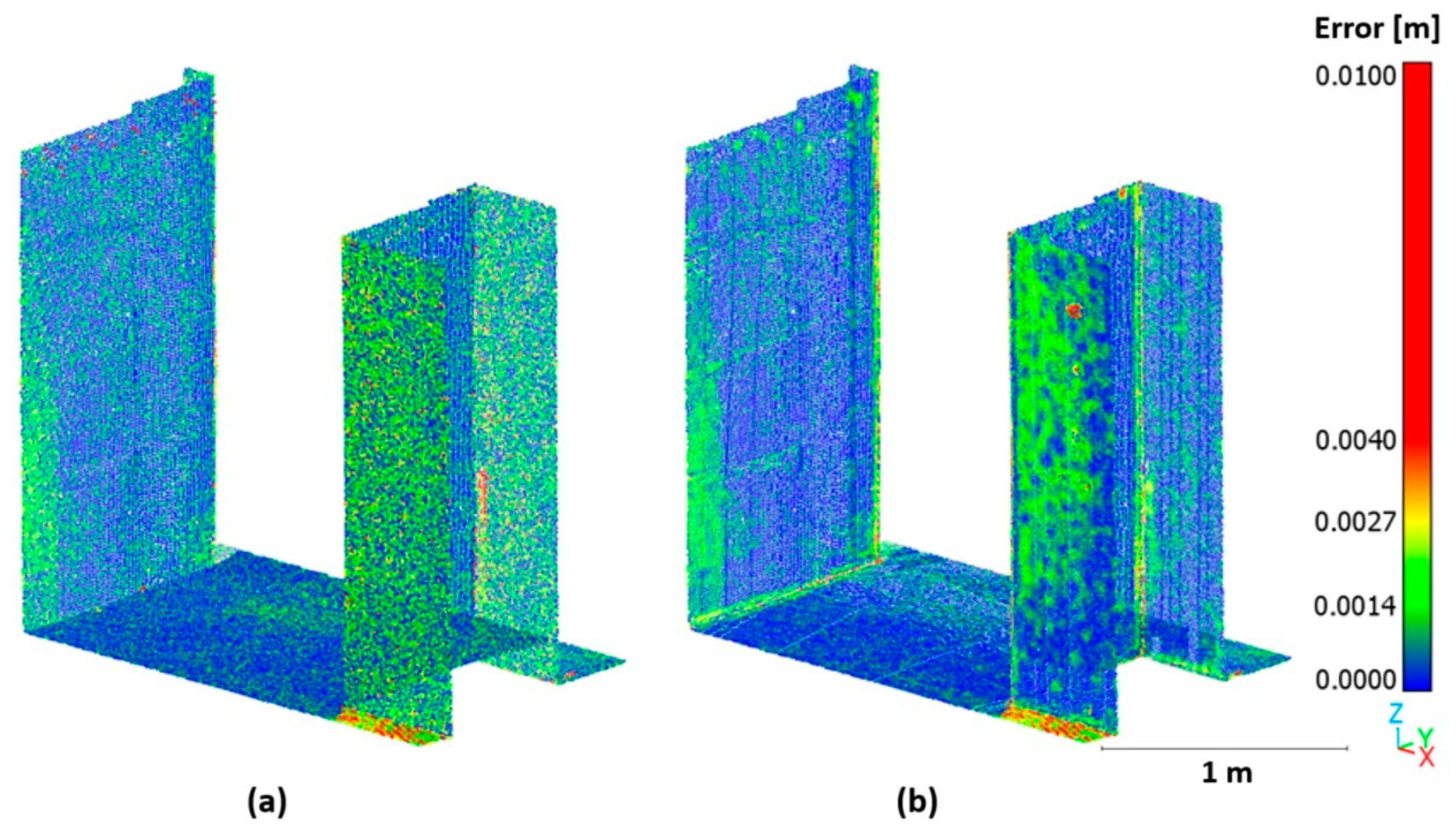
3.8. Comparison of Scanners from the Perspective of Noise

Table 5 shows the mean RMSE before smoothing, after smoothing, and noise levels for all scanners (means of all profiles and, in the case of SLAM scanners, also of all measurements).

The results clearly show that static scanners suffer from only a minimum noise. In the case of Leica RTC 360, smoothing even worsened the results, which prevented the noise calculation. On the other hand, GeoSLAM ZEB Horizon RT with its noise value of >9 mm performed the worst. SLAM scanners generally suffered from greater noise than static ones; after smoothing, however, the accuracies of the new-generation SLAM scanners were not far from that of static scanners. The technological advancement in the newer generations of SLAM scanners is obvious.

Figure 15 shows the effect of smoothing on GeoSLAM ZEB Horizon RT (Figure 15a—raw data, Figure 15b—after smoothing). The figure clearly demonstrates the benefit of smoothing on the noise reduction while, on the other hand, deteriorating the quality of sharp corners detection.

Visual Comparison

To better illustrate the numerical values, visual comparisons were added. The figures depict the clouds (a) before and (b) after smoothing. Note that color scales vary among scanners to reflect differing maximum RMSE values. The RMSE values shown in the figures are always valid for the particular depicted situation—the central profile in the static scanners and the central profile of the second measurement in SLAM scanners.

In static scanners, smoothing led to a minor improvement in accuracy, which was, however, at the cost of minor edge rounding and, therefore, a slight deterioration of the representativeness of the data. This is less pronounced in Trimble X7 (Figure 16) than in Leica RTC 360 (Figure 17).

In SLAM scanners, the improvement brought about by smoothing was greater than in static scanners, which was most noticeable in the vertical component. While Emesent Hovermap ST-X (Figure 18) and FARO Orbis (Figure 19) showed maximum errors of approx. 3 cm, the GeoSLAM ZEB Horizon RT, exhibited errors of up to 6 cm (Figure 20).

4. Discussion

Over the last years, SLAM scanners and their performance have become a focus of the expert community. SLAM technology was investigated, for example, in [28], where the quality of the resulting point clouds acquired using different SLAM algorithms was studied. The authors achieved accuracies of several centimeters to decimeters; however, the reported accuracies were only calculated based on manual measurement of several points in the study area, lacking the robustness required for a comprehensive statistical evaluation.

Fasiolo et al. [29] compared multiple algorithms for processing of SLAM data acquired using a SLAM scanner mounted on a robotic vehicle and compared the results with the reference cloud acquired using a terrestrial scanner. They achieved point cloud accuracies (RMSEs compared to the reference cloud) of approx. 0.05 m, increasing up to 0.1 m in a narrow walkway.

In [30], the GeoSLAM scanner was evaluated in underground environments, yielding RMSEs of 5–6 cm. The authors, however, did not compare the results to reference data—the comparison was limited to evaluation of the differences between two passes using the same scanner. In another study [31], Emesent Hovermap ST was tested in a similar environment, reporting accuracy of about 15 mm over approx. 45 m. It, however, needs to be mentioned that this value is not the absolute error but the error after ICP transformation (without any transformation to spherical points). When the same test was performed in a 150 m long corridor, however, Mean Absolute Deviation (MAD; relative to a reference cloud) increased to 0.1 m despite the ICP transformation (compare to 5.8 mm in our study at 80 m).

In another study [32], the Emesent Hovermap ST-X (the same version as in our paper; newer than in [31]) yielded a transverse accuracy of ~0.4 m at 750 m (one-way scan), improving to 0.1 m when a closed loop (i.e., round trip) was used for data acquisition.

In [33], three SLAM scanners were tested in underground spaces (approx. 75 m long) with walls made of shaped stones and bricks and compared with a terrestrial static scanner. GeoSLAM yielded an RMSE of 0.017 m; it, however, needs to be said that in that study, the transformation to reference data was always performed locally, no global result for the entire length of the space was reported.

A more comprehensive study [34] comparing the performance of multiple static and SLAM scanners in underground spaces to the reference data (Leica P40) reported RMSEs of SLAM scanners to be in the order of centimeters, which corresponds with the results of the current study. Another paper described the use of a SLAM scanner GeoSLAM REVO for scanning a castle and adjacent space [35], also reporting the errors of a few centimeters. Similar accuracies have been also reported in [36], where GeoSLAM ZEB Horizon RT was used for capturing a concrete bridge construction.

The accuracy of SLAM scanners in the interior of buildings was also discussed in [37], where it was combined with terrestrial scanning. Again, the accuracies were better than 0.05 m; it was, however, determined only using spatial distances between spherical targets placed in the individual rooms of the mapped indoor space.

Results of the tests performed in our study show that static scanners still remain the best choice for indoor measurements if accuracy is of paramount importance. The technological progress of SLAM scanners is, however, significant and with appropriate post-processing (e.g., ICP alignment and smoothing), these devices can deliver point cloud accuracies that are sufficient for most common surveying applications. Besides the speed of scanning, the fact that with SLAM scanners, occlusions are practically eliminated, represents an additional advantage of SLAM scanners.

These scanners present an interesting option for surveying indoor spaces due to their low weight, ease of manipulation, and, in particular, the short time needed for scanning. Of all tested SLAM scanners, Emesent Hovermap ST-X performed best, closely followed by FARO Orbis, which is characterized by a lower level of noise compared to Emesent Hovermap ST-X. This scanner, in addition, offers an important additional feature–surveying of reference points during scanning and their direct consideration in the measurement trajectory, which prevents the need for subsequent identification of reference points during post-processing and minimizes the introduction of further errors and improving accuracy. Of all tested scanners, the GeoSLAM ZEB Horizon RT performed worst; it is, however, necessary to point out that GeoSLAM ZEB Horizon RT is a representative of an older generation of scanners, both from the perspective of the software and scanning head.

Limitations of this study lie in the character of the testing area, which limits the generalizability of our results to the interior spaces with the character of corridors and should not be used to evaluate the performance of SLAM scanners in natural or outdoor environments. The total length of the corridor of 80 m can also be perceived as a limitation. On the other hand, this disposition is typical of residential as well as office buildings, for which the SLAM scanners are primarily intended.

5. Conclusions

This study compared the performance of static and SLAM scanners from various generations in a typical commercial indoor environment characterized by long, straight corridors with recesses. Although the static scanners achieved the highest accuracies (overall RMSE of 1.2 mm for Leica RTC360 and 5.4 mm for Trimble X7), new-generation SLAM scanners approached this accuracy (7.3 mm for Emesent Hovermap ST-X and 8.8 mm for FARO Orbis). This was a significant improvement when compared to the older generation scanner GEOSLAM ZEB Horizon RT with overall RMSE of 36.2 mm. These results were further confirmed in deeper analysis of local accuracies. Considering the fact that denoising of SLAM point clouds leads to further improvement of the accuracies and the rapid scanning when employing this type of instruments, we conclude that the use of new generation scanners already provides a highly suitable alternative to static scanners in indoor building environments.

References

1. Liu, J.; Azhar, S.; Willkens, D.; Li, B. Static Terrestrial Laser Scanning (TLS) for Heritage Building Information Modeling (HBIM): A Systematic Review. Virtual Worlds 2023, 2, 90–114. [Google Scholar] [CrossRef]
2. Wang, Y.; Chen, Q.; Zhu, Q.; Liu, L.; Li, C.; Zheng, D. A Survey of Mobile Laser Scanning Applications and Key Techniques over Urban Areas. Remote Sens. 2019, 11, 1540. [Google Scholar] [CrossRef]
3. Bolkas, D.; Guthrie, K.; Durrutya, L. sUAS LiDAR and Photogrammetry Evaluation in Various Surfaces for Surveying and Mapping. J. Surv. Eng. 2024, 150, 04023021. [Google Scholar] [CrossRef]
4. Vílchez-Lara, M.d.C.; Molinero-Sánchez, J.G.; Rodríguez-Moreno, C.; Gómez-Blanco, A.J.; Reinoso-Gordo, J.F. High Resolution 3D Model of Heritage Landscapes Using UAS LiDAR: The Tajos de Alhama de Granada, Spain. Land 2024, 13, 75. [Google Scholar] [CrossRef]
5. Polat, N. UAV-Based Investigation of Earthquake-Induced Deformation and Landscape Changes: A Case Study of the February 6, 2023 Earthquakes in Hatay, Türkiye. Earth Sci. Inform. 2023, 16, 3765–3777. [Google Scholar] [CrossRef]
6. Bartmiński, P.; Siłuch, M.; Kociuba, W. The Effectiveness of a UAV-Based LiDAR Survey to Develop Digital Terrain Models and Topographic Texture Analyses. Sensors 2023, 23, 6415. [Google Scholar] [CrossRef] [PubMed]
7. Kovanič, Ľ.; Peťovský, P.; Topitzer, B.; Blišťan, P. Complex Methodology for Spatial Documentation of Geomorphological Changes and Geohazards in the Alpine Environment. Land 2024, 13, 112. [Google Scholar] [CrossRef]
8. Komárek, J.; Lagner, O.; Klouček, T. UAV Leaf-on, Leaf-off and ALS-Aided Tree Height: A Case Study on the Trees in the Vicinity of Roads. Urban For. Urban Green. 2024, 93, 128229. [Google Scholar] [CrossRef]
9. Štroner, M.; Urban, R.; Křemen, T.; Braun, J. UAV DTM Acquisition in a Forested Area—Comparison of Low-Cost Photogrammetry (DJI Zenmuse P1) and LiDAR Solutions (DJI Zenmuse L1). Eur. J. Remote Sens. 2023, 56, 2179942. [Google Scholar] [CrossRef]
10. Fareed, N.; Flores, J.P.; Das, A.K. Analysis of UAS-LiDAR Ground Points Classification in Agricultural Fields Using Traditional Algorithms and PointCNN. Remote Sens. 2023, 15, 483. [Google Scholar] [CrossRef]
11. Moudrý, V.; Cord, A.F.; Gábor, L.; Laurin, G.V.; Barták, V.; Gdulová, K.; Malavasi, M.; Rocchini, D.; Stereńczak, K.; Prošek, J.; et al. Vegetation Structure Derived from Airborne Laser Scanning to Assess Species Distribution and Habitat Suitability: The Way Forward. Divers. Distrib. 2022, 29, 39–50. [Google Scholar] [CrossRef]
12. Pinpin, L.; Wenge, Q.; Yunjian, C.; Feng, L. Application of 3D Laser Scanning in Underground Station Cavity Clusters. Adv. Civ. Eng. 2021, 2021, 8896363. [Google Scholar] [CrossRef]
13. Rybansky, M. Determination of Forest Structure from Remote Sensing Data for Modeling the Navigation of Rescue Vehicles. Appl. Sci. 2022, 12, 3939. [Google Scholar] [CrossRef]
14. Strand, S.H.; Haakonsen, T.A.; Dahle, H.; Fan, H. Assessing the Measurement Quality of UAV-Borne Laser Scanning in Steep and Snow-Covered Areas. Int. Arch. Photogramm. Remote Sens. Spatial Inf. Sci. 2023, XLVIII-1/W2-2023, 757–764. [Google Scholar] [CrossRef]
15. Rocha, G.; Mateus, L.; Ferreira, V. Historical Heritage Maintenance via Scan-to-BIM Approaches: A Case Study of the Lisbon Agricultural Exhibition Pavilion. ISPRS Int. J. Geo-Inf. 2024, 13, 54. [Google Scholar] [CrossRef]
16. Choi, M.; Kim, M.; Kim, G.; Kim, S.; Park, S.-C.; Lee, S. 3D Scanning Technique for Obtaining Road Surface and Its Applications. Int. J. Precis. Eng. Manuf. 2017, 18, 367–373. [Google Scholar] [CrossRef]
17. Riveiro, B.; Morer, P.; Arias, P.; de Arteaga, I. Terrestrial Laser Scanning and Limit Analysis of Masonry Arch Bridges. Constr. Build. Mater. 2011, 25, 1726–1735. [Google Scholar] [CrossRef]
18. Lenda, G.; Marmol, U. Integration of High-Precision UAV Laser Scanning and Terrestrial Scanning Measurements for Determining the Shape of a Water Tower. Measurement 2023, 218, 113178. [Google Scholar] [CrossRef]
19. Lenda, G.; Kudrys, J.; Fryc, D. Sub-Centimetre Integration of Scanning Measurements: UAV and Terrestrial-Based, for Determining the Shape of a Shell Structure. Measurement 2023, 221, 113516. [Google Scholar] [CrossRef]
20. Keitaanniemi, A.; Rönnholm, P.; Kukko, A.; Vaaja, M.T. Drift Analysis and Sectional Post-Processing of Indoor Simultaneous Localization and Mapping (SLAM)-Based Laser Scanning Data. Autom. Constr. 2023, 147, 104700. [Google Scholar] [CrossRef]
21. Park, J.-I.; Park, J.; Kim, K.-S. Fast and Accurate Desnowing Algorithm for LiDAR Point Clouds. IEEE Access 2020, 8, 160202–160212. [Google Scholar] [CrossRef]
22. Chen, W.; Zhou, C.; Shang, G.; Wang, X.; Li, Z.; Xu, C.; Hu, K. SLAM Overview: From Single Sensor to Heterogeneous Fusion. Remote Sens. 2022, 14, 6033. [Google Scholar] [CrossRef]
23. Taheri, H.; Xia, Z.C. SLAM; Definition and Evolution. Eng. Appl. Artif. Intell. 2021, 97, 104032. [Google Scholar] [CrossRef]
24. Kumar Singh, S.; Pratap Banerjee, B.; Raval, S. A Review of Laser Scanning for Geological and Geotechnical Applications in Underground Mining. Int. J. Min. Sci. Technol. 2023, 33, 133–154. [Google Scholar] [CrossRef]
25. Gharineiat, Z.; Tarsha Kurdi, F.; Henny, K.; Gray, H.; Jamieson, A.; Reeves, N. Assessment of NavVis VLX and BLK2GO SLAM Scanner Accuracy for Outdoor and Indoor Surveying Tasks. Remote Sens. 2024, 16, 3256. [Google Scholar] [CrossRef]
26. Keitaanniemi, A.; Kukko, A.; Virtanen, J.-P.; Vaaja, M.T. Measurement Strategies for Street-Level SLAM Laser Scanning of Urban Environments. Photogramm. J. Finl. 2020, 27, 1–19. [Google Scholar] [CrossRef]
27. IEC 60825-1; Safety of Laser Products—Part 1: Equipment Classification and Requirements. International Electrotechnical Commision: Geneva, Switzerland, 2017.
28. Akpınar, B. Performance of Different SLAM Algorithms for Indoor and Outdoor Mapping Applications. Appl. Syst. Innov. 2021, 4, 101. [Google Scholar] [CrossRef]
29. Tiozzo Fasiolo, D.; Scalera, L.; Maset, E. Comparing LiDAR and IMU-Based SLAM Approaches for 3D Robotic Mapping. Robotica 2023, 41, 2588–2604. [Google Scholar] [CrossRef]
30. Wajs, J.; Kasza, D.; Zagożdżon, P.P.; Zagożdżon, K.D. 3D Modeling of Underground Objects with the Use of SLAM Technology on the Example of Historical Mine in Ciechanowice (Ołowiane Range, The Sudetes). E3S Web Conf. 2018, 29, 00024. [Google Scholar] [CrossRef]
31. Fahle, L.; Holley, E.A.; Walton, G.; Petruska, A.J.; Brune, J.F. Analysis of SLAM-Based Lidar Data Quality Metrics for Geotechnical Underground Monitoring. Min. Metall. Explor. 2022, 39, 1939–1960. [Google Scholar] [CrossRef]
32. Křemen, T.; Michal, O.; Jiřikovský, T.; Kuric, I. Long-distance SLAM scanning of mine tunnel—Testing of precision and accuracy of Emesent Hovermap ST-X. Acta Monstanistica Slovaca 2024, 29, 630–642. [Google Scholar] [CrossRef]
33. Di Stefano, F.; Torresani, A.; Farella, E.M.; Pierdicca, R.; Menna, F.; Remondino, F. 3D Surveying of Underground Built Heritage: Opportunities and Challenges of Mobile Technologies. Sustainability 2021, 13, 13289. [Google Scholar] [CrossRef]
34. Štroner, M.; Urban, R.; Křemen, T.; Braun, J.; Michal, O.; Jiřikovský, T. Scanning the underground: Comparison of the accuracies of SLAM and static laser scanners in a mine tunnel. Measurement 2025, 242, 115875. [Google Scholar] [CrossRef]
35. Sammartano, G.; Spanò, A. Point Clouds by SLAM-Based Mobile Mapping Systems: Accuracy and Geometric Content Validation in Multisensor Survey and Stand-Alone Acquisition. Appl. Geomat. 2018, 10, 317–339. [Google Scholar] [CrossRef]
36. Urban, R.; Štroner, M.; Braun, J.; Suk, T.; Kovanič, Ľ.; Blistan, P. Determination of Accuracy and Usability of a SLAM Scanner GeoSLAM ZEB Horizon: A Bridge Structure Case Study. Appl. Sci. 2024, 14, 5258. [Google Scholar] [CrossRef]
37. Keitaanniemi, A.; Virtanen, J.-P.; Rönnholm, P.; Kukko, A.; Rantanen, T.; Vaaja, M.T. The Combined Use of SLAM Laser Scanning and TLS for the 3D Indoor Mapping. Buildings 2021, 11, 386. [Google Scholar] [CrossRef]
Figure 1. (a) The schematic drawing of the technical floor (blue color indicates the extent of the reference point cloud obtained with Leica P40) and the used geodetic network (points 9001–9009). (b,c) Photos of the central part of the technical floor. (d) Example of a stabilized control point. The red and green arrows show the direction of the coordinate axes.
Applsci 15 08053 g001
Figure 2. (a) Layout of the technical floor with black and white targets (black 6001–6018) serving for the georeferencing of the Leica ScanStation P40 reference cloud and spherical targets (red 5001–5006) serving as reference points for all evaluated scanners. (b) Paper black and white target on the wall for Leica P40. (c) Black and white targets for Leica ScanStation P40 on a magnetic element. (d) The spherical target with a magnetic element. (e) The mounting platform for spherical targets. The area used for the test is shown in blue hatching.
Applsci 15 08053 g002
Figure 3. Instruments used for georeferencing and testing: (a) total station Trimble S9 HP; (b) static laser scanner Leica ScanStation P40; (c) static scanner Trimble X7; (d) static scanner Leica RTC360; (e) SLAM scanner Emesent Hovermap ST-X; (f) SLAM scanner GeoSLAM ZEB Horizon RT; and (g) SLAM scanner Faro Orbis.
Applsci 15 08053 g003
Figure 4. Approximate positions (black crosses) of the scanning stations of the static scanners.
Applsci 15 08053 g004
Figure 5. Schematic drawing of the SLAM scanner trajectories (black arrows indicate the movement direction).
Applsci 15 08053 g005
Figure 6. Illustration of the two types of error in the shape of the point cloud (the size of error is characterized by the vertical deviation from the reference cloud–black line). Random error (blue line) remains similar along the entire cloud (i.e., along the scanned path), while the systematic error is lowest at the terminal points (where it is “pinned” to GCPs) and highest in the middle of the path. ICP transformation aims to minimize the overall error, which leads to approx. halving both the maximum and overall errors.
Applsci 15 08053 g006
Figure 7. Position of the profiles (1, 2, 3) for accuracy assessment (highlighted in blue).
Applsci 15 08053 g007
Figure 8. Examples of spherical targets scanned by individual scanners. (a) Trimble X7; (b) Leica RTC 360; (c) Emesent Hovermap ST-X; (d) GeoSLAM ZEB Horizon RT; (e) FARO Orbis (f) Leica ScanStation P40.
Applsci 15 08053 g008
Figure 9. The visualization of the errors of the cloud acquired using Trimble X7 (a) after transformation to spherical targets (RMSEOVERALL = 5.4 mm); and (b) after ICP transformation (RMSEICP-ALL = 2.5 mm).
Applsci 15 08053 g009
Figure 10. The RMSEs of the Leica RTC 360 (a) after transformation to spherical targets (RMSEOVERALL = 1.2 mm); and (b) after ICP transformation (RMSEICP-ALL = 1.0 mm).
Applsci 15 08053 g010
Figure 11. The RMSEs of the Emesent Hovermap ST-X (a) after transformation to spherical targets (RMSEOVERALL = 7.3 mm); and (b) after ICP transformation (RMSEICP-ALL = 5.8 mm).
Applsci 15 08053 g011
Figure 12. The RMSEs of the GeoSLAM ZEB Horizon RT (a) after transformation to spherical targets (RMSEOVERALL = 35.3 mm); and (b) after ICP transformation (RMSEICP-ALL = 21.9 mm).
Applsci 15 08053 g012
Figure 13. The RMSEs of the FARO Orbis (a) after transformation to spherical targets (RMSEOVERALL = 8.2 mm); and (b) after ICP transformation (RMSEICP-ALL = 6.0 mm).
Applsci 15 08053 g013
Figure 14. Detail of the central profile after transformations to spherical targets and ICP transformation for (a) Leica RTC 360; and (b) GeoSLAM ZEB Horizon RT.
Applsci 15 08053 g014
Figure 15. The effect of smoothing on GeoSLAM ZEB Horizon RT: (a) before smoothing; (b) after smoothing. Red dots are reference point cloud, blue and green dots represent compared point cloud (shade given by distance).
Applsci 15 08053 g015
Figure 16. Profile 2 acquired by Trimble X7 (a) before (RMSEICP-Local = 1.1 mm); and (b) after smoothing (RMSEICP-Local smoothed = 0.9 mm).
Applsci 15 08053 g016
Figure 17. Profile 2 acquired by Leica RTC 360 (a) before (RMSEICP-Local = 0.7 mm); and (b) after smoothing (RMSEICP-Local smoothed = 0.8 mm).
Applsci 15 08053 g017
Figure 18. Profile 2 acquired by Emesent Hovermap ST-X (a) before (RMSEICP-Local = 5.9 mm); and (b) after smoothing (RMSEICP-Local smoothed = 2.6 mm).
Applsci 15 08053 g018
Figure 19. Profile 2 acquired by FARO Orbis (a) before (RMSEICP-Local = 5.4 mm); and (b) after smoothing (RMSEICP-Local smoothed = 2.2 mm).
Applsci 15 08053 g019
Figure 20. Profile 2 acquired by GeoSLAM ZEB Horizon RT (a) before (RMSEICP-Local = 11.9 mm); and (b) after smoothing (RMSEICP-Local smoothed = 7.4 mm).
Applsci 15 08053 g020