Integration of Space and Hydrological Data into System of Monitoring Natural Emergencies (Flood Hazards)

Abstract

Flood hazards have increasingly threatened the East Kazakhstan region in recent decades due to climate change and growing anthropogenic pressures, leading to more frequent and severe flooding events. This article considers an approach to modeling and forecasting river runoff using the example of the small Kurchum River in the East Kazakhstan region. The main objective of this study was to evaluate the numerical performance of the flood hazard model by comparing simulated flood extents with observed flood data. Two types of data were used as initial data: topographic data (digital elevation models and topographic maps) and hydrological data, including streamflow time series from stream gauges (hourly time steps) and lateral inflows along the river course. Spatially distributed rainfall forcing was not applied. To build the model, we used the software packages of HEC-RAS version 5.0.5 and MIKE version 11. Using retrospective data for 3 years (2019–2021), modeling was performed, the calculated boundaries of possible flooding were obtained, and the highest risk zones were identified. A dynamic map of depth changes in the river system is presented, showing the process of flood wave propagation, the dynamics of depth changes, and the expansion of the flood zone. Temporal flood inundation mapping and performance metrics were evaluated for each individual flood event (2019, 2020, and 2021). The simulation outcomes closely correlate with actual flood events. The assessment showed that the model data coincide with the real ones by 91.89% (2019), 89.09% (2020), and 95.91% (2021). The obtained results allow for a clarification of potential flood zones and can be used in planning measures to reduce flood risks. This study demonstrates the importance of an integrated approach to modeling, combining various software packages and data sources.

1. Introduction

In recent decades, climate change has led to an increase in the number of natural disasters both around the world and in East Kazakhstan [1,2,3]. These processes increase the risk of avalanches in winter and floods in spring, which requires new solutions for their monitoring. Thus, an automated avalanche hazard monitoring system is being created for Eastern Kazakhstan. The initial data for modeling and their results for flood forecasting can be included in the existing database as a development and continuation of the project [4]. Monitoring the flood situation along with avalanche monitoring can complement the regional system for monitoring natural disasters.

According to statistics from the Department of Emergency Situations of the East Kazakhstan region for 2023 [5], the level of potential flood threats has decreased in a number of areas. In total, there are about 71 settlements in East Kazakhstan that are prone to flooding. In 15 settlements, the threat has been completely removed and minimized in 46. Despite this, floods, as a natural disaster, remain a pressing problem. During the flood period, increased attention is paid to the following areas of the East Kazakhstan region due to the high amount of danger: Altai, Glubokoe, Ulan, Shemonaikha, Tarbagatai, Katon-Karagay, and Zaysan. Taking into account the freezing of the soil and the height of the snow cover, with a sharp increase in temperature and heavy precipitation, the flood situation may worsen.

The flood hazard monitoring system helps to minimize losses from seasonal floods [5], and it is also planned to integrate the flood hazard system and the snow monitoring system.

At the same time, the problems of managing and monitoring river systems have become especially relevant due to the increasing anthropogenic load and increasing demand for water resources. Effective management of river flows requires complex information and analytical systems capable of promptly processing and providing data for decision-making. The basis of such systems is modeling tools that allow for highly accurate predictions of the behavior of river flows under various conditions.

Due to the widespread occurrence of the danger of floods in almost every country with the necessary scientific and technical potential, the territory of which is exposed to this danger, there are teams or even entire institutes working purposefully to study and forecast river flows and design and build protective engineering structures.

Currently, methods of numerical modeling of river flows based on various mathematical models are widely used. Many researchers determine the flood zone based on hydrodynamic modeling using modern HEC-RAS 5.0 software. In [6], a model based on satellite data on precipitation was used, while hydrodynamic modeling in RAS 5.0.5 and HEC-HMS 5.0 software is used, which allows for simulating flow regimes and hydrological characteristics. The modeling results made it possible to predict the increase in the water level in two river tributaries within the Citarum River watershed. In the work by the authors Sumiadi, B. Winarta, D. et al. [7], for flood modeling, HEC-RAS 5.0 with Q25y and Q50y is also used, and a model is built on the basis of data obtained as a result of an analysis of precipitation data from 9 observation stations.

In a study by the authors Zhu H. and Chen Y. [8], methods of hydrological modeling of watersheds are also applied for flood forecasting. In addition, a digital elevation model (DEM) is considered as an input variable, which, due to the resolution (in the range of 30 m to 500 m), significantly affects the accuracy of flood modeling. The modeling is based on a hydrological and hydraulic analysis using the HEC-RAS 4.1.0 program. Researchers from Indonesia [9] studied precipitation (rain) data obtained from Pengelolaan Sumber Daya Air (PSDA) and the spatial data of Brebes County from 2009 to 2018, and by normalizing these data (using lognormal distribution), the probability of flooding of the county was calculated.

The authors of the article [10] presented a 2D modeling concept created in their study, whereby a cascade of 25 2D models was developed in the MIKE21 software, which covers a 600 km-long stretch of the Odra River (Poland) with an area of 5700 km². A constant grid resolution of 4–6 m was used in the modeling. The models were applied for multiple purposes, first to develop the flood hazard and risk maps for major cities, then to validate historical flood data and stage–discharge relationships at monitoring stations and to verify design discharges through flood routing.

In a study by Lyu X., Li Z., Li X. [11], the applicability of hourly data from the Global Precipitation Measurement Mission (GPM) Integrated Multi-satellite Retrievals for GPM (IMERG V6 and IMERG V7) for event-based flood modeling in the Songshui River basin in southwest China using the hydrological modeling system (HEC-HMS) was assessed. Land stations were used to adjust the data, which significantly improved the accuracy of flood modeling.

The paper [12] presents two empirical methods for predicting downstream hydraulic variables based on observed flow data: a linear programming (LP) model and a convolutional neural network (CNN). In this paper, we apply both empirical models to the Colorado River system at a site on the Green River downstream of the Yampa River confluence and Flaming Gorge Dam and compare it with the physics-based Streamflow Synthesis and Reservoir Regulation (SSARR) model. The results show that both proposed models significantly outperform the SSARR model. Moreover, the CNN model outperforms the LP model for hourly forecasts, while both perform similarly for daily forecasts.

In [13], the applicability of the k-nearest neighbor (KNN) algorithm for forecasting the mean daily discharge of the Ramis River at the Ramis gauging station is investigated. A dataset including the basin-wide mean rainfall and the mean daily discharge obtained from hydrometeorological stations with different lags was used as input to the KNN machine learning algorithm. The performance of the KNN algorithm was quantitatively evaluated using hydrological capability metrics, such as the mean absolute percentage error (MAPE), anomaly correlation coefficient (ACC), Nash–Sutcliffe efficiency (NSE), Kling–Gupta efficiency (KGE’), and spectral angle (SA). The flow forecasting results of the Ramis River using the k-nearest neighbor machine learning algorithm achieved a high level of reliability with flow lags of one and two days and precipitation of three days.

The authors of the study [14] showed that 1D flood modeling overestimated water depth and flow velocity compared to 2D flood modeling. This is due to the fact that the 2D model used an implicit algorithm for determining the final volume, which is more accurate and stable compared to 1D modeling.

The authors of the work [15] emphasize that the highest peak flow results were obtained using the HEC-HMS method among the three SUH formulas and HEC-RAS calculations. The deviation of the peak flow value using SUH, HEC-HMS, and HEC-RAS was less than 10%.

At the same time, the authors of the work [16] used an integrated modeling approach to combine the soil and water assessment tool (SWAT 2012 version) and the river analysis system of the Hydrological Engineering Center (HEC-RAS 5.0.7 version). SWAT was used to generate the effective rainfall amounts required to run 2D rainfall hydrodynamic simulations on the HEC-RAS grid.

The approach presented by the authors in [17] is also noteworthy, who studied hydrological analyses using the HEC-HMS software and flood analyses using HEC-RAS (Ras Mapper). As a result of the HEC-HMS modeling, a flood flow restoration plan was obtained for 5, 10, and 25 years, which was 185 m³/s, 208.7 m³/s, and 234.3 m³/s. The results of the HEC-RAS modeling show that the flooded area with repeated flood flows after 5, 10, and 25 years was 857.08 ha, 885.62 ha, and 979.59 ha.

The authors of [18] digitized the maps of their study area using the AutoCAD Civil 3D 2020 program, and cross-sections were made by obtaining digital elevation models of the region. The obtained cross-sections were defined in the HEC-RAS software, and the floodplain channel’s hydraulic characteristics and water surface profiles for the Q25, Q50, Q100, and Q500 recurring floods were determined, and a one-dimensional analysis of the Tigris River floodplain was carried out.

Thus, many studies show a variety of approaches to solving problems, but no single solution has been developed. Most researchers only consider meteorological data and river topology, but when modeling a particular region of the world, it is necessary to consider broader datasets.

This study is among the first to integrate spatial remote sensing data (Sentinel-1 and Sentinel-2) with hydrodynamic modeling based on the Saint–Venant equations for East Kazakhstan. This integration significantly improves the accuracy and timeliness of flood risk predictions and enhances the capabilities of the regional flood hazard monitoring system. In this study, we applied a subset of these data, including satellite imagery (Sentinel-1 and Sentinel-2), digital elevation models, topographic maps, and streamflow data from gauging stations. Snow storage and meteorological data were collected and maintained in the avalanche hazard monitoring subsystem, which is part of the integrated regional monitoring system.

The objective of this study was to evaluate the numerical performance of the flood hazard model by comparing simulated flood extents with observed flood data based on space monitoring data and hydrodynamic modeling of river flows using the MIKE software package, with subsequent scaling of the obtained results to assess flood risks in a larger river network of the East Kazakhstan region.

This study simulated flooding on one typical small river and extrapolated the obtained modeling results to a larger river network. This approach is feasible and important, because small rivers can serve as representative models for hydrodynamic processes in the region. Their simpler geometry and relatively better availability of data allow for robust calibration and validation of the model, which can then be efficiently scaled to larger and more complex river systems, particularly in regions where hydrological and topographical data for large networks are limited.

The relevance of this work lies in the study conducted to forecast and model the river runoff of the small Kurchum River in the East Kazakhstan region and the extension of the obtained data to the river network, and it is shown how the integration of various data allows for more accurate modeling of flood developments and clarifications of flooded areas.

Modeling flood risks for small rivers is a complex task, since the amount of input data is limited. The researchers of [19] were engaged in solving similar problems using the example of a small river (the Tarna River) from 1990 to 2019. Their assessment focused on modeling, as well as model calibration and validation using event-based time series data under poor data conditions. The authors of [19] did not consider the problem of extending their model to a river network.

Two types of data were considered and applied to model the river flow: topographic data (digital elevation models (DEMs), topographic maps, a hydrographic network, floodplain zones, and adjacent areas) and hydrological data, including streamflow time series from stream gauges with an hourly time step, flood hydrographs, and lateral inflow data. Spatially distributed rainfall forcing was not applied.

At the same time, flood mapping is required to determine flood characteristics such as flow velocity, flood depth, and degree of flooding; this is a prerequisite for flood management planning. Using HEC-RAS version 5.0.5 and an example of flood calculations for one river allowed for analyzing flooding as a result of a model flood.

2. Materials and Methods

Depending on the causes of occurrence, five groups of floods are distinguished, each of which is associated with certain natural or man-made factors.

Table 1. Flood classification.

Group	Description of the Group
1st group	This group includes floods associated mainly with the maximum runoff from spring snowmelt. Such floods are characterized by a significant, fairly long-term rise in the water level in the river and are usually called high-water floods.
2nd group	This group includes floods formed by intense rains, sometimes by melting snow during winter thaws. They are characterized by intense, relatively short-term rises in the water level and are called freshets.
3rd group	This group includes floods caused mainly by the high resistance that the water flow encounters in the river. This usually occurs at the beginning and end of winter during ice jams.
4th group	This group includes floods created by wind surges of water on large lakes and reservoirs, as well as in sea estuaries.
5th group	This group includes floods due to dam breaks.

shows the classification of floods.

Over the past 30 years, the East Kazakhstan region has seen a predominance of floods of groups 1 and 2. This conclusion was derived during an analysis of historical flood data for the East Kazakhstan region, based on official records and data provided by the Republican State Enterprise “Kazhydromet” [20] and the Department for Emergency Situations of the East Kazakhstan region [21]. To forecast and monitor the flood situation, the emergency monitoring system was used, which is a comprehensive tool that includes many modules for processing, modeling, and visualizing data (Figure 1).

These modules work closely together to effectively analyze and respond to potential threats [22]. The system includes a graphical database that is filled by receiving information on the current state of flood zones and the dynamics of their development using space monitoring systems. This monitoring technology is based on an analysis of EOS-AM TERRA MODIS daytime images and Sentinel-2 [23] space images and allows for tracking the dynamics of flood zones during floods and inundations. At the second level, medium-resolution data, such as Landsat, as well as radar data are used as they are received. At the third level, when it is necessary to analyze the situation in particularly critical cases, high- and ultra-high-resolution optical and radar remote sensing data (RSD) are used [24]. By superimposing flood zones on these layers, the system can quickly identify objects under threat. Among the key elements of the system, it is worth highlighting the data analysis module. This component is especially designed for modeling river flows and contains a number of modules, each of which performs its own function of modeling and forecasting floods.

Currently, there are many software solutions for modeling hydrodynamic processes on the market. However, when it comes to forecasting and preventing natural disasters, special attention is paid to software packages such as HEC-RAS and MIKE [25]. To create a simulation model of a river (canal) system, it is necessary to know hydraulics, numerical methods used in computational hydraulics, differential and integral calculus, programming, and data processing principles. In this study, a numerical modeling method based on the description of motion by the Saint–Venant equations was chosen [26]. When solving problems using the Saint–Venant equations, problems arise with the insufficiency and low accuracy of the initial information, primarily hydraulic resistance. The flow in the channel is considered one-dimensional (although purely one-dimensional flows do not exist in nature). In reality, a distinction is made between flows in the channel and on the floodplain. On the floodplain, the flow is more complex than in the channel and is more difficult to describe. Most often, the role of floodplains in the propagation of a flood wave consists of the accumulation of additional volume with weak water exchange between its individual parts. Usually, rivers are modeled on a scale that allows for an enlarged, rough schematization of floodplains. If it is necessary to represent floodplain details with greater accuracy, physical modeling is used or two-dimensional modeling is used.

The hydrodynamic modeling presented in this study is based on the one-dimensional Saint–Venant equations. These equations are fundamental in hydraulic engineering for simulating unsteady open-channel flows and describe the conservation of mass (continuity equation) and momentum for gradually varied flow conditions.

The continuity equation ensures that the total volume of water is conserved along the river, while the momentum equation accounts for the balance of forces acting on the flow, such as gravity, pressure, and channel resistance. These physical principles allow the equations to capture how water moves and changes depth over time and distance.

The Saint–Venant equations provide a reliable mathematical basis for predicting water levels, flow velocities, and flood inundation extents in riverine environments [27,28]. In this study, the Saint–Venant equations were applied using the MIKE 11 software environment, which implements numerical solutions based on finite difference schemes. By applying the Saint–Venant equations, the aim was to provide accurate flood hazard assessments that can inform flood risk management and emergency response planning for the East Kazakhstan region.

To justify the choice of simulation tools, a comparison of commonly used hydrodynamic modeling software packages was conducted (

Table 2. Comparison of selected 1D/2D flood modeling software packages.

Feature	MIKE (DHI)	HEC-RAS	LISFLOOD-FP	TUFLOW
Hydrodynamic model	Full 1D/2D Saint–Venant, flexible coupling	1D/2D Saint–Venant	Simplified hydrodynamics	Full 1D/2D Saint–Venant
GIS integration	High (direct integration and flexible data input)	Medium (requires preprocessing)	Limited	High
Data input options (e.g., satellite and DEM)	Direct support, high-resolution DEMs, and remote sensing	DEM-based and limited remote sensing support	DEM-based	DEM-based
Handling of complex river–floodplain systems	Strong (tested in complex systems worldwide)	Moderate (requires careful setup)	Limited for complex geometry	Strong
Interface usability	User-friendly and advanced visualization	Moderate	Simple command line	Moderate
Computational efficiency	High (optimized solvers and parallel computing)	Moderate	Very high for simple cases	High
License	Commercial	Free	Free	Commercial

). At the initial stage of this study, both HEC-RAS 5.0.5 and MIKE 11 were considered. HEC-RAS was used for exploratory simulations to evaluate basic hydraulic behavior and boundary conditions. However, all final hydrodynamic simulations, flood mapping, and result analyses presented in this study were performed using the MIKE 11 software. The decision to proceed with MIKE 11 was made due to its superior flexibility, numerical stability, and integration capabilities with remote sensing and GIS data, which were essential for the complex floodplain conditions of the Kurchum River basin. MIKE was selected as the most suitable tool for this study due to its advanced capabilities for simulating complex river–floodplain systems, strong integration with GIS and remote sensing data, a user-friendly interface, and proven accuracy in similar applications. This choice ensures high precision and flexibility in modeling flood dynamics under the specific conditions of the East Kazakhstan region.

The study examines an analytical module designed to calculate the degree of flooding of territories in the event of hydrodynamic disasters that occur as a result of emergency breakthroughs. Such events are characterized by rapid flooding of the area as a result of the formation of a breakthrough wave. The size and consequences of these accidents largely depend on many factors, including the parameters and condition of hydraulic structures; the nature and scale of dam failures; the volume of water in reservoirs; the characteristics of the breakthrough wave and flood; terrains; as well as time factors, such as the season and time of day [29].

The main destructive agents in catastrophic flooding are the breakthrough wave, determined by the height and speed of movement, as well as the duration of the flood. A breakthrough wave is a powerful flow of water formed by a sudden discharge of water from an upper level to a lower one, which causes its overflow and the formation of a high and fast-moving wave with destructive force. This wave differs from ordinary wind waves, as it is capable of carrying significant volumes of water in the direction of its movement, constantly changing its shape, size, and speed. The destructive effect of a breakthrough wave is due to a number of factors, including a sharp change in the water level during the destruction of hydraulic structures, the impact of a moving mass of water, changes in soil characteristics under the influence of water, erosion and soil movement, as well as the movement of debris from buildings and structures at high speeds. The breakthrough wave generates significant hydrodynamic loads on structures and the surrounding environment, which can lead to severe damage. At the initial stage, the front of a breakthrough wave, moving at a high speed, can have a steep shape, especially near the destroyed hydraulic structure, and can become gentler at a greater distance from the source of the breakthrough.

This article presents a hydraulic model in the MIKE program, demonstrating a simulated section of the Kurchum River in the East Kazakhstan region.

Accurate and reliable initial data, including topographic, hydrological, geometric, and boundary parameters, were prepared as described above.

Topographic data (digital elevation models and maps) were used to define terrain and hydrographic features. These data were converted into a computational grid, setting the basis for further hydrodynamic calculations. In this study, the DEM provided a detailed 3D terrain model, while topographic maps were used to verify and complement DEM data for hydrographic features. River bathymetry was derived from the DEM, as no separate bathymetric measurements were available.

Hydrological data consist of time series of water levels, discharges, and lateral inflows, as well as flood hydrographs. These data allow us to take into account the dynamics of water inflows into a river network and changes in water levels over time [30].

For example, a water flow hydrograph can be presented as a time series, where, for each time step, the volume of water passing through a given river section is specified. In addition to this, data on water inflows from lateral basins are used, which are specified as a linear inflow along the channel. Hydrological data are usually obtained from observations at hydrological posts or calculated using specialized precipitation–runoff models. These parameters are specified through the Boundary Editor and Time Series Editor modules, where dynamic conditions for the upper and lateral boundaries are formed.

To assess the quality of the hydrodynamic flood model, it is necessary to calculate the degree of coincidence of the simulated flood zones with the actually observed zones. For this purpose, the open source QGIS 3.16 software is used in this work [31]. The images were loaded into QGIS, georeferencing was performed, and the area of each flood polygon was calculated. QGIS allows you to calculate the areas of polygons using the built-in Field Calculator. The area of the polygon is calculated using Formula (1):

$$S={\sum }_{i=1}^n{A}_i$$

(1)

where S is the total area of the polygon (km² or m²), and A_i is the area of individual polygons included in the flood zone. Each polygon is on average 0.5 km². In total, there are 74 polygons in the actual flooded area. Based on these data, the total area of the actual flooded zone for spring 2019 is as follows:

$$S_{real}={\sum }_{i=1}^{74}0.5 \approx 37 {\mathrm{km}}^2$$

(2)

It is important to take into account that in real conditions the area of each polygon may vary, which is taken into account in automatic calculations of QGIS using the Field Calculator tool. This approach allows for a flexible analysis of flood distribution.

Using the same method, we calculated the area of the simulated flooded territory for 68 flood polygons for spring 2019:

$$S_{flood}={\sum }_{i=1}^{68}0.5 \approx 34 {\mathrm{km}}^2$$

(3)

To assess the accuracy of the model, the percentage of coincidence of the modeled territory with the real flood zone was calculated using the following formula:

$$Match percentage \left(\%\right)={\displaystyle \frac{S_{flood}}{S_{real}}}\times 100\%\approx 91.89\%$$

(4)

The obtained percentage of coincidence of 91.89% for spring 2019 indicates sufficient accuracy of the hydrodynamic model. The calculation error is 8.1%.

Following the methodology described earlier, the corresponding percentage of coincidence was calculated for the 2020 and 2021 flood events, where for 2020, the observed flood area was 26.6 km², and the modeled flood area was 23.7 km², with a degree of coincidence of 89.09%, and for 2021, the observed flood area was 18.8 km², and the modeled flood area was 19.6 km², with a degree of coincidence of 95.91%.

3. Results and Discussion

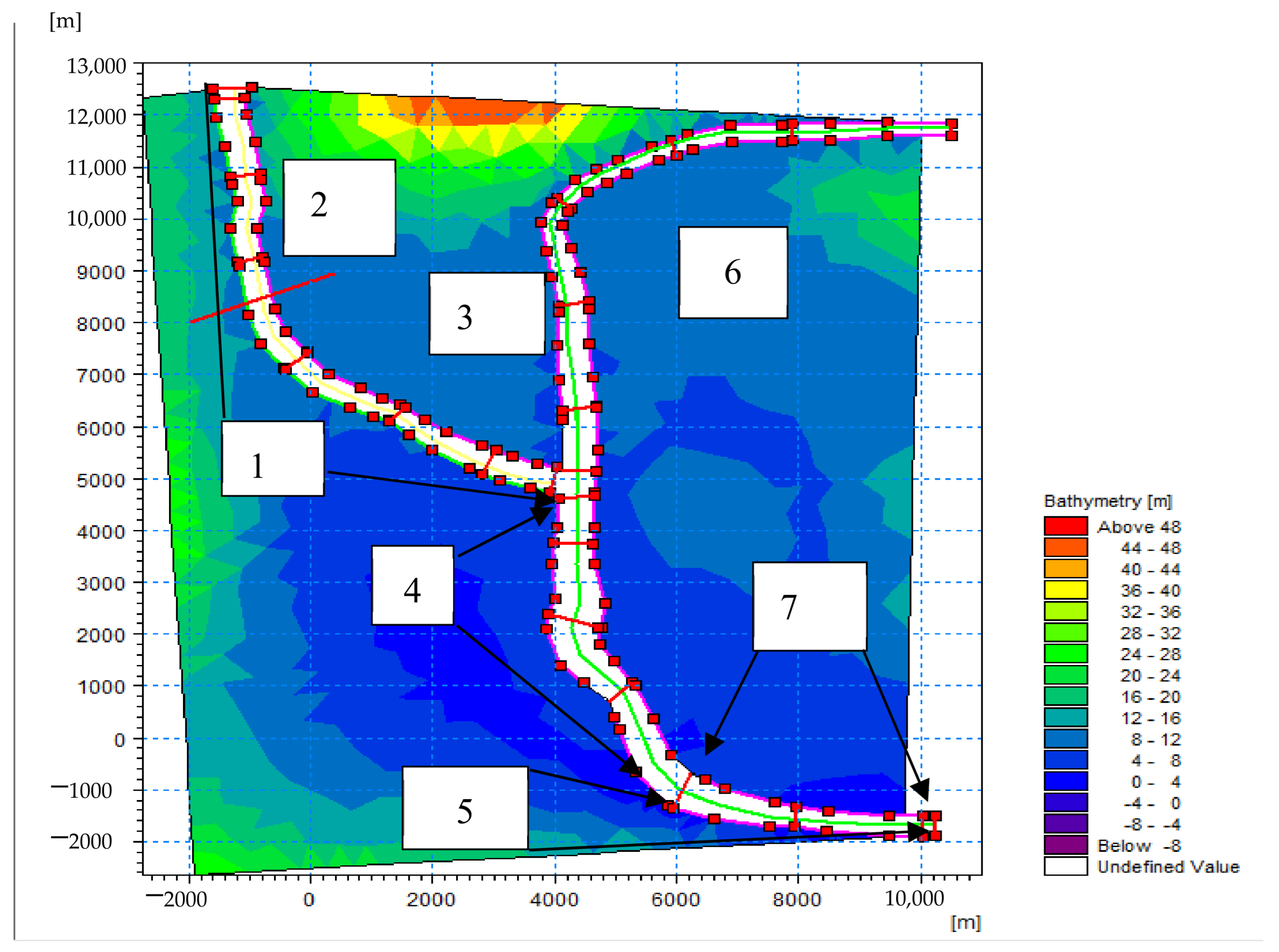
The geometry of the river network is the next important aspect of modeling. It describes the physical characteristics of the channel and its relationship with the adjacent territory. To build a model, it is necessary to determine the structure of the river network, including nodes, sections, and connections between them. Each section of the network is characterized by the length, flow direction, and connections with neighboring sections. The most important element of the geometry is cross-sections, which describe the shape of the channel at certain points. A cross-section includes the coordinates of the points that define the profile of the river bottom and banks, as well as the parameters of the channel roughness, such as the Manning’s n coefficient.

Table 3. Table of coordinates of linear sections of the river (coordinates).

N	Right Bank of the Tributary			Left Bank of the Tributary
	X	Y	Chainage	X	Y	Chainage
1	−1610.4390	12,500.1638	90,000.0000	−954.4890	12,537.2931	90,000.0000
2	−1581.8168	12,313.0126	90,200.0000	−1096.5935	12,340.4780	90,200.0000
3	−1539.9760	11,949.8690	90,563.3249	−1055.9717	12,012.5306	90,563.3249
4	−1396.6511	11,409.0343	91,148.1297	−910.6176	11,481.0048	91,148.1297
5	−1304.8629	10,815.7874	91,800.0000	−812.0049	10,861.7874	91,800.0000
6	−1292.3875	10,657.7992	91,947.4726	−810.7010	10,741.6631	91,947.4726
7	−1213.7016	10,339.4039	92,330.9679	−740.9593	10,359.1484	92,330.9679
8	−1315.6180	9815.3727	92,901.4439	−866.0027	9823.2054	92,901.4439
9	−1200.0251	9165.1282	93,550.0000	−785.7148	9250.4274	93,550.0000
10	−1183.7913	9091.2438	93,638.1801	−764.9121	9165.8369	93,638.1801
11	−1028.9160	8141.2168	94,636.1959	−590.7022	8257.6320	94,636.1959
12	−808.5428	7591.4901	95,193.8955	−399.7138	7821.3751	95,193.8955
13	−447.4736	7126.5924	95,769.0895	−73.7113	7435.8773	95,769.0895
14	−421.7262	7097.9204	95,800.0000	−58.9207	7421.2904	95,800.0000
15	19.7406	6646.7283	96,422.9856	292.3909	7002.9901	96,422.9856
16	627.8379	6368.1268	97,087.3885	812.6023	6732.7419	97,087.3885
17	1018.8109	6188.1343	97,528.7674	1165.1008	6541.3094	97,528.7674
18	1284.1556	6119.3481	97,840.8694	1464.1425	6435.2147	97,840.8694
19	1298.3335	6105.0460	97,900.0000	1537.0262	6374.5377	97,900.0000
20	1612.3434	5829.8179	98,337.0200	1862.8740	6132.7683	98,337.0200
21	1976.8939	5551.7149	98,806.1042	2216.3072	5907.3016	98,806.1042
22	2593.5036	5195.8200	99,543.0004	2820.5979	5623.8459	99,543.2224
23	2818.0427	5089.2436	99,800.0000	3036.1392	5543.6112	99,800.0000
24	3111.1948	4949.0499	100,131.7700	3294.1444	5418.6725	100,131.7700
25	3589.5703	4803.1260	100,642.0193	3715.3515	5291.1784	100,642.0193
26	3926.3843	4731.5261	101,000.0000	4030.9664	5224.5561	101,000.0000

, as an example, provides numerical data on the points of the right and left banks of the tributary, forming linear sections of the river on the map: columns X and Y are the spatial coordinates of the points used to construct river routes, and Chainage is the linear coordinate of the point along the route, reflecting the distance from the starting point of the section. Negative numbers do not mean errors but show that some of the points are to the left or below the specified origin. This practice is convenient when modeling and analyzing small local areas, as it simplifies calculations and makes it easier to perceive data on maps and diagrams.

Table 4. Sections of the Kurchum River.

N	Link Type	River Name	River Chainage		No of M21 Cells
			From	To
1	Lateral	MARALIKHA	90,000.000	101,000.000	26
2	Lateral	MARALIKHA	90,000.000	101,000.000	26
3	Lateral	KURCHUM	100,000.000	101,000.000	24
4	Lateral	KURCHUM	112,500.000	116,000.000	9
5	Lateral	KURCHUM	117,000.000	123,000.000	12
6	Lateral	KURCHUM	100,000.000	118,000.000	39
7	Lateral	KURCHUM	119,000.000	123,000.000	8

shows the characteristics of river sections used in hydraulic modeling. It is worth paying attention to the initial and final linear coordinates of a given river section, which determine its length along the riverbed and the number of cells of the numerical model used to calculate and display the parameters of the section in the hydraulic model. The more cells there are, the more detailed the calculation for a specific section.

These data are entered into the Cross-section Editor module and are used to calculate the flow distribution across the river width (Figure 2).

Figure 2 shows a map of the river bathymetry (depth), color-coded according to the depth scale from green (shallow) to blue (deep). The river routes are marked with a white line with red dots corresponding to the coordinates; for example, river inflow data were provided (Table 3). When modeling in MIKE 11, the given input data together allow for complex terrains, water flows, and hydraulic structures to be taken into account, ensuring accurate calculations of flooded areas. This makes it possible not only to predict flood zones but also to develop effective measures to protect infrastructure and prevent the negative consequences of floods [32].

To model floods on the Kurchum River and build a DEM, Sentinel-2 [23] satellite images (spatial resolution up to 10 m) were used, which made it possible to determine floodplain zones and the width of the river bed. Sentinel-1 [33] images (spatial resolution up to 5 m) for 2019–2021 showed the actual flood boundaries, which ensured model validation and adjustments of the initial data.

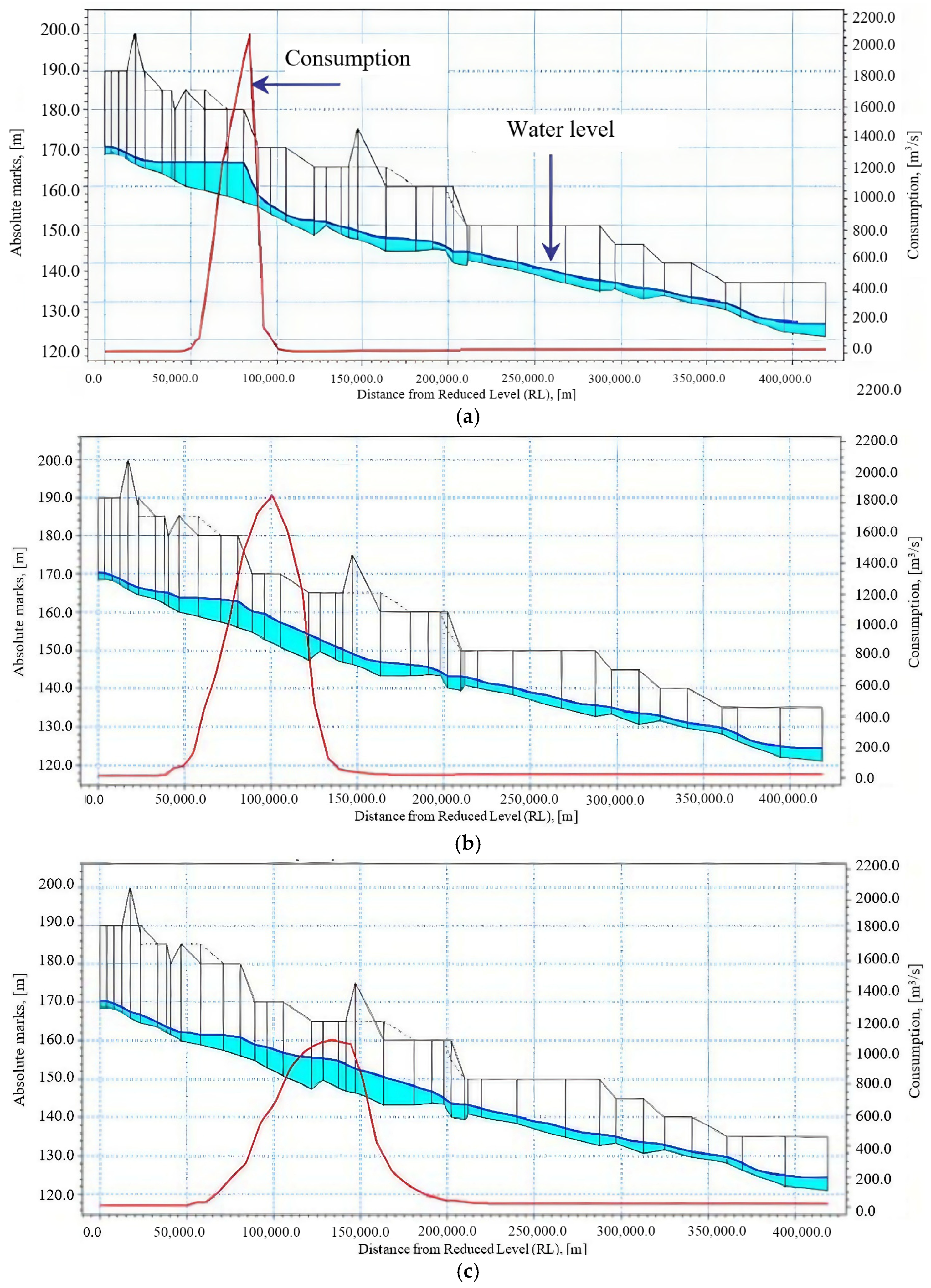
In floods, for river sections of different topologies, it is necessary to model the propagation of a flood wave. The area of maximum wave height (crest) usually moves at a lower speed compared to the wave front (see Figure 3).

Figure 3 shows the sequence of propagation of the outflow wave (flood wave) along the river bed at different points in time. Figure 3a: a sharp peak in flow (~2000 m³/s) is observed at the beginning of the section (about 90–100 km). The maximum water level is observed in the initial zone, then gradually decreases downstream. In Figure 3b, the peak of the outflow wave flow has shifted downstream and has also become less pronounced (~1400 m³/s), demonstrating the transformation of the wave. Water levels continue to decrease, but the zone of maximum rise has also shifted downstream. In Figure 3c, further movement of the wave downstream is observed, the peak flow rate is already lower (~900 m³/s), and the wave shape has smoothed out and decreased significantly. The zone of maximum levels continues to gradually move further downstream, clearly demonstrating the attenuation of the wave. In Figure 3d, the flood wave has weakened significantly (flow rate does not exceed ~400 m³/s). Maximum water levels have noticeably decreased and leveled out, and the distribution of levels has become more uniform. In Figure 3e, the flood wave has almost completely weakened (the flow rate is minimal, less than ~200 m³/s). The water level has almost returned to its original values, and the wave has completed its process of attenuation and transformation. Wave propagation includes various phases, each characterized by changing wave speeds and behaviors. The rear part of the wave, or wave tail, moves more slowly than the crest and the initial wave front. Due to the difference in speeds of these characteristic points, the wave gradually lengthens along the river bed. Accordingly, a decrease in wave height and an increase in its travel time are observed. The lengthening of the wave depends on its height, the slope of the river, the geometry of the channel and floodplain, and the roughness of the river bottom. In some areas, especially where the shape or slope of the channel changes sharply, a temporary acceleration of the wave crest can be observed, which leads to its “skewing” when the rise phase is relatively shorter than the decline phase.

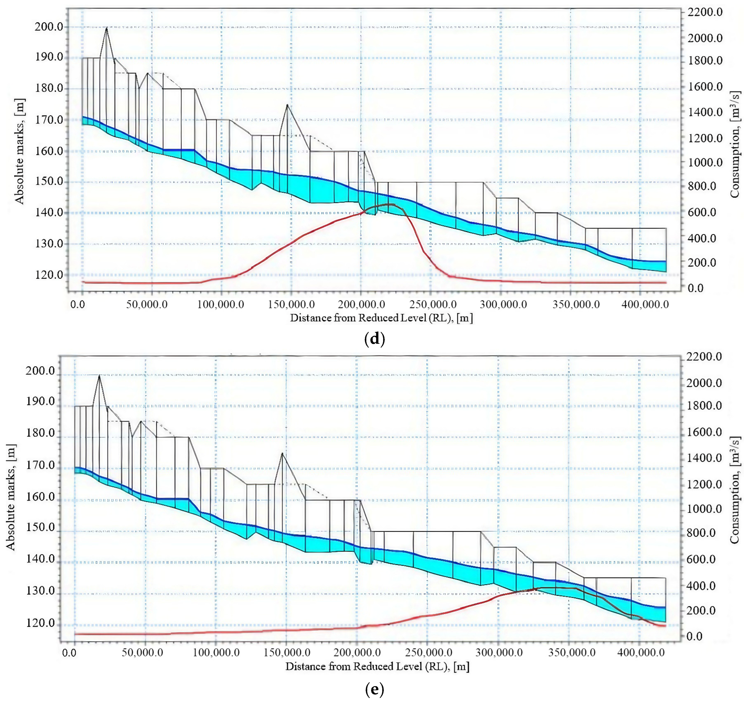
The formation of a flood zone is a key aspect of dam failure events (see Figure 4). As the failure wave moves along the river channel, it continuously changes its height, speed, width, and other parameters. The wave front separating the zones of water level rise and fall may be steep near the failed hydrodynamically hazardous object (HHO) and relatively flat at a considerable distance from it.

The resulting model, using the small Kurchum River as an example, can be used to model and predict the flooding of entire river systems. In early March 2019, an analysis of data on the flood situation in the region was carried out and a preliminary forecast was made about the high probability of flooding in the Beskaragay district. This forecast was confirmed on 28 March 2019, when groundwater levels rose, and settlements in this area were flooded [34]. 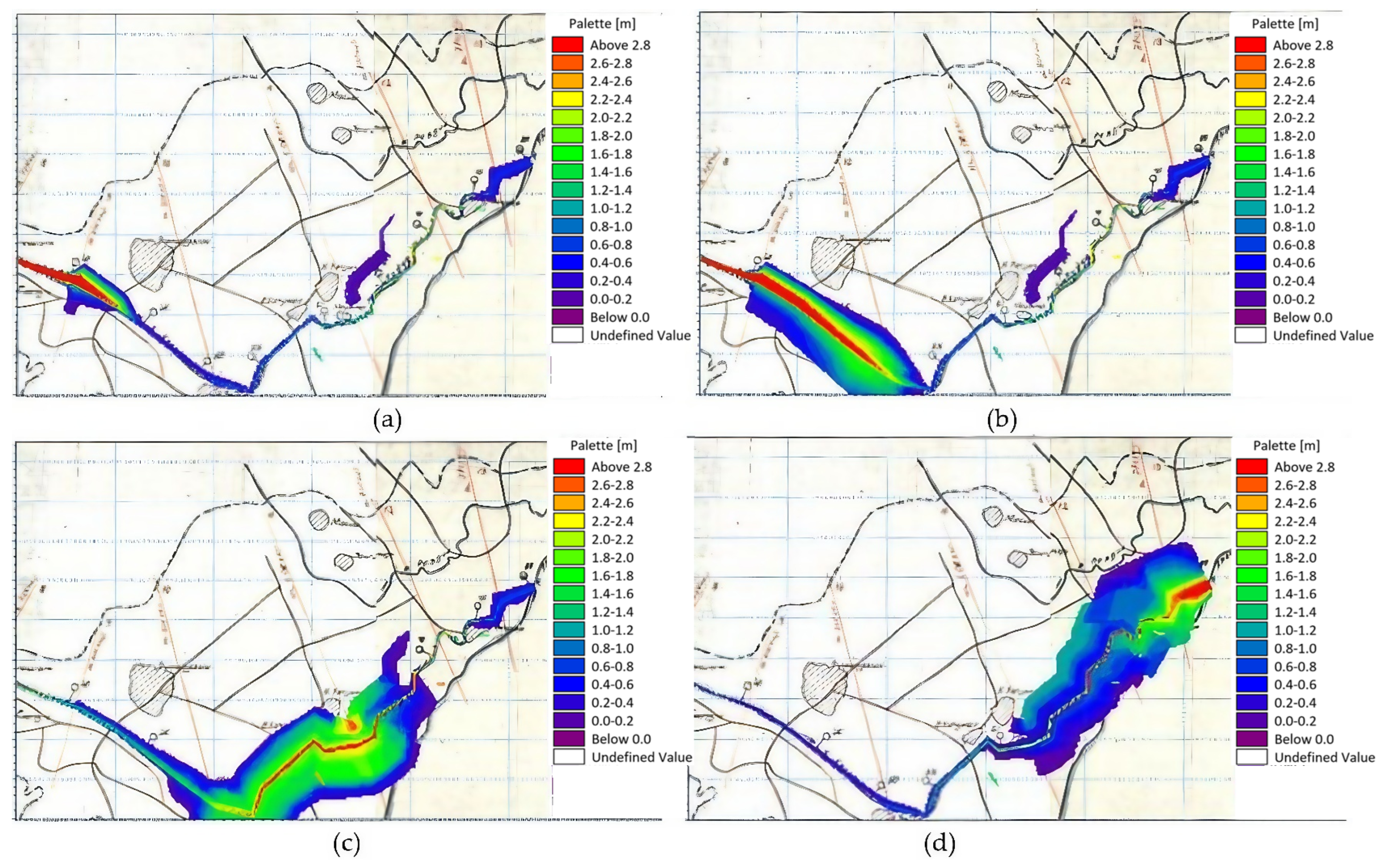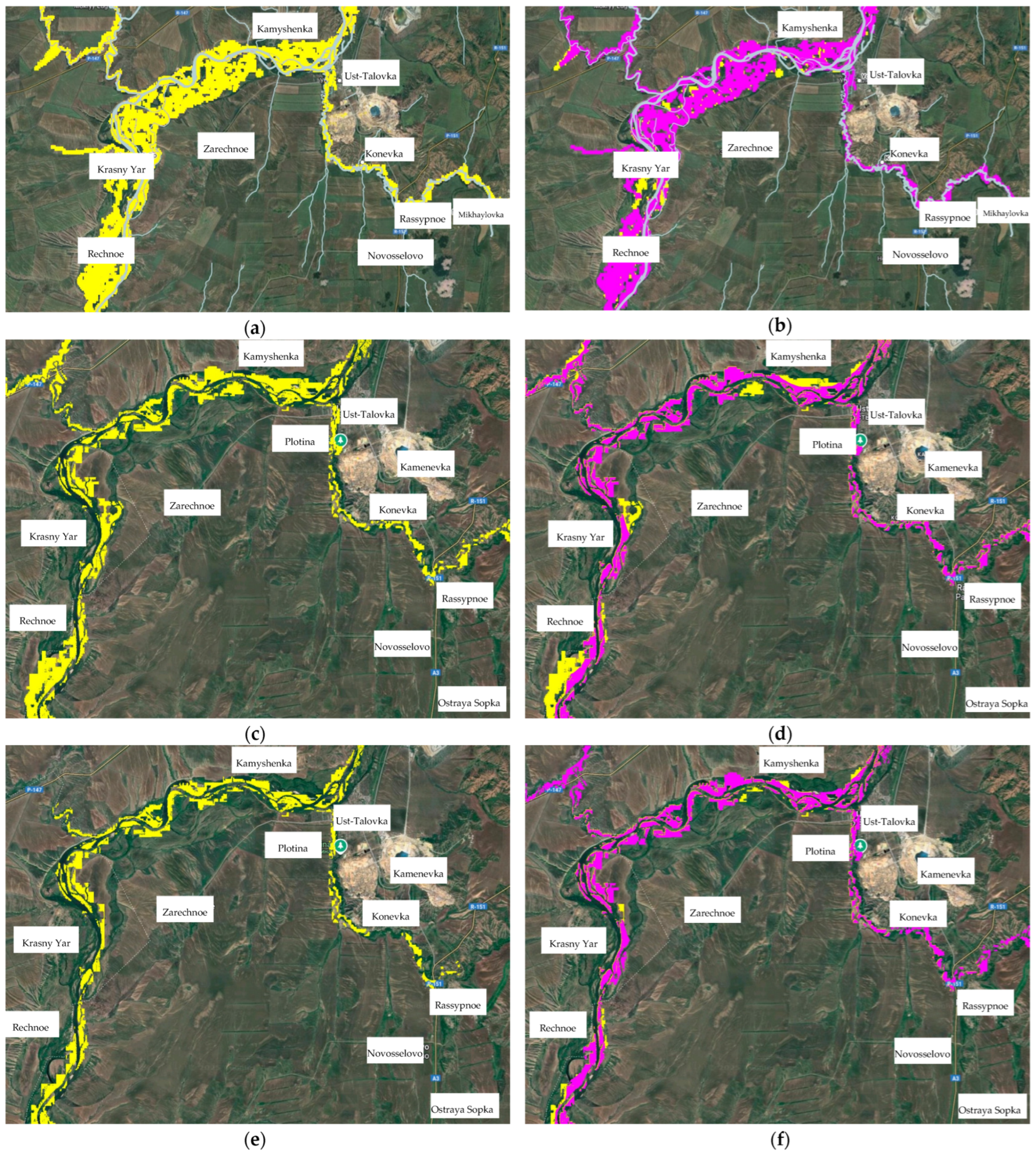Figure 5 shows the results of the analysis of flooding of the territory near settlements in the region, carried out on the basis of actual data and modeling using the analytical system being developed.

Figure 5a shows the actual recorded flood zone based on observations for the period February–March 2019. The yellow areas correspond to the actual areas that were under water as a result of the flood. Figure 5b shows the simulated flood zone calculated using the analytical system. The pink areas superimposed on the yellow ones show intersections, i.e., coincidences between the actual and simulated data.

The degree of coincidence of the simulated flood zones with the actually observed zones was calculated using the methodology described in Section 2 (Materials and Methods), resulting in 91.89% for 2019, 89.09% for 2020, and 95.91% for 2021.

An analysis of the discrepancies between the model simulation results and the actual observed flood extents revealed several potential sources of error that could have influenced the accuracy of the predictions. One of the primary factors is the accuracy and resolution of the digital elevation model (DEM) used in the hydrodynamic simulations. The DEM was derived from Sentinel-2 data with a spatial resolution of up to 10 m and Sentinel-1 data with a resolution of up to 5 m. While these datasets provide high-quality elevation information for regional-scale studies, they may not capture small-scale topographic variations of the floodplain, such as local depressions, levees, or micro-relief features, which can significantly affect the extent of flooding, especially along the boundaries of the flood zones.

Another important source of discrepancy arises from the input hydrological data. The model was forced using streamflow time series from gauging stations at the boundaries, but lateral inflows, local runoff, and contributions from ungauged catchments were not directly measured and could contribute to differences between simulated and observed flood extents. The calibration of hydraulic parameters, such as Manning’s roughness coefficients, was performed based on available data, but the limited number of direct field measurements introduces uncertainty into these parameter values.

In addition, discrepancies may result from the limitations of the observed flood maps themselves. The observed flood extents were derived from satellite imagery, which, despite their high resolution, can be affected by classification errors, such as difficulties distinguishing water surfaces from wet soil or flooded vegetation. These factors can lead to a slight over- or underestimation of actual flooded areas.

Furthermore, it is important to note a temporal limitation of the satellite-based validation approach. The Sentinel-1 satellite acquires data with a fixed revisit interval and may not always capture the peak of a flood event due to a timing misalignment. This latency could lead to an under-representation of the maximum inundation area, especially in fast-evolving flood scenarios. Consequently, even with an accurate spatial resolution, satellite imagery might miss short-lived flood peaks or local maxima, introducing additional uncertainty when compared to the simulated maximum flood extent.

Despite these sources of uncertainty, the high degree of coincidence between the modeled and observed flood extents (greater than 89% for all analyzed events) indicates that the model provides reliable results for flood hazard assessment in the region. Nevertheless, future improvements could include the use of higher-resolution terrain data, enhanced hydrological monitoring of lateral inflows, and more detailed calibration supported by field surveys to further reduce uncertainties.

The accuracy of the model developed in this study, as reflected in the percentage of matching between simulated and observed flood extents (91.89% for 2019, 89.09% for 2020, and 95.91% for 2021), is consistent with or exceeds the results of similar studies conducted in data-limited environments. For example, Szopos et al. (2024) [19] applied hydrodynamic modeling for the Tarna River using HEC-RAS under conditions of limited hydrological data. Their results demonstrate reliable performance for large flood events, with higher accuracy for these larger events as measured by the Kling–Gupta efficiency (KGE) and Nash–Sutcliffe efficiency (NSE). Similarly, in our study, the largest flood event (2021) showed the highest degree of matching, confirming that event magnitude can positively influence model accuracy when appropriate calibration is performed.

Furthermore, Lyu et al. (2024) [11] showed that the use of bias-corrected satellite precipitation data (IMERG V7) improved the accuracy of event-based flood simulations in the Sunshui River Basin. While our study did not directly apply distributed precipitation forcing, the integration of satellite-derived spatial data (Sentinel-1 and Sentinel-2), DEMs, and gauging data provides comparable improvements in model reliability. Our approach aligns with these studies in demonstrating that the integration of diverse and complementary datasets significantly enhances the accuracy of flood hazard models in regions where data availability is limited.

These comparisons reinforce the robustness of our modeling framework and highlight its relevance for flood hazard assessment and management in East Kazakhstan.

Comparative analysis shows that the model generally correctly predicts the main flood zones, especially in the channel part. However, there are discrepancies; in some places, the model overestimates or underestimates the extent of flooding. The developed model was used to forecast floods. The flood hazard monitoring system has been tested since 2021, which is confirmed by open publications in the media [35,36,37].

4. Conclusions

Over the past few decades, the intensive study and analysis of hydrodynamic processes in the East Kazakhstan region have identified key trends and features of river flow behavior. This served as the basis for modeling and forecasting river runoff using the example of the small Kurchum River in the East Kazakhstan region. The resulting model was decomposed into a large river network, and the results were integrated into a flood hazard monitoring system to track, forecast, and respond to floods. This flood hazard monitoring system was integrated into the regional emergency monitoring system, which includes avalanche hazard monitoring [38].

Thus, using retrospective data for 3 years (2019–2021), the small Kurchum River was modeled, and the results obtained were compared with real flood data. The assessment of the forecast model showed that the simulation results coincide with the actual data: 91.89% (2019), 89.09% (2020), and 95.91% (2021). The discrepancy between the actual and model data may be associated with factors such as snow cover conditions, groundwater levels, and input data characteristics (georeferencing accuracy, spatial resolution of images, and digital terrain models), as suggested by the authors’ analysis of data quality and known sources of uncertainty. In addition, the sensitivity of the model is affected by the following factors: the use of high-resolution space images, the use of digital elevation models (DEMs) with a resolution of no more than 5 m, an increase in the number of control hydrological posts, and regular data updates.