KAN-Based Tool Wear Modeling with Adaptive Complexity and Symbolic Interpretability in CNC Turning Processes

Abstract

Tool wear modeling in CNC turning processes is critical for proactive maintenance and process optimization in intelligent manufacturing. However, traditional physics-based models lack adaptability, while machine learning approaches are often limited by poor interpretability. This study develops Kolmogorov–Arnold Networks (KANs) to address the trade-off between accuracy and interpretability in lathe tool wear modeling. Three KAN variants (KAN-A, KAN-B, and KAN-C) with varying complexities are proposed, using feed rate, depth of cut, and cutting speed as input variables to model flank wear. The proposed KAN-based framework generates interpretable mathematical expressions for tool wear, enabling transparent decision-making. To evaluate the performance of KANs, this research systematically compares prediction errors, topological evolutions, and mathematical interpretations of derived symbolic formulas. For benchmarking purposes, MLP-A, MLP-B, and MLP-C models are developed based on the architectures of their KAN counterparts. A comparative analysis between KAN and MLP frameworks is conducted to assess differences in modeling performance, with particular focus on the impact of network depth, width, and parameter configurations. Theoretical analyses, grounded in the Kolmogorov–Arnold representation theorem and Cybenko’s theorem, explain KANs’ ability to approximate complex functions with fewer nodes. The experimental results demonstrate that KANs exhibit two key advantages: (1) superior accuracy with fewer parameters compared to traditional MLPs, and (2) the ability to generate white-box mathematical expressions. Thus, this work bridges the gap between empirical models and black-box machine learning in manufacturing applications. KANs uniquely combine the adaptability of data-driven methods with the interpretability of physics-based models, offering actionable insights for researchers and practitioners.

1. Introduction

Tool wear is an inevitable phenomenon in machining processes [1,2]. Intelligent manufacturing systems require accurate tool wear predictions to optimize production parameters, schedule maintenance activities, and ensure consistent product quality [3]. The phenomenon critically influences product quality, manufacturing efficiency, and operational costs [4,5], with direct economic implications for industry. Unplanned tool failure may lead to increased manufacturing downtime, whereas accurate wear prediction enables just-in-time maintenance strategies that reduce tool replacement costs.

Traditional approaches to tool wear analysis have primarily employed empirical or physics-based models, such as the Usui Adhesion Wear Model and Taylor’s extended formula, which correlate tool life with cutting parameters. Although these classical formulations provide interpretable relationships, their effectiveness is limited by oversimplified assumptions [6]. These limitations reduce their applicability in modern machining scenarios, where dynamic interactions between tools, materials, and processes require more sophisticated modeling frameworks [7]. It is particularly evident in high-mix, low-volume production environments, where tool wear patterns vary significantly across different workpiece materials and cutting conditions. Consequently, traditional models often prove inadequate for real-time adaptive control.

In recent years, machine learning has emerged as a promising alternative for tool wear prediction [8,9,10]. Methods such as neural networks and support vector regression demonstrate superior capability in capturing nonlinear patterns from operational data. Nevertheless, their “black-box” nature presents significant barriers to practical adoption [11]. The lack of interpretability in machine learning models hinders the identification of root causes underlying wear progression [12,13]. Furthermore, these models typically require extensive datasets and computational resources while remaining susceptible to overfitting [14,15]. This situation creates a critical gap between academic research and industrial implementation. Although deep learning models achieve high accuracy in controlled experiments, their deployment in factory settings is frequently impeded by the need for continuous recalibration and the inability to explain decision-making processes to plant engineers.

Unlike conventional machine learning models, Kolmogorov–Arnold Networks (KANs) are a novel class of interpretable neural networks grounded in the Kolmogorov–Arnold representation theorem (KART) [16]. It inherently adopts a “white-box” structure with network layers that are designed as learnable univariate functions [17]. In essence, KANs approximate multivariate functions using an architecture based on KART, bridging the gap between interpretability and accuracy. This dual advantage addresses two major challenges in industrial AI adoption: the need for explainable models in tool condition monitoring and the ability to generalize across different machining scenarios without extensive retraining.

Driven by the need for more interpretable and efficient neural networks, researchers have proposed some KAN variants and tested their effectiveness across diverse problems. For instance, Wang et al. [18] introduced Convolutional Kolmogorov–Arnold Networks (CKANs), combining the foundational principles of KANs with convolutional mechanisms to achieve enhanced interpretability in intrusion detection. Similarly, Aghaei [19] developed the Fractional Kolmogorov–Arnold Network (fKAN), demonstrating the versatility of KANs through the use of adaptive fractional–orthogonal Jacobi functions as basis functions. Reinhardt et al. [20] proposed SineKAN, which substitutes the commonly used B-spline activation functions with re-weighted sinusoidal functions.

The significance of KANs is further evident in computational physics applications. Wang et al. [21] proposed the Kolmogorov–Arnold-Informed Neural Network (KINN) as an alternative to Multi-Layer Perceptrons (MLPs) for solving partial differential equations (PDEs). Similarly, Shuai and Li [22] introduced physics-informed KANs (PIKANs) tailored for power system applications. Additionally, KANs have demonstrated promising results in time-series forecasting. Livieris [23] developed a model known as the C-KAN, which integrates convolutional layers with the KAN architecture to improve multi-step forecasting accuracy.

In image processing, KANs have also garnered attention. Firsov et al. [24] explored KAN-based networks for hyperspectral image classification. Jiang et al. [25] presented the KansNet for detecting pulmonary nodules in CT images. For load forecasting, Danish and Grolinger [26] developed the Kolmogorov–Arnold Recurrent Network (KARN), which integrates KANs with a recurrent neural network (RNN) to improve the modeling of nonlinear relationships in load data. This approach surpasses traditional RNNs in accuracy.

For fault diagnosis, Tang et al. [27] introduced the MCR-KAResNet-TLDAF method, which combines image fusion techniques with KANs to enhance the extraction and recognition of bearing fault features. Likewise, Cabral et al. [28] proposed a KAN-based approach, KAN_Diag, for fault diagnosis in power transformers using dissolved gas analysis. Peng et al. [29] established a method for predicting the pressure and flow rate of flexible electrohydrodynamic pumps using KANs, replacing fixed activation functions with learnable spline-based functions.

In structural analysis, KANs have proven to be a valuable tool. Wang et al. [30] demonstrated KANs’ capability to accurately predict the Poisson’s ratio of a hexagonal lattice elastic network, showing how this ratio transitions with changes in geometric configuration. In environmental science, Saravani et al. [31] evaluated KANs’ performance in predicting chlorophyll-a concentrations in lakes, confirming their robustness in handling nonlinearity and long-term dependencies.

In quantum computing applications, Kundu et al. [32] demonstrated that KANs significantly outperformed MLP-based approaches, achieving higher success probabilities in quantum state preparation. In finance, Liu et al. [33] investigated KAN integration within Finance-Informed Neural Networks (FINNs) to improve financial modeling and regulatory decision-making. For magnetic positioning systems, Gao and Kong [34] developed a KAN-based algorithm, incorporating learnable activation functions through spline functions. Multiple spline curves and strategic thresholds were used to enhance accuracy.

Despite the importance of tool wear in manufacturing processes, research on KANs in this field remains limited. Only two studies had been published by the completion of this work. Bao et al. [35] proposed a novel approach utilizing KANs to map sensor features to real-time maximum flank wear (VBmax), with a Transformer model predicting future wear sequences. Kupczyk et al. [36] employed KANs to predict tool life in gear production from carburizing alloy steels, demonstrating accurate predictions based on cutting speed, coating thickness, and feed rate.

The unique advantages of KANs for tool wear modeling include the following: (1) a mathematical foundation that enables rigorous error bound analysis, ensuring prediction reliability for safety-critical manufacturing operations; (2) an adaptive basis function selection mechanism that reduces model complexity compared to conventional neural networks, facilitating deployment on resource-constrained edge devices; and (3) interpretable mathematical expressions generated by KANs that provide actionable insights for process optimization.

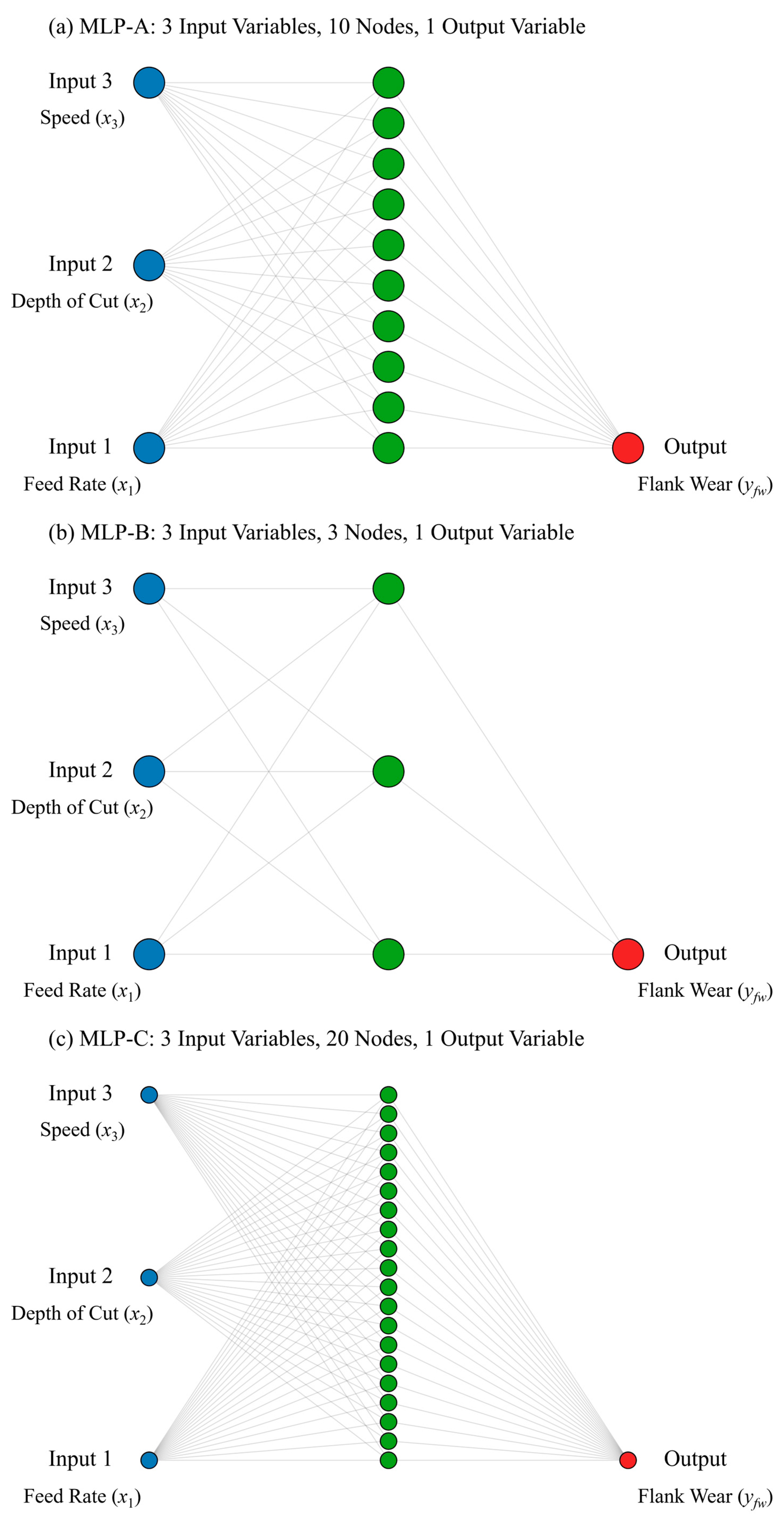
This study proposes three KAN-based models to address tool wear modeling in CNC turning processes. First, KAN-A, KAN-B, and KAN-C models with progressively increasing complexity are developed, accompanied by detailed training protocols and parameter specifications. The readily measurable cutting parameters (feed rate, depth of cut, and cutting speed) are adopted as independent variables. Mathematical expressions relating these variables to flank wear are established using the KAN-A, KAN-B, and KAN-C models, respectively. Furthermore, the physical interpretability of the derived formulas is systematically analyzed from three complementary perspectives: (1) a variable importance assessment, (2) the topological evolution of KAN architectures, and (3) the mathematical relationships between input–output variables. A comparative analysis of KAN-A, KAN-B, and KAN-C is conducted to evaluate modeling errors and identify their underlying causes. Subsequently, MLP-A, MLP-B, and MLP-C models are designed by referencing the topological structures of their KAN counterparts. A comparative study between KAN and MLP frameworks is performed to examine differences in tool wear modeling performance. Particular emphasis is placed on analyzing the effects of network depth, width, and parameter configurations, which reveals distinct sensitivities to architectural variations. The fundamental disparities in modeling capabilities are theoretically interpreted through the lens of KART and Cybenko’s Theorem. Finally, this work systematically compares classical wear equations, machine learning methods, and KAN-based approaches, highlighting their respective strengths. Simulations of turning processes are conducted using DEFORM-3D to further evaluate the wear modeling capabilities of KAN-A, KAN-B, and KAN-C. The advantages of the KAN-derived formula, along with its applicability and limitations, are thoroughly discussed.

The remaining parts of this paper are organized as follows: Section 2 presents the fundamental principles of KANs and the architectures of the proposed models. In Section 3, the public dataset is described, and three modeling experiments are conducted. Additionally, the mathematical expressions derived from KANs and their physical interpretations are discussed. Section 4 introduces multiple metrics to quantify modeling errors and computational efficiency. A vertical comparison of modeling performance among KAN-A/B/C is performed, with a systematic evaluation of error analysis and performance trade-offs. In Section 5, three MLP-based neural networks are constructed, mirroring the configurations of KAN-A/B/C, respectively. A horizontal pairwise comparison of prediction errors is presented. The underlying causes of performance disparities are analyzed through the theoretical frameworks of KART and Cybenko’s theorem. Section 6 provides a comparative analysis of classical tool wear equations, machine learning methods, and KAN-based approaches. Section 7 simulates turning operations and employs KAN-A/B/C for tool wear modeling, discussing both the advantages and limitations of the approach. Finally, the research findings are synthesized to form a comprehensive conclusion, and potential future research directions are outlined.

2. Principles and Model Architecture of KANs

2.1. Fundamental Principles

Kolmogorov–Arnold Networks (KANs) are neural architectures grounded in the Kolmogorov–Arnold representation theorem, which asserts that any multivariate continuous function can be decomposed into a finite composition of univariate functions and additive operations. Unlike conventional Multilayer Perceptrons (MLPs) that employ fixed nonlinear activation functions at nodes, KANs parameterize learnable activation functions on edges. They offer enhanced interpretability and flexibility.

KART offers a theoretical foundation for expressing a high-dimensional function f(x) as a superposition of univariate functions, as shown in Formula (1). ${\varphi }_{q,p}$ and ${\Phi }_q$ are univariate functions. KANs operationalize this by structuring networks to learn these inner and outer functions adaptively.

Edges (rather than nodes) hold trainable activation functions. They are typically parameterized via B-splines. Nodes aggregate inputs linearly, while edges apply nonlinear transformations. The inversion of roles compared to MLPs enables fine-grained control over function approximation.

Activation functions on edges are represented as linear combinations of basis functions (B-splines) with learnable coefficients. For an edge connecting node i to j, the activation is shown in Formula (2).

$$f(\mathit{x})=\sum _{q=1}^{2n+1}{\Phi }_q\left(\sum _{p=1}^n{\varphi }_{q,p}(x_p)\right)$$

(1)

$${\sigma }_{ij}(x)=\sum _k{c}_{ijk}\cdot B_k(x)$$

(2)

where B_k are basis functions and c_ijk are trainable parameters. It allows the KANs to dynamically adjust activation shapes during training. KANs often use grid structures to discretize the input domain of basis functions. The gradients are computed via automatic differentiation. The parameters are optimized using gradient descent with regularization to improve smoothness and prevent overfitting.

2.2. Model Structure and Parameter Configuration

Three initial KAN structures were designed for modeling, respectively, with their configurations listed in

Table 1. Three initial KAN structures.

Name	KAN-A	KAN-B	KAN-C
Each Layer of KAN	1 output variable 10 nodes 3 input variables	1 output variable 3 nodes 3 input variables	1 output variable 20 nodes 3 input variables
Total Number of Nodes	3 + 10 + 1 = 14	3 + 3 + 1 = 7	3 + 20 + 1 = 24

. A training protocol for KANs is proposed, accompanied by corresponding parameter specifications, as shown in

Table 2. KAN training protocols and parameters.

Number	Training Stage	Procedures and Parameter Setting
1	Network Structure Setup	Grid structure configuration: grid size set to 8, k B-spline order set to 5
2	First Training	Optimization algorithm: LBFGS Number of iterations (steps): 500 Regularization coefficient (λ): 0.01
3	Model Pruning	Node attribution score threshold (node_th): 2 × 10−2 Edge attribution score threshold (edge_th): 2 × 10−2
4	Second Training	Optimization algorithm: LBFGS Number of iterations (steps): 500 Regularization coefficient (λ): 0
5	Symbolic KAN Conversion	R2 threshold for goodness-of-fit: 0.7 Preference weight for model simplicity (weight_simple): 0.5
6	Third Training	Optimization algorithm: LBFGS Number of iterations (steps): 300 Regularization coefficient (λ): 0
7	Output and Calculation	Output symbolic expressions with 1-digit and 2-digit decimal precision sequentially Calculate errors of KAN on training and test datasets

.

Different from classical artificial neural networks, the connection patterns between layers of KANs evolve dynamically during training. In this study, the KAN structure immediately after loading the training dataset is defined as the initial structure. After completing the first training phase, the inter-layer connection patterns typically undergo changes, resulting in the post-training structure. The structure formed after model pruning is termed the pruned structure, which is generally much simpler than the previous two structures due to the removal of redundant network nodes and connecting edges.

3. Public Data and Modeling Experiments

3.1. Public Data Description

The dataset is obtained from Kaggle (accessible at https://www.kaggle.com/datasets/drganeshkumars/flank-wear-of-cnc-lathe-tool-insert-dataset, accessed on 17 January 2025), documenting the flank wear of CNC lathe tool inserts. The preprocessed dataset can also be directly accessed via this URL (accessed on 10 May 2025): https://github.com/567ZYC/Data-Processing-and-Explanation-for-Flank-Wear-of-CNC-Lathe-Tool-Insert-Dataset-.

Flank wear, a detrimental phenomenon in single-point cutting processes, arises from adhesion and abrasion when the cutting tool contacts the workpiece. It is measured by distinguishing geometric relationships in rake face images between new and worn tools.

Flank wear of lathe tools impacts machining quality: it degrades surface finish, increases tool replacement frequency, reduces machining efficiency, and may cause dimensional errors affecting overall precision. Tool wear is primarily influenced by the feed rate, depth of cut, and cutting speed during turning, as summarized in

Table 3. Key factors influencing flank wear of lathe tools.

Category	Physical Variable	Symbol	Description
Input	Feed rate	fr	Distance the tool travels per unit time along the machining direction, affecting machining efficiency and surface roughness.
	Depth of cut	dec	Vertical thickness of material penetrated by the tool in a single pass, determining material removal volume and directly correlating with cutting force.
	Speed	sp	Linear velocity at the contact point between the tool edge and workpiece, characterizing friction and heat generation intensity during cutting.
Target	Flank wear	fw	Material loss on the tool flank due to friction with the workpiece, impacting machining precision and surface quality of parts.

. Establishing mathematical relationships between these physical variables and flank wear serves as the foundation for intelligent optimization of cutting parameters.

The dataset contains 2001 samples without missing values. However, 45 samples were incorrectly recorded as negative or excessively large values (physically meaningless for flank wear measurement) and were thus removed, leaving 1956 samples for experiments. The training and test sets were divided at a 1:1 ratio.

3.2. Modeling Experiment Based on KAN-A

First, experiments using KAN-A for training and modeling were conducted. Figure 1 illustrates three structural states of KAN-A and their evolutions during training. Guided by mathematical priors from KART, simple basis functions with uniform distributions are typically used during initialization. The initial structure has dense but redundant connections. The parameters remain unadopted to data distributions. It is analogous to an “uncarved blank”.

The post-training structure exhibits substantial differences from the initial structure: the waveform of the activation function (B-spline) adjusts its shape after one training cycle, becoming either more peaked or smoother depending on data characteristics and training parameters. Concurrently, these dynamic adjustments optimize the positions and coefficients of the B-spline control points. Some connection weights are significantly strengthened, while others approach zero. It is a data-driven feature selection process.

Pruning endows KANs with a more compact topology by retaining task-sensitive B-spline functions and removing less relevant ones. The pruned structure, free of redundant nodes and edges, serves as the basis for symbolic computation of KANs. Notably, in the initial structure, the third input variable was connected to all nodes. The first two input variables had no connections. This was due to dimensional discrepancies between the variables. During initialization, the first two variables exhibited lower gradient magnitudes, leading to misjudgments of their importance. However, after training and pruning, their importance was significantly enhanced. It indicates that the KAN’s initial structure does not necessarily reflect true feature significance. Instead, the training process involves learning the importance of input variables. Thus, it can be inferred that KANs have the ability to automatically select core features.

Mathematical relationships between the input variables (feed rate, depth of cut, and speed) and the output variable (flank wear) were derived via the KAN. Formulas with coefficients retained to 1, 2, and 4 decimal places are provided, as follows:

$$y_{fw}=0.1\left|9.8x_1-3.2\right|-0.5\sin (0.6x_2+2.2)-0.62$$

(3)

$$y_{fw}=-0.5\sin \left(0.61x_2+2.19\right)+0.14\left|9.81x_1-3.22\right|-0.05\left|0.02x_3-5.5\right|-0.1$$

(4)

$$\begin{array}{l}{y}_{fw}=0.0011x_3-0.495\sin \left(0.6052x_2+2.1927\right)+0.1438\left|9.815x_1-3.2184\right|\\ -0.053\left|0.0213x_3-5.5006\right|-0.103\end{array}$$

(5)

A higher coefficient precision can enhance modeling accuracy, but it might also bring in noise due to the retention of some negligible terms. Lower-precision formulas facilitate clearer interpretation of mathematical connections between inputs and outputs. Taking Formula (3) as an example, the effects of the feed rate (x₁), depth of cut (x₂), and speed (x₃) on flank wear (y_fw) are discussed.

The physical meaning of $0.1\left|9.8x_1-3.2\right|$ is that when $9.8x_1=3.2$, the relationship between the feed rate and flank wear undergoes a sudden change. At lower feed rates, flank wear decreases linearly with an increasing feed rate, possibly due to insufficient cutting force prolonging tool–material friction time, where frictional effects dominate tool wear. Conversely, at higher feed rates, flank wear increases linearly with the feed rate. Sharp increases in cutting force elevate mechanical stress and thermal load on the tool. Consequently, the tool wear is accelerated.

Unlike the feed rate (x₁), the second term $-0.5\mathit{sin}(0.6x_2+2.2)$ in the formula indicates that flank wear fluctuates periodically with the depth of cut. It may arise from periodic changes in tool force distribution caused by varying cutting depths. Due to the phase shift of the sine function, as the depth of cut increases, flank wear first decreases and then increases overall. It is hypothesized that specific cutting depths may correspond to the tool’s resonance frequency, exacerbating wear; at other depths, stress dispersion or non-resonant conditions lead to less severe wear.

Speed (x₃) does not explicitly appear in the formula for two reasons: firstly, KANs’ pruning process removed the speed-related connections deemed insignificant to the output. Secondly, terms with x₃ as the coefficients were too small to contribute to the flank wear modeling, and were thus eliminated when retaining 1-digit decimal precision.

Compared with machine learning and deep learning approaches, KAN-based symbolic modeling not only clarifies mathematical relationships between variables (as a white-box model) but also provides precise guidance for machining process optimization. For example, to minimize flank wear, the feed rate (x₁) and depth of cut (x₂) can be configured based on $0.1\left|9.8x_1-3.2\right|$ and $-0.5\mathit{sin}(0.6x_2+2.2)$, while the speed (x₃) can be determined according to roughing or finishing requirements.

This advantage is generalizable: the established mathematical relationships adapt to different datasets. For researchers, changes in physical relationships become focal points of discussion. For engineers, mathematical connections between variables under diverse machining demands and conditions can be obtained to optimize processes toward specific goals. It transcends reliance on empirical intuition.

3.3. Modeling Experiment Based on KAN-B

KANs’ learning capability does not correlate positively with the number of network nodes or layers. KART states that any multivariate continuous function can be decomposed into a combination of finite univariate functions.

KANs can directly learn to approximate these functions efficiently. This reduces dependence on network depth. Therefore, KAN-B was designed as a KAN with an extremely simple structure. Its purpose was to investigate KAN characteristics through analysis of its test results. We aimed to analyze the similarities and differences between the mathematical relationships of KAN-B and those of KAN-A.

Most parameters of KAN-B are consistent with KAN-A, with modified parameters listed in

Table 4. KAN-B training protocols and parameters.

Number	Training Stage	Procedures and Parameter Settings
1	Model Pruning	Node attribution score threshold (node_th): 1 × 10−2 Edge attribution score threshold (edge_th): 1 × 10−2
2	Second Training	Optimization algorithm: LBFGS Number of iterations (steps): 300 Regularization coefficient (λ): 0
3	Symbolic KAN Conversion	R2 threshold for goodness-of-fit: 0.4 Preference weight for model simplicity (weight_simple): 0.2

.

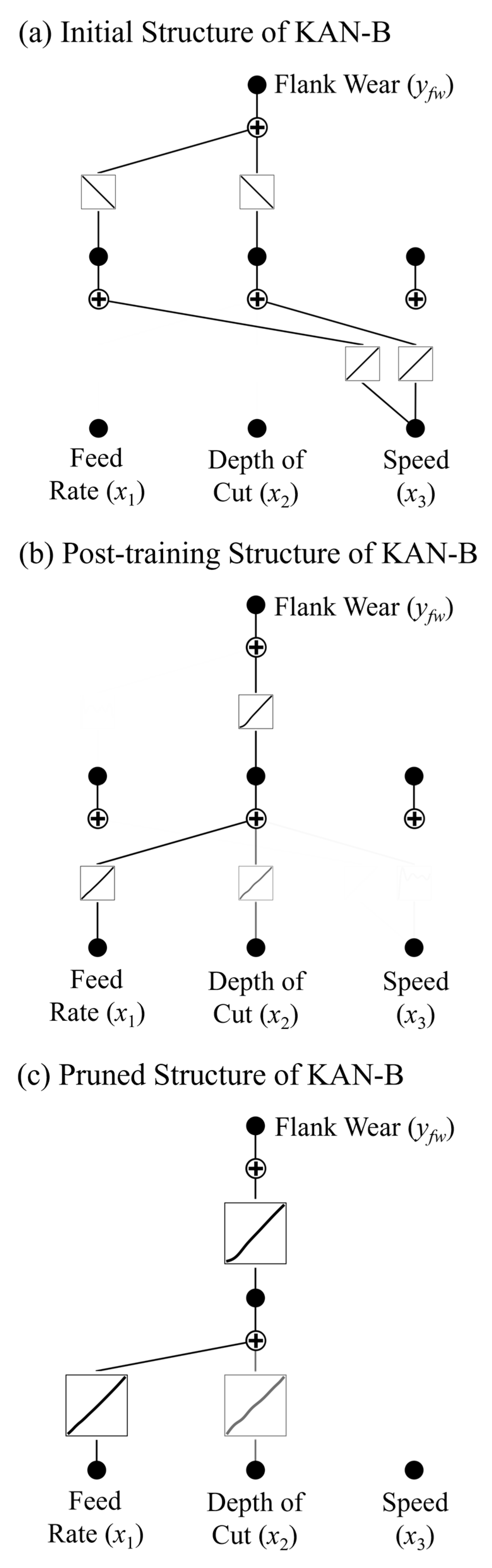
The initial, post-training, and pruned structures of KAN-B are shown in Figure 2. After first loading the training data, KAN-B identified speed (x₃) as the most important variable, again influenced by data dimensionality. After training, the increased weights of the feed rate (x₁) and depth of cut (x₂) demonstrate that the sparse connections from the input layer to the first hidden layer prioritize these two features. After pruning, the nodes and edges of low modeling importance were removed, which makes the relationship between input vectors and output targets intuitive.

Mathematical relationships between the input variables (feed rate, depth of cut, and speed) and the output variable (flank wear) were derived based on KAN-B. The formulas with coefficients retained to 1, 2, and 4 decimal places are provided, as follows:

$$y_{fw}=0.1\left|10.7x_1+2.2x_2-6.0\right|$$

(6)

$$y_{fw}=0.13\left|10.72x_1+2.23x_2-5.98\right|+0.04$$

(7)

$$y_{fw}=0.1324\left|10.7228x_1+2.2276x_2-5.9784\right|+0.0438$$

(8)

Formula (6) highlights a core term: $\left|10.7x_1+2.2x_2-6.0\right|$. The absolute value describes wear asymmetry: wear accelerates when the linear combination exceeds the threshold, while the wear rate remains lower below the threshold. The coefficient 0.1 before the absolute value acts as a scaling factor. The linear terms $10.7x_1$ and $2.2x_2$ indicate that the feed rate (x₁) contributes more to wear than the depth of cut (x₂).

Speed (x₃) does not appear in the formula, suggesting that within the experimental parameter range, its impact on flank wear is insignificant. The constant term −6.0 represents a critical threshold: when $10.7x_1+2.2x_2>6.0$, the wear begins to increase. This constant may relate to turning conditions or material properties.

Formula (6) shares similarities with Formula (3): both reflect a threshold effect in wear, where wear increases notably when variables exceed specific limits, and neither includes terms for speed (x₃). However, Formula (3) contains a sine term, which better describes wear fluctuations. The more complex structure of KAN-A, with a larger number of nodes, facilitates fitting more intricate mathematical relationships.

3.4. Modeling Experiment Based on KAN-C

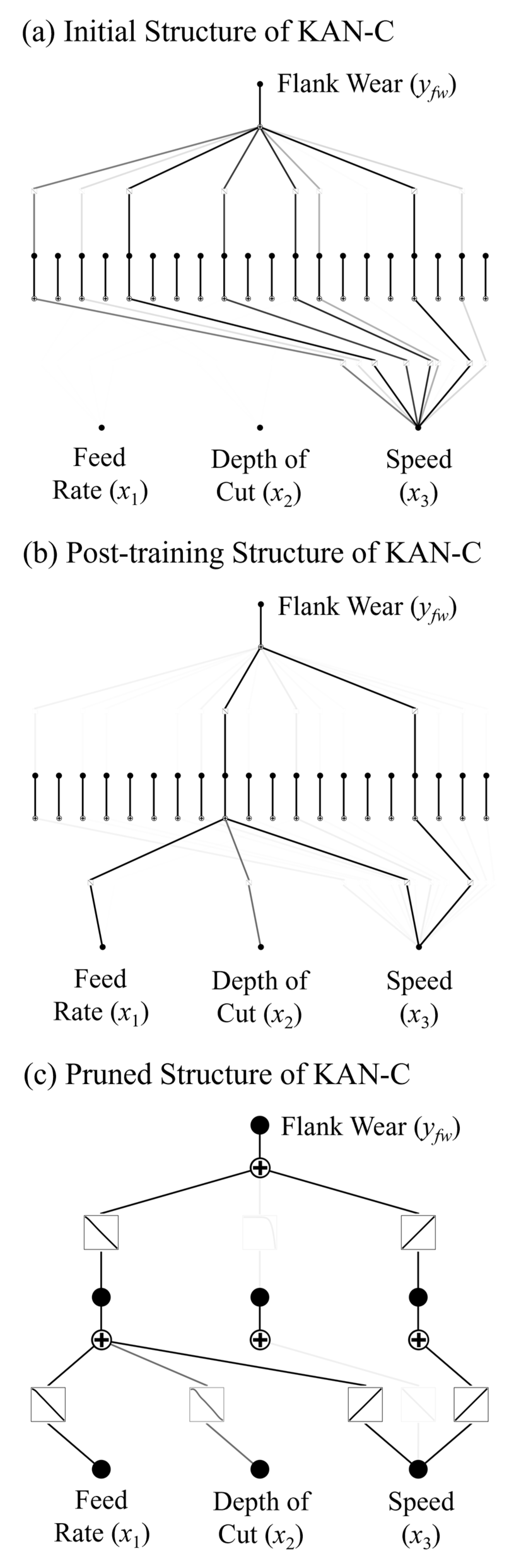
KAN-C, featuring the largest number of neural nodes, offers greater degrees of freedom in modeling input–output relationships compared to KAN-A and KAN-B. Figure 3 illustrates its three network structures.

The initial structure displays the neurons and connections in KAN-C. The post-training structure shows dynamic parameter adjustments, such as reduced weights (observed as lighter colors) for some neurons and connections and strengthened weights for frequently activated neurons (observed as darker colors). Despite its complex initial structure, numerous nodes and edges were pruned away in the final pruned structure.

Similar to KAN-A and KAN-B, KAN-C retains KANs’ common characteristics: upon data loading, input features with larger numerical values were deemed more important. After training and pruning, information transmission in KAN-C shifted to prioritize the feed rate (x₁) and depth of cut (x₂) as primary features.

Mathematical relationships between the input variables (feed rate, depth of cut, and speed) and the output variable (flank wear) were established using KAN-C. Formulas with coefficients retained to 1, 2, and 4 decimal places are provided, as follows:

$$y_{fw}=0.3x_2+0.2\left|6.9x_1-2.2\right|-0.2$$

(9)

$$y_{fw}=0.29x_2+0.21\left|6.89x_1-2.23\right|-0.29$$

(10)

$$y_{fw}=0.2877x_2+0.2058\left|6.8862x_1-2.2267\right|-0.1393-0.1451e^{-0.0004x_3}$$

(11)

The piecewise linear structure of Formula (9) aligns well with the general physical characteristics of tool wear, where wear rates often exhibit abrupt changes as process parameters exceed critical thresholds in practical machining. First, focusing on its linear term: $0.3x_2$ indicates a positive correlation between the depth of cut (x₂) and flank wear (y_fw), with the coefficient 0.3 quantifying the intensity of this effect.

The nonlinear term $0.2\left|6.9x_1-2.2\right|$ reveals a critical effect of the feed rate (x₁). The turning point occurs when 6.9x₁ = 2.2, where the impact of the feed rate on wear is minimized. The presence of the absolute value function validates KANs’ capability to automatically identify nonlinear features. Speed (x₃) does not appear in the formula, indicating its contribution is lower than other features in this dataset. An alternative possibility is that x₃ implicitly influences other parameters, thereby affecting flank wear (y_fw).

Furthermore, Formula (9) contains both linear and absolute value terms, showing similarities with Formulas (3) and (6). KAN-A, KAN-B, and KAN-C exhibit commonalities in structure, training processes, and modeling results. This demonstrates that KANs’ modeling of physical processes is less susceptible to network design and possesses generalizability.

4. Modeling Errors of KANs and Discussion

4.1. Error Metrics

Multiple error metrics were selected, including the Mean Squared Error (MSE), Mean Absolute Error (MAE), Symmetric Mean Absolute Percentage Error (sMAPE), MaxAE (Maximum Absolute Error), Coefficient of Determination (R²), and Adjusted R². Their mathematical formulas are defined as:

$$MSE={\displaystyle \frac{1}{n}}\sum _{i=1}^n{(y_i-{\widehat{y}}_i)}^2$$

(12)

$$MAE={\displaystyle \frac{1}{n}}\sum _{i=1}^n|y_i-{\widehat{y}}_i|$$

(13)

$$sMAPE={\displaystyle \frac{100\%}{n}}\sum _{i=1}^n{\displaystyle \frac{|y_i-{\widehat{y}}_i|}{(|y_i|+|{\widehat{y}}_i|)/2}}$$

(14)

$$MaxAE=\max (|y_i-{\widehat{y}}_i|)\hspace{1em}(i=1,\mathrm{\dots },n)$$

(15)

$$R^2=1-{\displaystyle \frac{S{S}_{res}}{S{S}_{tot}}}=1-{\displaystyle \frac{\sum {(y_i-{\widehat{y}}_i)}^2}{\sum {(y_i-\overline{y})}^2}}$$

(16)

$$R_{adju}^2=1-{\displaystyle \frac{(1-R^2)(n-1)}{n-p-1}}$$

(17)

where $y_i$ is the actual observed value, ${\widehat{y}}_i$ is the predicted value, n is the total number of samples, $S{S}_{res}$ represents the sum of the Squared Residuals, $S{S}_{tot}$ represents the total Sum of Squares, and p is the number of independent variables.

The MSE is sensitive to outliers due to squared errors, penalizing large deviations strongly. The MAE offers robustness against outliers and reflects overall performance on training and test sets. Unlike the MAPE, the sMAPE stabilizes near-zero values with a fixed range (0–200%), enabling better model comparability. The MaxAE captures the worst-case performance, while R² and Adjusted R² jointly prevent overfitting misjudgment by accounting for variable quantity.

4.2. Modeling Errors of KAN-A

Table 5. Modeling errors of KAN-A.

Model	Category	Error	Value
KAN-A	Training	MSE	0.0019
		MAE	0.0108
		sMAPE	5.4526
		MaxAE	0.7555
		R2	0.9949
		Adjusted R2	0.9949
	Test	MSE	0.0007
		MAE	0.0099
		sMAPE	4.6164
		MaxAE	0.3350
		R2	0.9983
		Adjusted R2	0.9983
	Total runtime		614.5063 s

presents the experimental results for KAN-A. KAN-A’s test set errors (MSE, MAE, and sMAPE) were marginally lower than the training set values, validating the regularization strategy’s effectiveness and demonstrating generalization. The MaxAE decreased from 0.7555 (training) to 0.3350 (test), which suggests improved prediction of extreme cases.

Both R² and Adjusted R² approached 1, confirming that KAN-A explained most variance between the inputs and outputs. The model not only learned data patterns but also generalized them effectively.

The total runtime for KAN-A was 614.5063 s. This duration is substantial but justified by its symbolic output. Once validated with low errors, the derived mathematical relationships will directly guide research and engineering efforts. There is no need for retraining, which makes it cost-efficient in the long term.

4.3. Modeling Errors of KAN-B

The results of KAN-B appear in

Table 6. Modeling errors of KAN-B.

Model	Category	Error	Value
KAN-B	Training	MSE	0.0004
		MAE	0.0018
		sMAPE	1.4544
		MaxAE	0.4950
		R2	0.9990
		Adjusted R2	0.9990
	Test	MSE	0.0004
		MAE	0.0020
		sMAPE	1.9151
		MaxAE	0.4736
		R2	0.9988
		Adjusted R2	0.9988
	Total runtime		299.5320 s

. KAN-B exhibited minimal discrepancies between training and test errors, indicating no overfitting/underfitting. The sMAPE values demonstrated tight control over relative errors. The MaxAE values (0.4950 training, 0.4736 test) showed robust fitting of challenging samples. With a runtime of ~300 s (half of KAN-A), its simple structure delivered computational efficiency.

R² and Adjusted R² remained near 1, confirming that KAN-B fully explained target variance and statistically input contributions. This implies that KAN-B learned universal underlying patterns in the data. The derived mathematical expressions are valid and trustworthy.

4.4. Modeling Errors of KAN-C

The experimental results of KAN-C are shown in

Table 7. Modeling errors of KAN-C.

Model	Category	Error	Value
KAN-C	Training	MSE	0.0005
		MAE	0.0062
		sMAPE	4.0589
		MaxAE	0.3513
		R2	0.9986
		Adjusted R2	0.9986
	Test	MSE	0.0020
		MAE	0.0079
		sMAPE	3.7965
		MaxAE	0.7884
		R2	0.9947
		Adjusted R2	0.9947
	Total runtime		747.6609 s

. Its R² and Adjusted R² on the training set both reach 0.9986, which indicates excellent fitting performance for the training data. Although slightly lower, the R² and Adjusted R² of the test set remain close to 0.9950, demonstrating good generalization capability.

The MaxAE of the test set is roughly double that of the training set, indicating larger maximum prediction errors in testing. The gap explains why KAN-C performs better on training data than on test data. The MSE and MAE metrics follow this pattern consistently.

However, the test set’s sMAPE (3.7965) is smaller than the training set’s (4.0589). This may be attributed to the larger overall magnitude of flank wear in the test set: according to the sMAPE formula, relative errors are diluted when actual values increase, leading to a numerically smaller sMAPE.

4.5. Vertical (Intra-Method) Comparisons of Modeling Results Among KAN-A/B/C

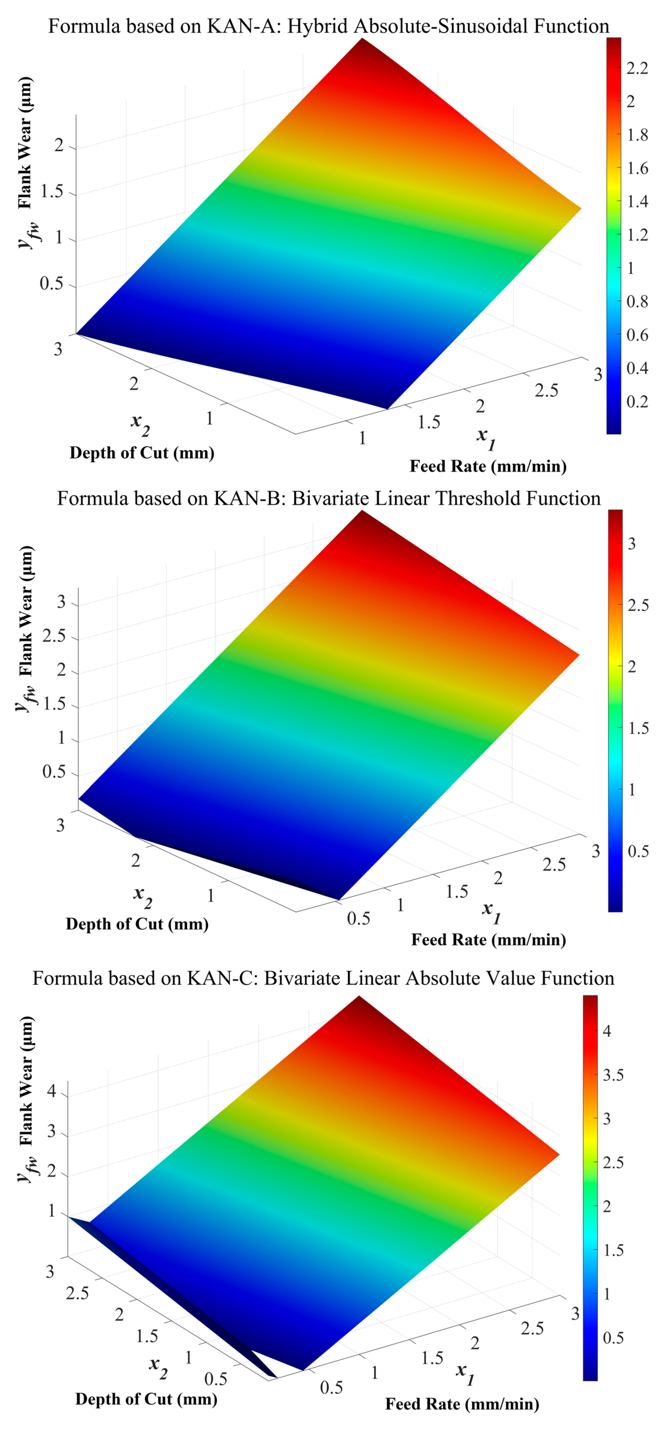
Three-dimensional plots of Formulas (3), (6), and (9) are presented in Figure 4. Flank wear physically cannot be negative. When x₁ and x₂ take small values, both KAN-A and KAN-B predict negative flank wear, while KAN-C only exhibits a small region of negative predictions.

This indicates that KANs’ symbolic conversion process lacks the constraints of physical knowledge. In other words, it currently cannot interpret variable meanings or relationships, and instead only obtains “white-box” mathematical expressions between the input features and the output targets through fitting with minimized errors and pruning. Nevertheless, KANs represent an advancement in artificial intelligence interpretability compared to numerous “black-box” models.

Comparisons among the three plots also reveal an insight: KANs’ learning process and symbolic formulas are constrained by data characteristics. The final expression forms depend on the dataset scale, dimensionality, and value ranges. Although KAN-A/B/C have distinct architectures in this study, their functional forms exhibit substantial commonalities due to using the same dataset.

The effective application range of mathematical formulas derived by KANs is also dataset-dependent. For example, if an input variable’s sample range during training is [0.5, 20], the formula’s validity most likely remains within [0.5, 20]. KANs cannot guarantee the accurate description of input–output relationships outside the range.

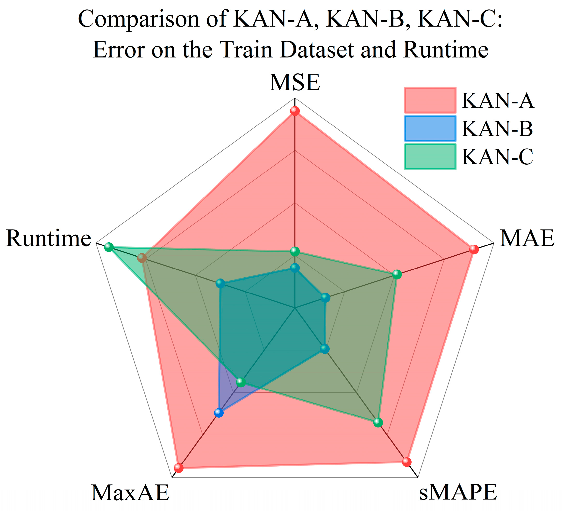
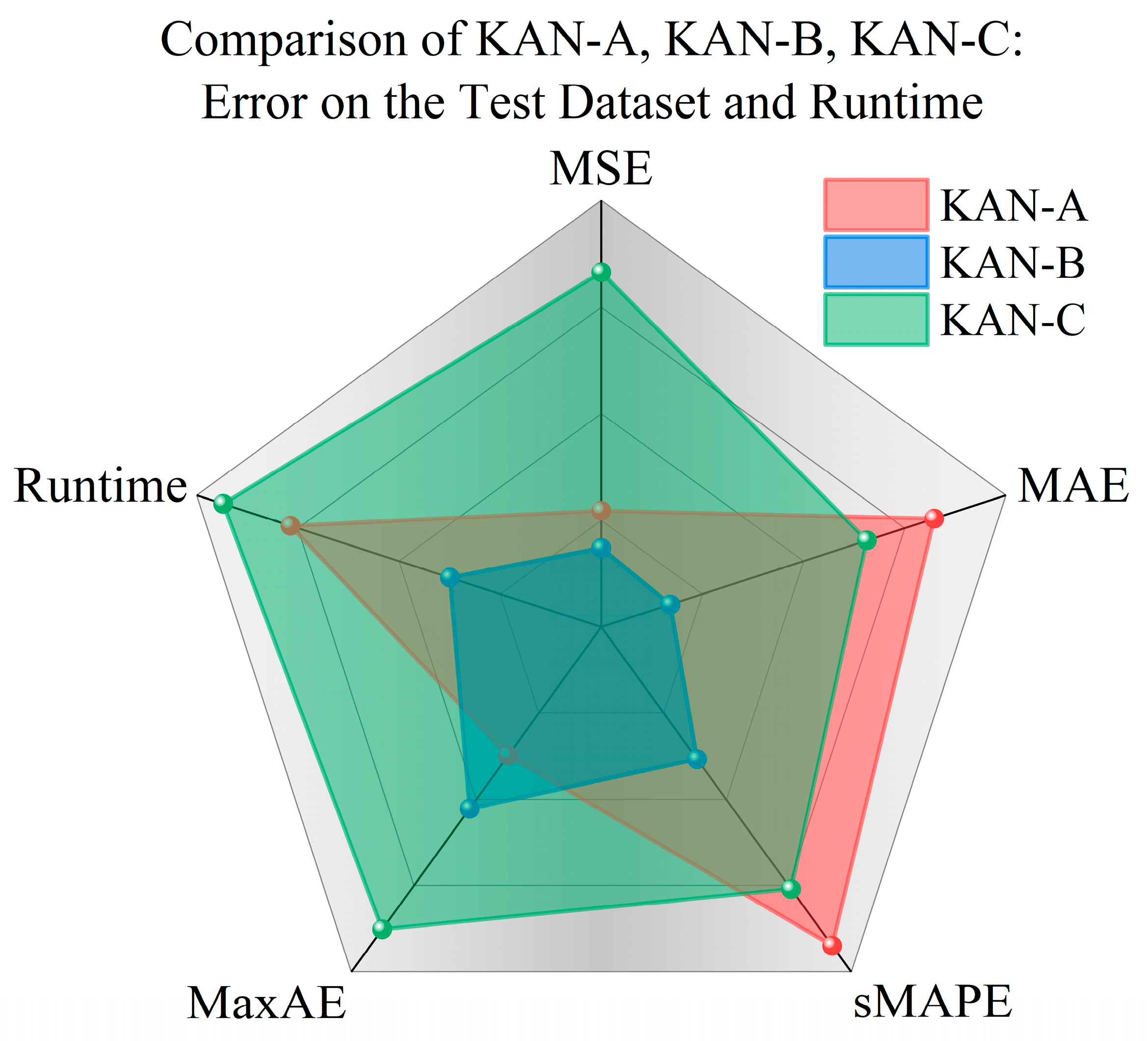
Radar charts plotting the total runtime and error metrics of KAN-A/B/C on training and test sets are shown in Figure 5 and Figure 6. Each endpoint of the radar chart represents an error metric or runtime. The models with higher prediction accuracy and computational efficiency occupy smaller areas.

KAN-B demonstrates the best overall performance on both training and test sets. While KAN-A performs worst on the training set, its MSE and MaxAE on the test set are lower than those of KAN-C. KAN-B’s MaxAE consistently lies between the two, with all other error and runtime metrics being optimal.

KAN-B has the simplest structure and fewest nodes. It contrasts with typical MLP training experiences. Usually, more complex architectures with more nodes are assumed to have stronger learning capabilities.

This phenomenon is explained by KART, which states that any multivariate continuous function can be decomposed into a finite combination of univariate functions. Theoretically, KANs approximate complex functions with fewer nodes by adjusting learnable activation functions on edges, whereas MLPs rely on increasing layers and nodes to enhance fitting ability. The fundamental difference accounts for their distinct dependencies on node quantity.

KAN-A/B/C all use B-spline functions as learnable activation functions, in contrast to MLPs’ fixed functions like ReLU or Sigmoid. When fitting relationships between features and target variables, MLPs require coordinating numerous parameters to modify global weight matrices, while KANs complete learning through adjustments to B-spline functions, reducing redundant parameters. Node and edge pruning in KANs further amplify the advantage.

Beyond the above benefits, KAN-B’s simple structure acts as a natural regularization. This inherently reduces overfitting risk and stabilizes training performance. These results and discussions infer that model architecture design should prioritize alignment with the problem essence over blindly increasing the complexity.

5. Comparison and Discussion Between KANs and MLPs

5.1. MLP Network Architecture and Parameters

MLP-A/B/C were designed by mirroring the architectures of KAN-A/B/C, with their network structures and parameters listed in

Table 8. Network structures and parameters of MLP-A/B/C.

Name	MLP-A	MLP-B	MLP-C
Network Structure	1 output variable 10 nodes 3 input variables	1 output variable 3 nodes 3 input variables	1 output variable 20 nodes 3 input variables
Parameters	Optimization: Adam L2 regularization: 0.01 epochs = 8000 Learning rate = 0.001	Optimization: Adam L2 regularization: 0.01 epochs = 10,000 Learning rate = 0.001	Optimization: Adam L2 regularization: 0.01 epochs = 8000 Learning rate = 0.001

. Network diagrams of the three MLPs are shown in Figure 7. MLP-A has totally same initial structure as KAN-A, and this correspondence applies to MLP-B/C, as well.

Compared to KANs, MLPs were assigned higher epochs due to two key reasons:

• The dense weight matrices in MLPs’ fully connected architecture require more gradient propagation iterations to overcome convergence delays caused by symmetric weight initialization.
• KANs incorporates local parameter regularization through its divide-and-conquer strategy (guided by KART topological constraints), whereas MLPs lack such structural priors. Extended training cycles are therefore necessary for MLPs to achieve comparable generalization via implicit regularization.

5.2. Prediction Errors and Discussion

The training/test set ratio for MLPs was 1:1, with half of the samples randomly selected for training and the other half for testing. However, MLP performance is influenced by the random seed. To mitigate randomness, MLP-A/B/C were trained 20 times sequentially, with average values, standard deviations of error metrics, and runtime recorded in

Table 9. Prediction errors of MLP-A/B/C.

Model	Category	Error	Average	STD
MLP-A	Train	MSE	0.0262	0.0514
		MAE	0.0957	0.0897
		sMAPE	18.3045	11.2367
		MaxAE	0.6628	0.2226
		R2	0.9319	0.1341
		Adjusted R2	0.9317	0.1345
	Test	MSE	0.0259	0.0508
		MAE	0.0957	0.0890
		sMAPE	19.0729	11.4347
		MaxAE	0.6283	0.2481
		R2	0.9304	0.1358
		Adjusted R2	0.9302	0.1362
	Runtime	Time	6.1766	0.1811
MLP-B	Train	MSE	0.1284	0.1923
		MAE	0.2060	0.2033
		sMAPE	30.6012	22.7596
		MaxAE	0.9980	0.6303
		R2	0.6644	0.4966
		Adjusted R2	0.6634	0.4981
	Test	MSE	0.1272	0.1874
		MAE	0.2064	0.2036
		sMAPE	31.3365	22.8278
		MaxAE	0.9181	0.6418
		R2	0.6608	0.5053
		Adjusted R2	0.6598	0.5069
	Runtime	Time	7.1237	0.2635
MLP-C	Train	MSE	0.0064	0.0096
		MAE	0.0506	0.0421
		sMAPE	12.2323	7.2257
		MaxAE	0.5859	0.1206
		R2	0.9830	0.0255
		Adjusted R2	0.9830	0.0256
	Test	MSE	0.0064	0.0093
		MAE	0.0512	0.0419
		sMAPE	12.8230	7.3307
		MaxAE	0.5565	0.1856
		R2	0.9831	0.0244
		Adjusted R2	0.9830	0.0245
	Runtime	Time	6.8627	0.2627

.

5.2.1. KAN-A vs. MLP-A

In terms of training set performance, KAN-A’s MSE (0.0019) was approximately 92% lower than that of MLP-A (0.0262), with a 97% lower MSE on the test set. The R² metrics showed KAN-A achieved near-ideal values 1 (0.9949 training, 0.9983 test), outperforming MLP-A (0.9319 and 0.9304).

The MaxAE revealed KAN-A’s test set maximum absolute error (0.3350) was 46% lower than MLP-A’s (0.6283). Notably, KAN-A’s test performance comprehensively exceeded its training performance, whereas MLP-A exhibited typical training–test performance degradation.

MLP-A showed striking time efficiency, with a runtime of ~1% of KAN-A’s. This discrepancy stems from KAN-A’s optimization of continuous spline basis function parameters, versus MLP-A’s discrete parameter space with inherently faster computation. However, the comparison is inequitable: after one-time training, KANs provide explicit mathematical relationships for direct reuse in future modeling, eliminating retraining costs. In contrast, MLPs’ runtime grows exponentially with increased depth and width. KAN is more cost-effective for long-term applications.

5.2.2. KAN-B vs. MLP-B

Compared to KAN-A and MLP-A, both KAN-B and MLP-B feature streamlined intermediate layers (only 3 nodes), yet structural simplification exerted divergent impacts on model capabilities.

Although KAN-B reduced hidden nodes from 10 (KAN-A) to 3, adaptive adjustments of learnable B-spline basis functions preserved the fine-grained characterization of univariate functions, theoretically maintaining strict function approximation. The experimental results demonstrated R² values of 0.9990 (training) and 0.9988 (test). This confirms that there is no loss of theoretical completeness due to structural compression.

MLP-B suffered from dimensional collapse. Reducing the hidden nodes from 10 to 3 shrank the parameter space from (3 × 10 + 10 × 1) = 40 to (3 × 3 + 3 × 1) = 12. This led to deteriorated error metrics. The average training R² plummeted to 0.6644, a 28% drop from MLP-A, indicating ineffective nonlinear mapping caused by excessive simplification.

MLP-B’s average R² and Adjusted R² on both datasets fell below 0.7, losing predictive validity. This validated the limitations of Cybenko’s theorem: fixed activation functions with insufficient hidden nodes cannot approximate complex functions via linear combinations.

In contrast, KAN-B’s performance remained stable. The adjusted R² values remained near perfection at 0.9990 for training and 0.9988 for testing. The exceptional performance was attributed to the local segmental property of spline basis functions. Their adjustable coefficients effectively compensated for expressive loss caused by the node reduction.

The runtime trends diverged sharply. KAN-B achieved optimization with 299.53 s, a 50% reduction from KAN-A’s 614.51 s. MLP-B’s average runtime increased to 7.12 s, likely due to the optimization of oscillations and amplified gradient noise from insufficient parameters.

These findings highlight a fundamental distinction: MLPs rely on fixed activation function superpositions (governed by the universal approximation theorem), with expressivity constrained by depth and width. KANs achieve efficient nonlinear transformations through learnable spline functions. These functions are theoretically grounded in KART, which proves that any multivariate continuous function can be decomposed into finite univariate combinations. The mathematical foundation endows KANs with theoretically exact approximation capabilities.

5.2.3. KAN-C vs. MLP-C

KAN-C features 20 nodes in the hidden layer. KAN-C’s spline basis function combination space expanded. This theoretically enhances its approximation capability. However, the test set errors increased compared to KAN-A/B, indicating a heightened overfitting risk.

MLP-C, with the hidden nodes expanded to 20, saw its parameter space jump from 12 (MLP-B) to 80 dimensions (3 × 20 + 20 × 1). The training and test R² improved from 0.6644/0.6608 (MLP-B) to 0.9830/0.9831 (MLP-C). This is aligned with Cybenko’s theorem on width compensation. MLP-C’s test/training MSEs both stabilized at 0.0064, suggesting 20 nodes reached the architecture’s generalization boundary.

KAN-C exhibited a precision–generalization paradox. While training, the MaxAE dropped to 0.3513, and the test MaxAE surged to 0.7884. This anomaly stems from input perturbation amplification in high-dimensional parameter spaces and the absence of dropout regularization in KAN-C’s complex structure. These factors lead to a reduced regularization capacity.

MLP-C demonstrated improved stability post-expansion. Nearly identical error averages across datasets and small standard deviations (from 20 runs) indicated consistent performance. Its minimized MaxAE (compared to MLP-A/B) benefited from ReLU’s sparsity-induced implicit regularization in the complex architecture, making MLP-C the top-performing MLP variant.

The runtime of KAN-C increased from 299.53s (KAN-B) to 747.66s, surpassing expectations based on linear parameter growth. This was driven by two factors: 1,140 basis function interaction combinations ($C_{20}^3$) and computational demands from B-spline second-order continuity constraints. Conversely, MLP-C’s runtime decreased to 6.86s (vs. MLP-B’s 7.12s), likely due to reduced Hessian condition numbers from increased parameters. This accelerates convergence in moderately complex networks.

6. Comparison Between KANs and Classical Models

6.1. KAN-B vs. Usui Model

The classical flank wear model is the Usui Adhesion Wear Model (hereinafter “Usui Model”), which describes tool wear under high-temperature/pressure-turning conditions, based on the adhesion wear mechanism between tool and workpiece materials:

$${\displaystyle \frac{dW}{dt}}=a\cdot \sigma \cdot V\cdot e^{-b/T}$$

(18)

where $dW/dt$ is the wear rate; a, b are material constants that depend on the tool and workpiece materials; $\sigma$ is the normal stress at the contact surface; V is the sliding velocity of the chip relative to the tool; and T is the interfacial temperature at the contact surface.

The Usui Model is a physics-based approach that can also be used with finite element simulations. However, precise material constants a and b must be determined experimentally. Moreover, adhesive wear is not the dominant mechanism under all cutting conditions. Mechanisms such as abrasive wear, diffusion wear, and chemical wear are not considered.

Taking Formula (6), $y_{fw}=0.1\left|10.7x_1+2.2x_2-6.0\right|$, as an example, its differences from the Usui Model are discussed as follows. The mathematical formula derived by KAN-B suggests that the effect of speed (x₃) is either indirectly reflected through other variables or insignificant for flank wear under the given cutting conditions. The feed rate (x₁) and depth of cut (x₂) are modeled via a combination of linear terms and absolute values. In contrast, the Usui Model explicitly incorporates speed (V), temperature (T), and stress ($\sigma$) through terms like the exponential $e^{-b/T}$, which quantifies the temperature effect on wear.

The formula obtained by KAN-B reflects the mathematical relationships between the physical variables specific to the current dataset. Although it does not rely on prior physical knowledge or laws, it provides a white-box interpretable expression. It offers a key insight: researchers can conduct modeling studies for diverse specific machining conditions.

For instance, in high-speed milling of titanium alloys, a KAN model might reveal the asymmetric effect of axial cutting depth on wear. When the tool overhang is large, negative coefficient terms in the model could reflect critical chatter effects caused by reduced system stiffness. If KANs generate an absolute value function involving a “stiffness threshold,” the stable operating domain of the process system can be mathematically determined.

The iterative research paradigm of “phenomenological modeling–physical mechanism tracing” provides a new pathway for unraveling the mechanisms of complex manufacturing processes.

6.2. Classical Formulas, Machine Learning, and KANs

The Usui Model represents a class of classical cutting models that express relationships between machining variables. These models share key similarities. They are intuitive, interpretable, and static. Meanwhile, their forms do not evolve with the data.

Crucially, they ignore the operational data generated by CNC machines, tool systems, and materials during runtime. For example, the same formula is applied to new vs. aged machines of the same model for identical tasks, despite differences in wear states and system dynamics.

Recent machine learning and deep learning approaches have proven effective for machining process modeling, but their black-box nature remains an inescapable drawback. Even with cutting-edge methods and satisfactory test results, humans struggle to derive new knowledge from these opaque relationships. Technical innovation and engineering applicability alone cannot substitute for the discovery of fundamental insights.

KAN-based machining variable modeling bridges the strengths of both approaches: it treats machine runtime data as dependent variables and targets physical variables of interest, which enables researchers to establish quantifiable input–target relationships, while deriving interpretable mathematical formulas. It also represents dynamic modeling that evolves with the data. In other words, machine operational and degradation processes (e.g., tool wear and spindle drift) are directly encoded into the derived formulas.

By embedding system dynamics into interpretable equations, KANs transcend static classical formulas and opaque machine learning models. They offer a dual-purpose framework for both academic discovery and industrial innovation.

7. KAN-Based Tool Wear Modeling Using Simulated Turning Test Data

7.1. Design of Simulated Turning Tests Using DEFORM-3D

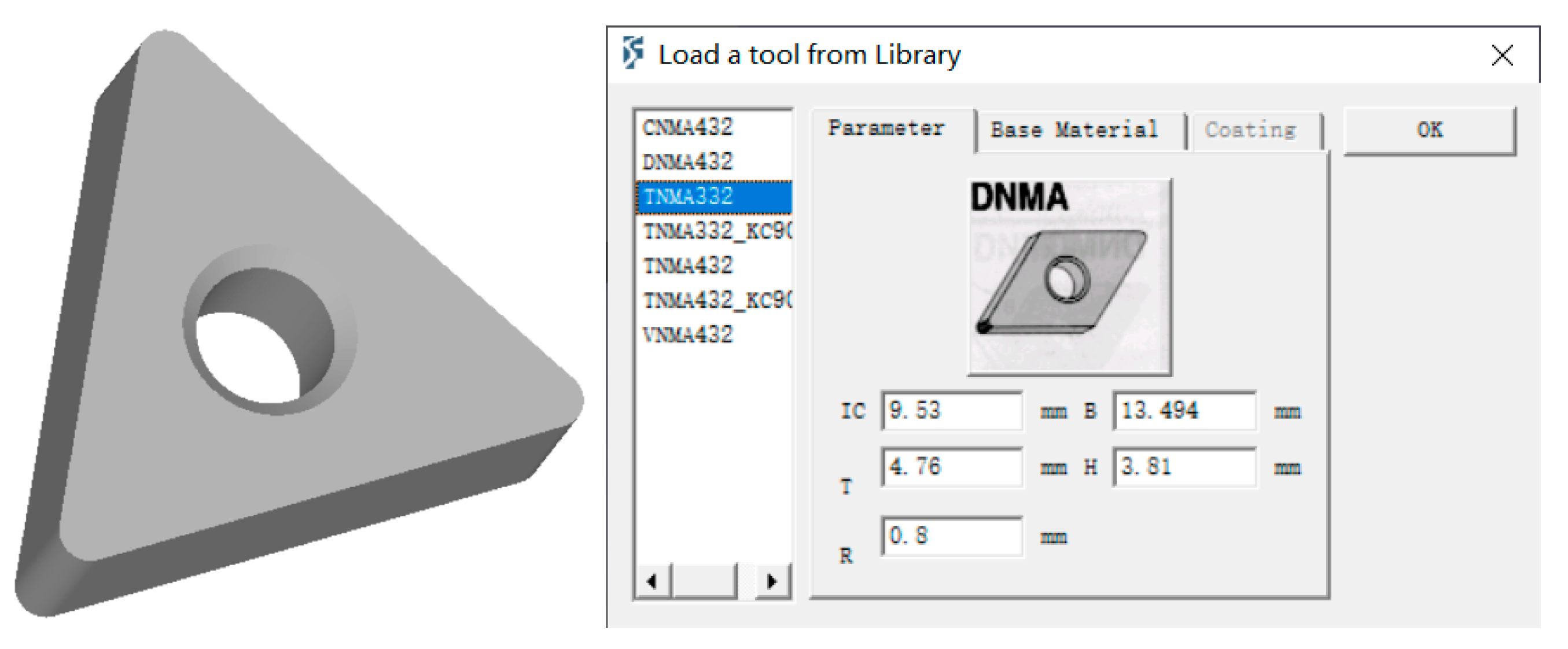
To further investigate the modeling capabilities of KAN-A/B/C on tool wear, we conducted additional simulation turning tests using DEFORM-3D software (version 11.0). Compared with ABAQUS and ANSYS (https://www.ansys.com/), DEFORM-3D offers distinct advantages, including a comprehensive material library, rational mesh generation, and efficient data acquisition. The turning simulation was performed using TNMA332 tools with key parameters configured, as shown in Figure 8.

AISI-1045 steel was selected as the workpiece material due to its excellent machinability, weldability, and broad applicability across mechanical manufacturing, automotive, and aerospace industries. Its physical and mechanical properties are presented in

Table 10. Physical properties of AISI-1045 steel.

Young’s Modulus (GPA)	Poisson’s Ratio	Density (kg/m2)	Thermal Expansion Coefficient (×10−6/°C)	Specific Heat Capacity (J/kg·°C)	Hardness (HB)
210	0.269	7860	12.6	500	200

.

The cutting parameters were set as follows: a cutting speed of 250 mm/s and a depth of cut of 0.5 mm along the lathe’s Y-axis. The Johnson–Cook constitutive model was employed to characterize the workpiece material’s dynamic behavior, while the normalized C&L fracture criterion served as the separation criterion. A shear friction model with a coefficient of 0.45 was applied to the tool–workpiece interface.

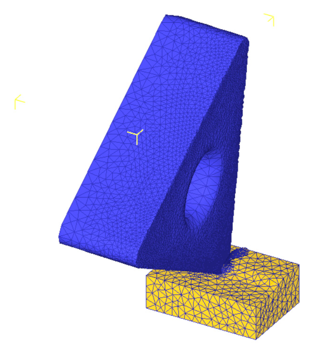
During simulation, DEFORM-3D performed dozens to hundreds of adaptive remeshing operations to accommodate severe material deformation. The computational efficiency was optimized by: (1) implementing local mesh refinement exclusively in the cutting zone, (2) adopting absolute meshing for the workpiece, with the minimum element size set at 40% of the feed rate, and (3) maintaining a ratio of 7.

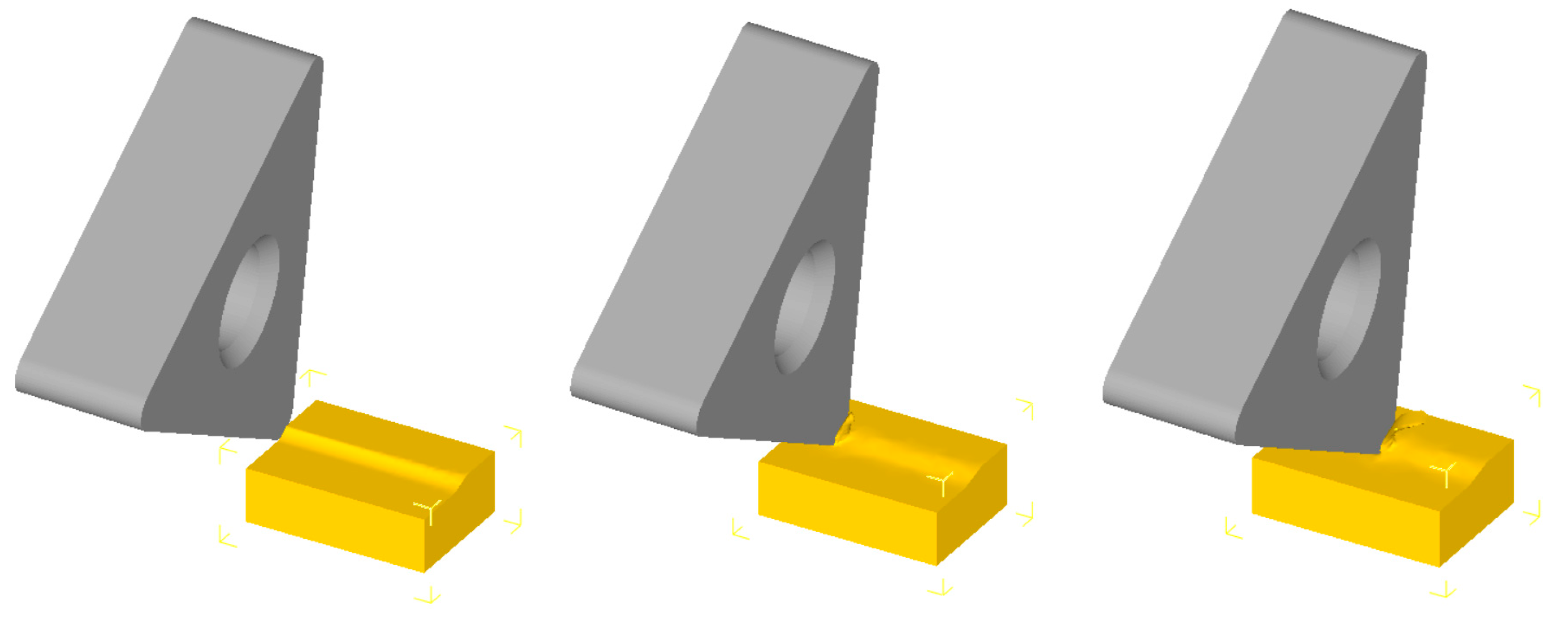
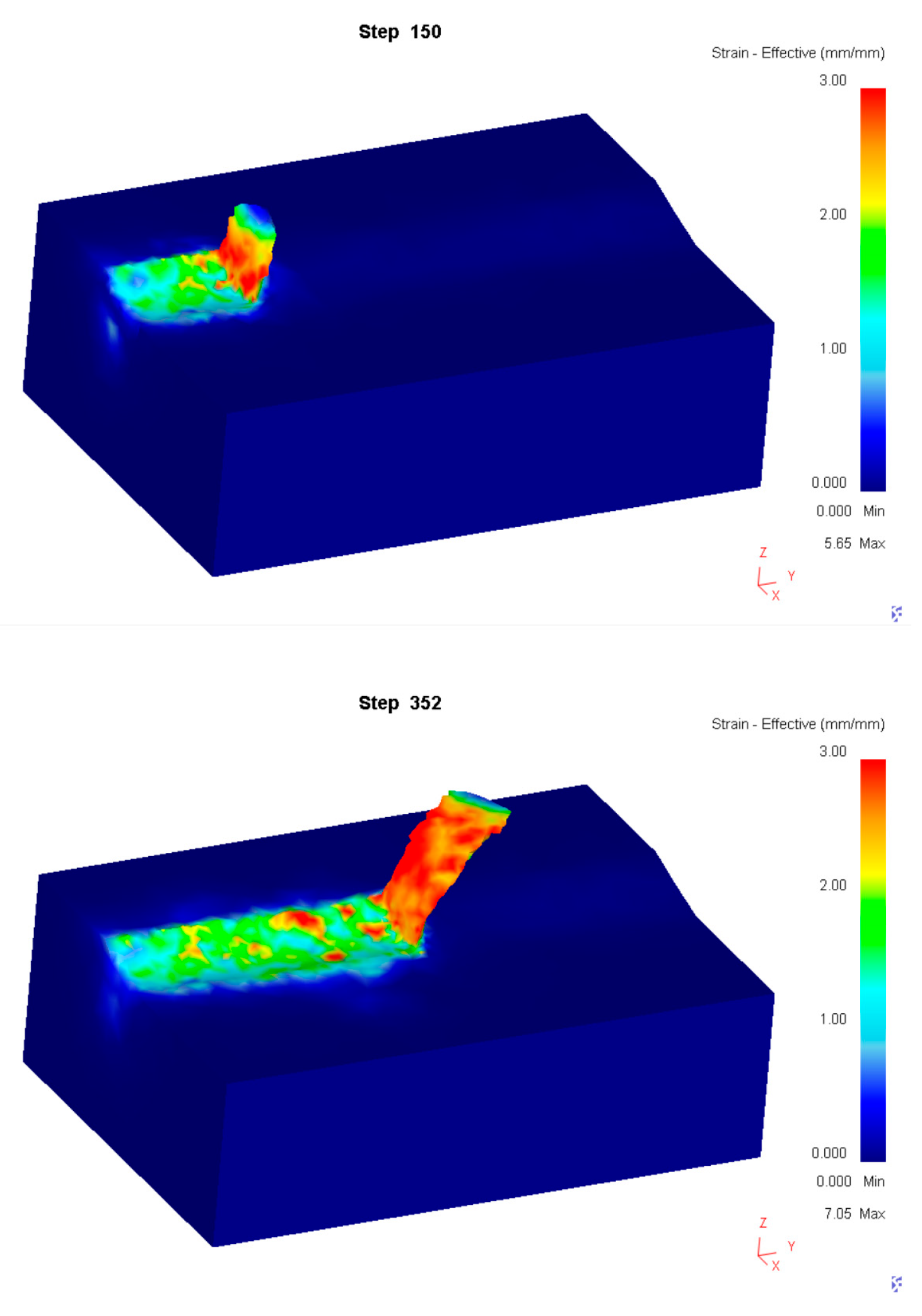
During the turning process, the relative positional relationship between the tool and workpiece is illustrated in Figure 9. The mesh deformation of the workpiece is shown in Figure 10. The temperature variation in the contact zone between the workpiece and cutting tool is presented in Figure 11.

After completing the simulated turning tests, the data on tool wear progression were obtained. Only the data samples corresponding to each observed change in tool wear were retained, as these points better represent the interaction characteristics between the tool and workpiece. For instance, during the stable wear phase, the wear amount of the cutting edge remains nearly constant, with minimal impact on part machining accuracy and surface quality.

This data processing approach helps verify whether the proposed method can effectively learn wear progression patterns. After processing, 350 samples were obtained and divided equally into training and test sets for model development.

The acquired data samples were further categorized into distinct features, with their definitions and explanations provided in

Table 11. Features and descriptions of simulated turning data samples.

Name	Definition and Description	Category
Step	Time step (the number of times processing time and parameters are recorded)	Feature
Time (s)	Cumulative machining time
Temperature (°C)	Temperature at the chip-tool contact area during turning
X/Y/Z-load (N)	Cutting forces acting on the tool in the X/Y/Z-axis directions
X/Y/Z-speed (mm/s)	Movement speed of the tool in the X/Y/Z directions
Wear depth (μm)	Tool wear depth	Modeling Target

.

7.2. Modeling Results of KAN-A/B/C and Discussion of Their Physical Significance

Subsequently, KAN-A/B/C were, respectively, employed to model and predict tool wear in simulated turning operations. All formulas retained four decimal places for precision. The formulas demonstrate the following:

$$\mathrm{KAN}\text{-}\mathrm{A}:0.0814{(-0.0019x_1-1)}^2-0.0775$$

(19)

$$\mathrm{KAN}\text{-}\mathrm{B}:0.0358{(0.0034x_1+1)}^2-0.0561+{\displaystyle \frac{0.1317}{7.2778-0.0087x_3}}$$

(20)

$$\mathrm{KAN}\text{-}\mathrm{C}:0.0004x_1-0.0021$$

(21)

where x₁ (step) was identified by all three KAN architectures as a significant variable influencing tool wear. KAN-B specifically indicated that increasing x₃ (temperature) accelerates tool wear progression.

It is readily apparent that KANs’ computational approach differs from conventional physics-based analysis. In other words, physics-driven formula derivation focuses on clarifying physical meanings and analyzing physical processes, providing researchers and engineers with broad reference values.

In contrast, KAN-based modeling primarily depends on the sample data itself. It can establish explicit ‘white-box’ formulas within given sample ranges. These formulas yield accurate modeling and prediction results, though they do not guarantee physical accuracy.

Thus, KANs can be characterized as a data-driven method that produces explicit formulas with potential physical interpretability. Compared to traditional “black-box” methods, KANs offer superior physical interpretability, though their derived formulas may not always align with physical assumptions.

Tool wear is a dynamic process involving multi-physics coupling (thermal, mechanical, and material deformation effects). In the current prediction results, KANs achieve explicit modeling through univariate or bivariate functions, specifically by establishing functional relationships between the time step (‘step’) and contact zone temperature (‘temperature’). The variable ‘step’ was identified by all KAN architectures as strongly correlated with the wear amount, consistent with the cumulative nature of tool wear. The role of ‘temperature’ reflects its direct influence on the hardness and chemical stability of tool materials under elevated temperatures.

However, KANs do not account for the influence of cutting forces and cutting speeds on tool wear, which are typically critical factors in physics-based modeling. It suggests that, as a data-driven regression method, KANs may struggle to incorporate the assumptions and constraints inherent in physical principles.

On the other hand, KANs’ characteristics offer new insights for advancing tool wear research. While many traditional models are highly accurate and meaningful, they often rely heavily on empirical formulas or physics-based derivations. Such physics-based models require extensive experimental calibration of parameters. Conversely, KANs adopt a data-driven approach to directly learn the implicit relationships among machining parameters, thereby reducing manual intervention.

Consequently, KAN-based regression and derivation are more outcome-oriented. The formulas provided by KAN-A/B/C achieve minimal errors and high R² values during both training and prediction phases, as demonstrated in

Table 12. KAN-A/B/C prediction errors of tool wear in simulated turning operations.

Model	Category	Error	Value
KAN-A	Train	MSE	3.11 × 10−6
		MAE	0.0014
		sMAPE	5.2634
		MaxAE	0.0045
		R2	0.9980
		Adjusted R2	0.9979
	Test	MSE	3.19 × 10−6
		MAE	0.0015
		sMAPE	6.8090
		MaxAE	0.0045
		R2	0.9983
		Adjusted R2	0.9982
	Runtime	Time	335.9916 s
KAN-B	Train	MSE	2.17 × 10−6
		MAE	0.0011
		sMAPE	3.9814
		MaxAE	0.0043
		R2	0.9987
		Adjusted R2	0.9986
	Test	MSE	2.34 × 10−6
		MAE	0.0012
		sMAPE	3.7332
		MaxAE	0.0043
		R2	0.9987
		Adjusted R2	0.9986
	Runtime	Time	288.3024 s
KAN-C	Train	MSE	1.01 × 10−5
		MAE	0.0028
		sMAPE	10.7109
		MaxAE	0.0065
		R2	0.9942
		Adjusted R2	0.9939
	Test	MSE	9.88 × 10−6
		MAE	0.0028
		sMAPE	12.3098
		MaxAE	0.0062
		R2	0.9941
		Adjusted R2	0.9938
	Runtime	Time	347.6650 s

.

Unlike conventional deep learning methods, which typically require large, labeled datasets, KANs achieve stable predictions in the experiment using only 350 samples (with a 1:1 training–test split).

Provided that machining conditions remain unchanged, the formulas derived by KANs hold significant reference value for tool wear prediction. Moreover, although the physical interpretability of KAN-A/B/C’s formulas is limited, they are explicit functions, enabling intuitive analysis of the relationship between input parameters and tool wear.

8. Conclusions

This study presented a progressively complex model system (KAN-A/B/C) based on KANs. Initially, tool wear modeling was conducted using flank wear data for turning tools obtained from Kaggle. Physically interpretable analytical expressions were proposed for tool wear prediction, establishing a foundation for real-time wear calculation under complex working conditions.

Subsequent vertical (intra-method) comparisons among KAN-A/B/C employed six error metrics and the computational time, revealing quantitative relationships between model complexity and prediction accuracy/efficiency. For horizontal comparison, isomorphic MLP benchmark models were developed, demonstrating KANs’ superiority in generalization performance and convergence stability across training, parameter, and basic principles. The comprehensive advantages of KANs in prediction accuracy and physical interpretation were further examined through comparisons with traditional empirical formulas (Usui Model) and machine learning methods.

Following this, turning simulations were implemented using DEFORM-3D, with the resultant data samples serving to validate the modeling capabilities of KAN-A/B/C. An in-depth discussion addresses the characteristics and limitations of the KAN-based “white-box” tool wear formula. KANs integrate data adaptability with mechanistic interpretability, and their reduced parameter count alongside high accuracy suggest that KANs offer a more efficient alternative. These findings underscore their uniqueness in manufacturing process modeling.

8.1. Current Limitations of KANs

The data-driven tool wear modeling based on KANs exhibits several limitations. First, while KANs can derive explicit mathematical formulas compared to black-box models, these derived results do not fully align with conventional physical principles.

Second, KAN-A/B/C primarily focuses on achieving low training and testing errors within the given dataset, with limited incorporation of physical understanding. For instance, in tests on public datasets, KANs identified cutting speed (Speed) as a non-critical parameter. It does not negate the role of cutting speed but rather reflects its relatively weak influence within the specific data range used.

Furthermore, the mathematical relationships derived from KAN-A/B/C are strictly valid only within the training data range. Due to the absence of physical constraints in the symbolic formulas, extrapolation beyond these bounds may lead to inaccurate predictions. Compared to traditional MLPs, the optimization of B-spline basis functions and edge-based activation learning increases the computational overhead in KANs.

8.2. Future Research Directions

(1) Integration of KANs with Physical Models

Construct hybrid models by combining KANs with explicit physical equations to enhance robustness. For tool wear processes, compute predictions using physical equations first, then employ KANs to compensate for discrepancies between the calculated results and the actual wear measurements. Develop a white-box model, integrating physical knowledge with KAN inference capabilities.

(2) KAN-Based Monitoring, Prediction, and Parameter Feedback

Leverage KANs’ lightweight architecture with significantly fewer parameters than traditional neural networks to develop embedded systems for real-time monitoring and predictive analysis of tool wear states. Dynamically feed predictive outputs back into CNC systems to optimize cutting parameter configurations.

(3) Multi-Material and Multi-Tool Wear Prediction

Investigate the accuracy and generalization capability of KANs in wear modeling across dissimilar materials (e.g., titanium alloys and composites) and tool geometries (e.g., coated tools and indexable inserts).