A High-Resolution Spectral Analysis Method Based on Fast Iterative Least Squares Constraints

Abstract

The prediction of reservoir and caprock thickness is important in geological evaluations for site selection for aquifer underground gas storage. Therefore, high-resolution seismic identification of reservoirs and caprocks is crucial. High-resolution time–frequency decomposition is one of the key methods for identifying sedimentary layers. Based on this, we propose a least squares constrained spectral analysis method using a greedy fast shrinkage algorithm. This method replaces the traditional Tikhonov regularization objective function with an L1-norm regularized objective function and employs a greedy fast shrinkage algorithm. By utilizing shorter window lengths to segment the data into more precise series, the method significantly improves the computational efficiency of spectral analysis while also enhancing its accuracy to a certain extent. Numerical models demonstrate that compared to the time–frequency spectra obtained using traditional methods such as wavelet transform, short-time Fourier transform, and generalized S-transform, the proposed method can achieve high-resolution extraction of the dominant frequencies of seismic waves, with superior noise resistance. Furthermore, its application in a research area in southern China shows that the method can effectively predict thicker sedimentary layers in low-frequency ranges and accurately identify thinner sedimentary layers in high-frequency ranges.

1. Introduction

In site selection for aquifer underground gas storage, assessing geological conditions via trap evaluation is a key factor. In particular, the evaluation of the sedimentary thickness of the reservoir and caprock is directly related to the gas storage capacity and sealing performance of the aquifer trap [1]. The geological conditions in southern China are complex, and time–frequency analysis has become an important technology in research on strata sedimentary characteristics. A high-precision time–frequency decomposition method based on seismic identification is critical to the reliability of sedimentary layer thickness prediction.

Since Taner et al. (1979) utilized complex seismic trace analysis techniques for seismic signal analysis [2], the possibility that low-frequency anomalies are related to oil and gas reservoirs has become a widely acknowledged notion. Subsequently, several scholars have proposed various methods to extract frequency-related attributes for the interpretation of seismic data. Among these, the spectral decomposition method introduced by Partyka et al. (1999) has garnered widespread attention in reservoir characterization [3]. By utilizing seismic data and the Discrete Fourier Transform (DFT), the spectral decomposition method can reveal more stratigraphic details, allowing for the analysis of small-scale structures and seismic attenuation anomaly zones that are often closely associated with oil and gas reservoirs [4].

Time–frequency analysis is a technique that transforms seismic data from the time domain to the frequency domain through certain mathematical transformations. It decomposes seismic records into different frequency components and uses the varying response characteristics of different frequencies on geological bodies at various scales to interpret these geological bodies, thereby conducting seismic interpretation (a frequency-based reservoir interpretation technology) [5]. This technique allows for the analysis of amplitude corresponding to each frequency in the frequency domain, eliminating mutual interference between different frequency components in the time domain. Not only does it enhance the predictive capability of seismic data for thin reservoirs, but it also extracts richer geological information from conventional seismic datasets, improving the ability to interpret and identify special geological bodies.

Liu et al. explored small-scale geological issues of carbonate reservoirs using spectral decomposition through the establishment of a positive modeling model [6]. Liu et al. P proposed exploring corresponding time–frequency patterns for different geological conditions [7]; Zhu et al. introduced a spectral imaging method based on physical wavelet transform to finely characterize high-frequency energy [8]. Chang et al. [9] predicted the gas content of coal seams in a specified study area by utilizing spectral decomposition based on the high-frequency absorption and attenuation characteristics caused by coalbed methane (methane) enrichment. These studies demonstrate that spectral techniques have advantages over traditional seismic attribute methods in identifying structural fracture systems and predicting thin-layer thicknesses, and actively promote the application of spectral decomposition technology in coalfield seismic data analysis.

Spectrum decomposition is an earthquake attribute technology based on time–frequency analysis [10,11,12]. It processes seismic data into frequency slices, enabling thin-layer reflection systems to produce complex resonant reflections. Fundamentally, spectrum decomposition algorithms are methods for processing seismic reflection data by breaking down seismic information into frequency information. By selecting specific frequencies, it helps interpretation personnel effectively identify and extract hidden geological layers and structural features by browsing selected frequency data, fully tapping into the implicit geological information. Traditional seismic processing and interpretation techniques are influenced by seismic resolution; for faults smaller than 5 m, the verification rate is low. Using spectrum decomposition technology can effectively overcome the limitations of seismic resolution [13,14,15], better highlighting geological anomalies. At the same time, spectrum decomposition technology aids in displaying rock layer morphology, significantly enhancing the recognition of complex geological bodies [16].

Various algorithms are commonly employed to achieve spectral decomposition. Short-time Fourier transform (STFT) could be one of the most computationally cost-effective methods for spectral decomposition; however, a key challenge lies in selecting an appropriate window length that maintains both time and frequency resolution in the output. Another widely used spectral decomposition method is Continuous Wavelet Transform (CWT). The CWT method decomposes seismic traces into different frequency components using child wavelets with varying scales, effectively performing bandpass filtering in the time domain [17,18]. Compared to STFT, the CWT method is less affected by the choice of time window, as the spectral dictionary inherently incorporates frequency-related windows. It is important to note that the wavelets used in CWT must be orthogonal, and its output can also be obtained using STFT with an appropriate window function. Another class of spectral decomposition methods involves user-defined wavelet dictionaries. These methods typically yield results with high temporal and spectral resolution, but they come with significant computational costs. Due to their high-resolution advantages, many researchers are focused on improving their efficiency. Additionally, there are various other methods for decomposing seismic data into the time–frequency domain, each with its own advantages and potential effectiveness in specific situations [19].

STFT offers fixed time–frequency localization, but wavelet transform provides more flexible localization. For different frequency ranges, wavelets adjust the window size, which gives better time localization for high frequencies but poorer frequency resolution for low frequencies. While wavelet transform offers better time localization for non-stationary signals, particularly at high frequencies, it sacrifices frequency resolution, especially at low frequencies. This is why wavelet transform’s time–frequency resolution is often lower than that of STFT, especially in the low-frequency range. In summary, wavelet transform has more adaptive time–frequency localization but at the cost of frequency resolution, especially at lower frequencies, making its overall resolution sometimes lower than that of fixed-resolution STFT. In comparison, STFT provides a fixed frequency resolution for a given window size. This results in a more balanced time–frequency resolution across the entire spectrum. However, the fixed window in STFT does not adapt like wavelet transform, meaning the time–frequency trade-off is more uniform.

Currently, signal processing methods based on inversion concepts can enhance resolution or signal-to-noise ratio through iterative processes [20,21,22,23,24,25,26]. Similarly, inversion-based spectral decomposition methods are among the most effective techniques. The constrained least squares spectral analysis (CLSSA) proposed by [27] is a highly specialized spectral decomposition method that can handle both narrowband and broadband seismic data. The CLSSA method significantly reduces distortion caused by the window function effect by directly optimizing the L2-regularized least squares fitting function to solve for the Fourier coefficients. Ref. [27] demonstrated that the CLSSA method can accurately predict the Fourier spectrum even with very short window lengths [27]. Liu et al. (2014) applied Puryear’s inversion method to braided river and reservoir characterization, achieving favorable results [28]. Additionally, Zeng (2018) studied an iterative inversion spectral decomposition method based on shape regularization and applied it to the spectral analysis of gas-containing reservoirs [29]. Furthermore, shape regularization methods have shown promising results in one-dimensional data interpolation, velocity estimation, and local seismic attribute estimation.

Although the constrained least squares spectral analysis (CLSSA) method based on inversion concepts offers the advantage of high resolution, it has the drawback of being computationally expensive when dealing with large datasets. In numerical analysis and inversion, the L1 norm encourages sparsity, meaning it tends to produce solutions with many zero-valued coefficients, which is beneficial in feature selection and sparse modeling, particularly with high-dimensional data. Additionally, it is robust to outliers, as it minimizes the sum of absolute differences, making it less sensitive to extreme values. However, the L2 norm is sensitive to outliers, as squaring large errors disproportionately amplifies their influence, potentially skewing the model. Additionally, it does not encourage sparsity, yielding dense solutions that can increase model complexity, particularly in high-dimensional data. Therefore, this paper replaces the Tikhonov regularization objective function with the L1-norm regularization objective function in the CLSSA method, and employs a fast iterative algorithm to significantly enhance its computational efficiency. The structure of this paper is as follows: First, a brief introduction to the CLSSA method and its theoretical foundation is presented. Next, an improved iterative updating algorithm is introduced. Finally, the method is applied to a research area in southern China, demonstrating its effectiveness in practical applications and yielding high-resolution, reliable time–frequency spectrum profiles.

2. Theory

2.1. Principles of Least Squares Constrained Spectral Analysis

Seismic data can generally be represented using a convolution model as a superposition of wavelets with different amplitudes, dominant frequencies, and time shifts. Therefore, the seismic trace d can also be expressed as follows:

$$Fm=d$$

(1)

where m represents the frequency spectrum of the seismic signal, which is equivalent to the Fourier transform coefficients. The matrix F is a kernel matrix composed of sine signals within the truncated frequency and time range. Its row vectors represent the range of frequency values, while its column vectors indicate the relative time of the window function. This can be expressed as follows:

$$F\left(t,f\right)=\cos \left(2\pi ft\right)+i\sin \left(2\pi ft\right)$$

(2)

From Equation (2), it can be seen that Equation (1) can be considered the matrix representation of the discrete Fourier transform. Ref. [27] proposed the CLSSA method based on Equations (1) and (2) [27]. This method can be formulated as a least squares problem, expressed as follows:

$$\min \left({‖F_w{m}_w-W_{d}d‖}^2+\lambda {‖m_w‖}^2\right)$$

(3)

The constrained kernel matrix F_w = W_dFW_m represents the complex sinusoidal signals of the model W_m and the data weights W_d, and the symbol * stands for the matrix transpose operator. The vector m_w= W_m⁻¹m is the modified model parameter vector (which requires the introduction of model weights to calculate the frequency coefficients), where W_d denotes the data weights. In Equation (3), $\lambda {‖m_w‖}^2$ is the regularization term, which is introduced to address the problem of solving ill-posed matrices. $\lambda$ is the regularization parameter, which can be adjusted to control the sparsity and stability of the solution. As $\lambda$ increases, the model’s variance decreases, but the bias of the estimates from the true values increases, leading to a greater model bias. Therefore, it is essential to choose a reasonable $\lambda$ to balance the model’s variance and bias. When selecting $\lambda$, one should ensure that the method is robust to noise in the data. Typically, it is set to 0.001 times the maximum value on the diagonal of the weighted Gram matrix. Generally, models are constructed with small parameters, allowing them to easily adapt to different datasets. This way, even if the data have slight deviations, they will not significantly impact the results, and it can help mitigate overfitting to a certain extent.

By solving Equation (3), the frequency spectrum of the seismic signal can be obtained as follows:

$$m_w=F_w^{*}{\left(F_w{F}_w^{*}+\lambda I\right)}^{-1}{W}_{d}d$$

(4)

The matrix inversion in this equation is computed using the Gaussian elimination method. Iteration is achieved by updating the model weights of the frequency spectrum at the center of the window. Increasing the number of iterations will make the solution sparser and yield a more compact frequency spectrum.

2.2. Objective Function

Compared to L2 regularization, L1 regularization can also help prevent overfitting to a certain extent. The L1 norm promotes a sparse model by reducing some unimportant regression coefficients to zero. This reduction in computation can lead to lower average errors, thereby decreasing model complexity and potentially improving fitting performance. Therefore, to enhance the convergence speed of the spectral analysis method, we can replace the L2 norm in objective functional 3 with the L1 norm. The modified equation can be expressed as follows:

$$\underset{x}{\min }{\displaystyle \frac{1}{2}}\Vert F_w{m}_w-W_{d}d{\Vert }^2+\lambda \Vert m_w{\Vert }_1$$

(5)

However, since the regularization term in Equation (5) is the L1 norm, it is non-differentiable, which prevents the use of gradient descent for optimization. Therefore, this paper employs the Iterative Shrinkage–Thresholding Algorithm (ISTA) to address this issue, utilizing a proximal gradient descent approach.

2.3. Fast Iterative Shrinkage–Thresholding Algorithm

Among the numerous gradient-based algorithms, the Iterative Shrinkage–Thresholding Algorithm (ISTA) is a highly regarded method. The ISTA updates the least squares solution in each iteration through a shrinkage/soft-thresholding operation, and its specific iterative format is expressed as follows:

$$m_{k+1}=sof{t}_{\lambda t}\left(m_k-2t{F_w}^T\left(F_w{m}_k-W_{d}d\right)\right)$$

(6)

The threshold operation function is

$$sof{t}_T\left(m_i\right)=\mathrm{sgn}\left(m_i\right)\left(\left|m_i\right|-T\right).$$

(7)

In Equation (6), t represents the iteration step. As can be seen from Equation (6), during each iteration process, the ISTA only considers the information at the current point to update the iteration starting point, which results in a relatively slow convergence speed for the algorithm. The Fast Iterative Shrinkage–Thresholding Algorithm (FISTA) builds upon the ISTA by considering both the current point and the previous point to update the iteration starting point, thereby achieving a faster convergence speed compared to the ISTA. The flow of the FISTA is as follows:

• Input time–space domain seismic data d and the maximum number of iterations K;
• Initialize the model m₀, current iteration count k = 0, and step t > 0, p₀ = 1, y = m₀;
• If $k\le K$, perform iterative updates;
• Output the frequency spectrum of the seismic data mk.

Compared to the ISTA, the FISTA uses y_k instead of m_k. In the iterative process, the iteration point mk of the FISTA not only depends on the previous iteration point m_k−1 but also utilizes a linear combination of the two previous points $\left\{m_{k-1},m_{k-2}\right\}$, thereby improving convergence speed. The inertia parameter a_k controls the growth rate of $m_k-m_{k-1}$.

The ISTA is straightforward to compute but converges slowly. Although the FISTA converges faster than the ISTA, it can exhibit oscillations when $a_k\to 1$, which slows down convergence. Handling massive seismic datasets imposes higher efficiency requirements on algorithms. The Greedy Fast Shrinkage Algorithm (GFISTA) [30] maintains computational simplicity while achieving faster global convergence rates than the ISTA and FISTA, with improved convergence performance [30]. This paper applies the GFISTA to spectral analysis algorithms, proposing a least squares constrained spectral analysis method based on fast iterative shrinkage. The GFISTA proceeds as follows:

• Input time–space domain seismic data d and the maximum number of iterations K;
• Initialize the model m₀, current iteration count k = 0, and iteration step t > 0, y₁ = m₀, the shrinkage factor of the step $\xi <1$, and the control factor for algorithm convergence $S>1$;
• If $k\le K$, perform iterative updates:

  $$\begin{array}{c}{y}_k=\left(m_k-m_{k-1}\right)\\ m_{k+1}=sof{t}_{\lambda t}\left\{y_k+2t{F}^{-1}\left\{{\left(F^{H}F\right)}^{-1}\times F^H\left(F_w\left(y_k\right)-W_{d}d\right)\right\}\right\}\\ k+1\to k\end{array}$$

  (8)

• Restart condition: if ${\left(y_k-m_{k+1}\right)}^T\left(m_{k+1}-m_k\right)\ge 0$, $y_k=m_k;$
• Convergence condition: if $‖m_{k+1}-m_k‖\ge S‖m_1-m_0‖$, $t=\max \left\{\xi t,t\right\}$ $k+1\to k$.

4.

Output the frequency spectrum of the seismic data mk. In this algorithm, $t\in \left[1/{\lambda }_{\max }\left(F^{H}F\right),2/{\lambda }_{\max }\left(F^{H}F\right)\right]$.

To address the oscillation issue caused by $a_k\to 1$ in the FISTA, the Greedy FISTA introduces a restart mechanism where $a_k\to 1$ periodically. This forces a_k to start increasing from 0 again, effectively preventing oscillations that occur when $a_k\to 1$ and restarting the process in a cycle. To minimize the interval between restarts and reduce the oscillation period, thereby improving the convergence rate, a_k is set to a constant value of 1. This restart framework ensures convergence while shortening the restart interval and oscillation period. Compared to the ISTA and FISTA, this approach enhances convergence speed.

3. Model Test

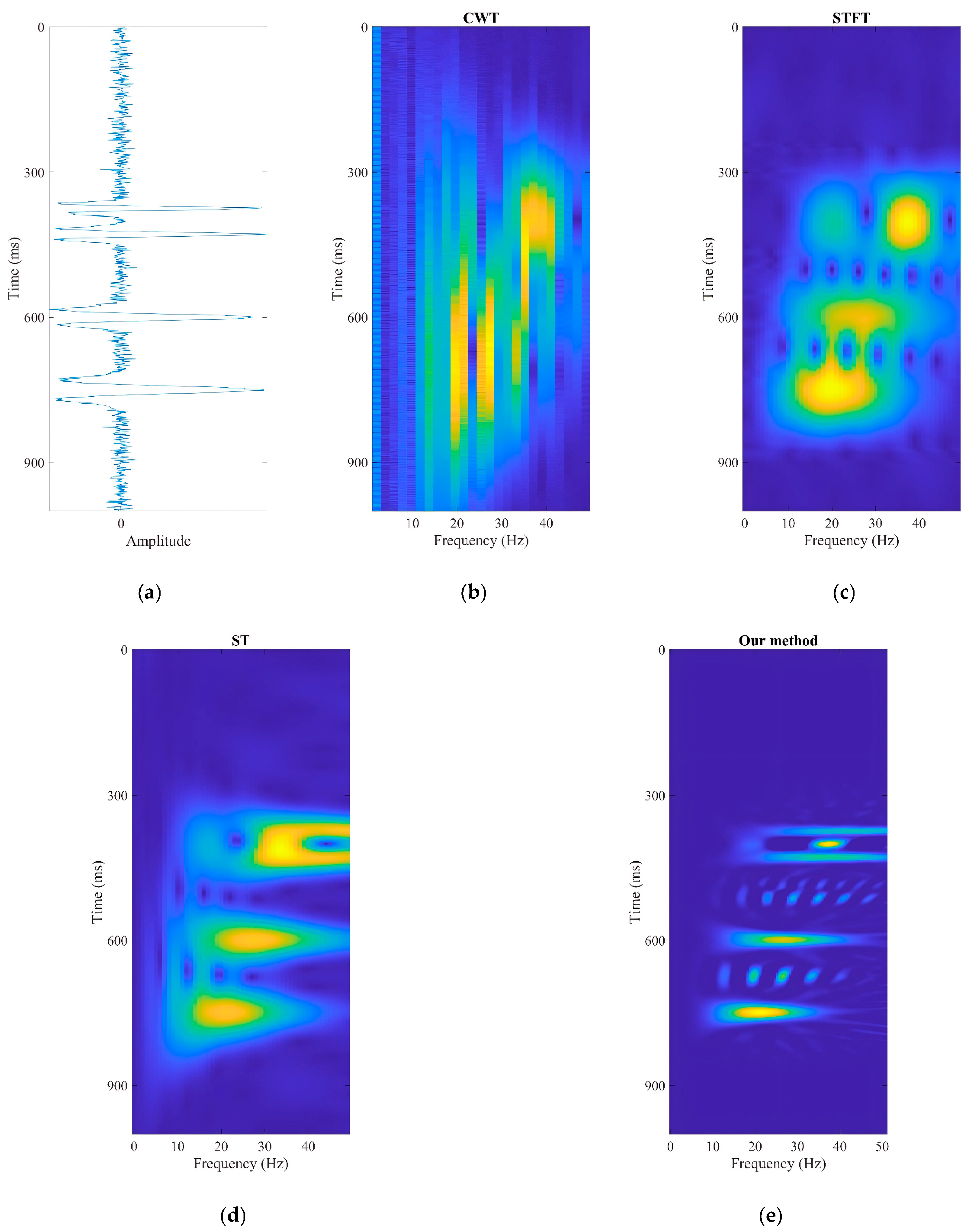
To demonstrate the effectiveness of the proposed method, Figure 1a shows a single seismic trace with a signal-to-noise ratio (SNR) of 20 dB, containing four seismic wavelets with central frequencies of 15 Hz, 20 Hz, 25 Hz, and 30 Hz. Figure 1b–d display the time–frequency spectra obtained using wavelet transform, short-time Fourier transform, and generalized S-transform, respectively. And the window length for all the compared methods is all 40 ms. As seen from the figures, the time–frequency resolution obtained by wavelet transform is the lowest, making it difficult to effectively distinguish the frequency-domain characteristics of the seismic waves. Compared to wavelet transform, both short-time Fourier transform and generalized S-transform are able to capture the seismic wave characteristics, but with very low resolution, failing to accurately extract the dominant frequency information of the seismic waves. In contrast, as shown in Figure 1e, the time–frequency spectrum obtained using our method can extract the dominant frequencies of seismic waves with high resolution, which is of significant importance for identifying gas-bearing formations.

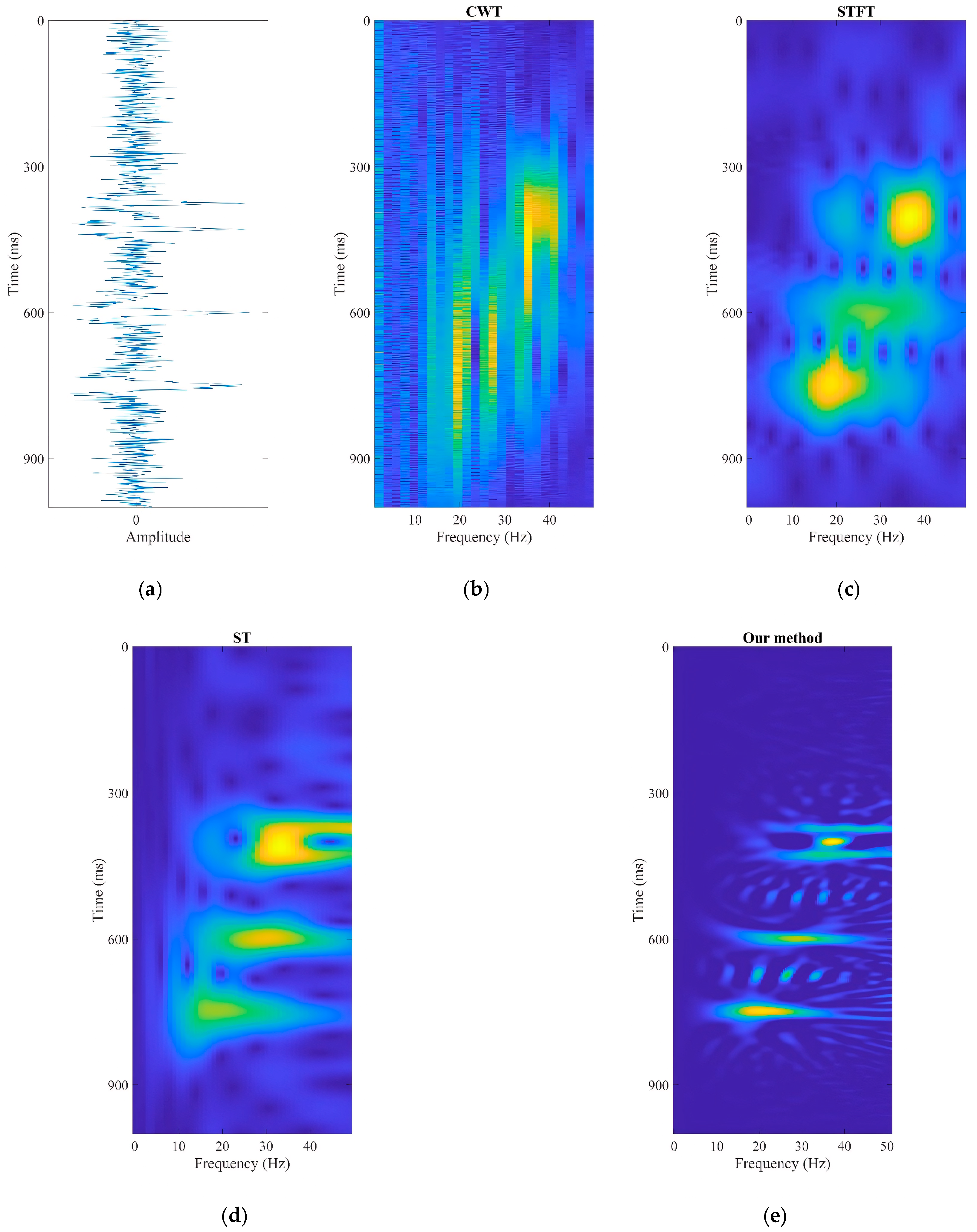
To further illustrate the noise robustness of the proposed method, we reduced the SNR of the single seismic trace shown in Figure 1a to 10 dB and extracted the corresponding time–frequency spectra using the same methods. A comparison between Figure 1e and Figure 2e shows that, even under extremely low SNR conditions, our method is still able to accurately extract the time–frequency characteristics of the seismic waves, while other methods are greatly affected by noise, significantly compromising the accuracy of the time–frequency spectra.

Given the typically large volume of seismic data, computational efficiency is a critical factor in practical applications. As shown in

Table 1. Elapsed time for different time–frequency spectra.

Method	CWT	STFT	ST	Our Method
Elapsed time (s)	0.086	0.077	0.175	0.0021
Speed-up ratio	40.9	36.6	83.3	1.0

, we have evaluated and compared the computational efficiency of our method with other time–frequency analysis techniques. The results in Table 1 demonstrate that our proposed method outperforms the others in terms of efficiency, ensuring its practicality for real-world use.

4. Field Data Example

The main area of operation is located in southern China. The sedimentary characteristics in the study area are complex. To better identify sedimentary layers, this study applies time–frequency analysis to seismic data, using different objective functions to assist in mapping stratigraphic features. Four spectral decomposition methods—STFT, CWT, CLSSA, and CLSSA based on the Greedy FISTA—are applied to actual seismic data to analyze their time–frequency spectrum characteristics. This study compares their computational efficiency, effectiveness, and stability.

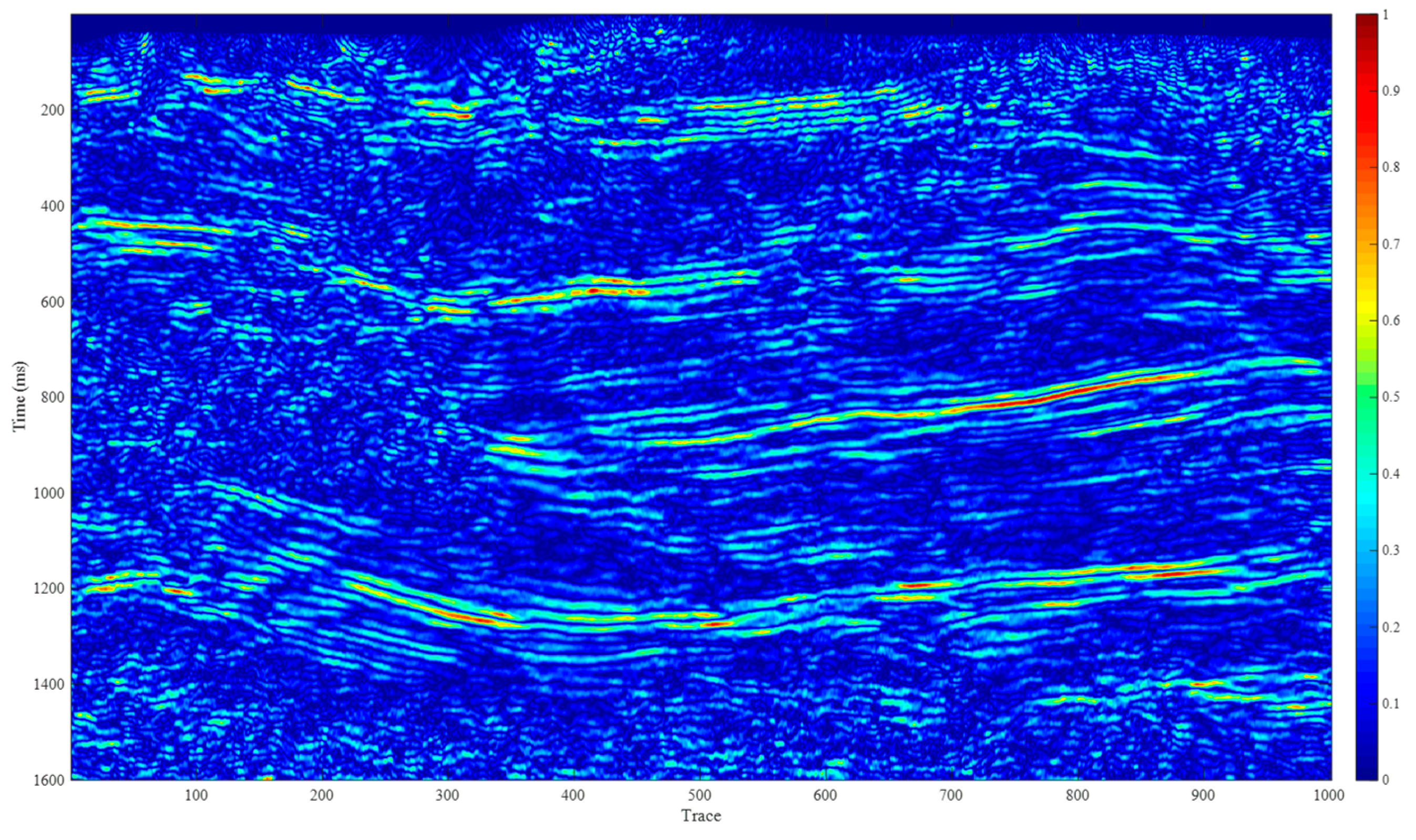
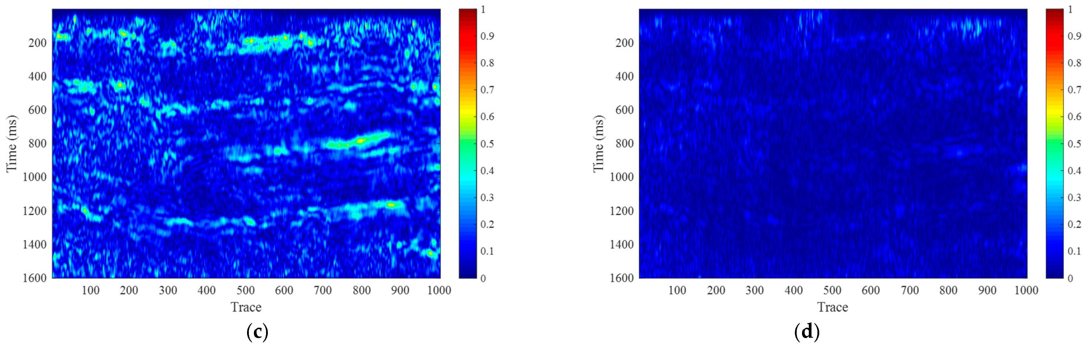
Figure 3 shows the actual seismic section profile. Figure 4 presents the time–frequency analysis frequency attribute maps using the STFT method. Specifically, Figure 4a shows the 10 Hz profile, Figure 4b displays the 20 Hz profile, and Figure 4c,d depict the 40 Hz and 60 Hz time–frequency spectrum profiles, respectively. In STFT, spectral distortion is more pronounced within short windows. In this study, a 40 ms time window is used for time–frequency analysis to ensure sufficient time resolution at low frequencies. As shown in Figure 4, the STFT method exhibits good lateral continuity of the time–frequency spectrum. However, due to the spectral tailing effect, the frequency energy in the STFT method appears blurry and shifts toward higher frequencies across all characteristic frequency attribute maps. This causes the frequency details to be less clearly highlighted.

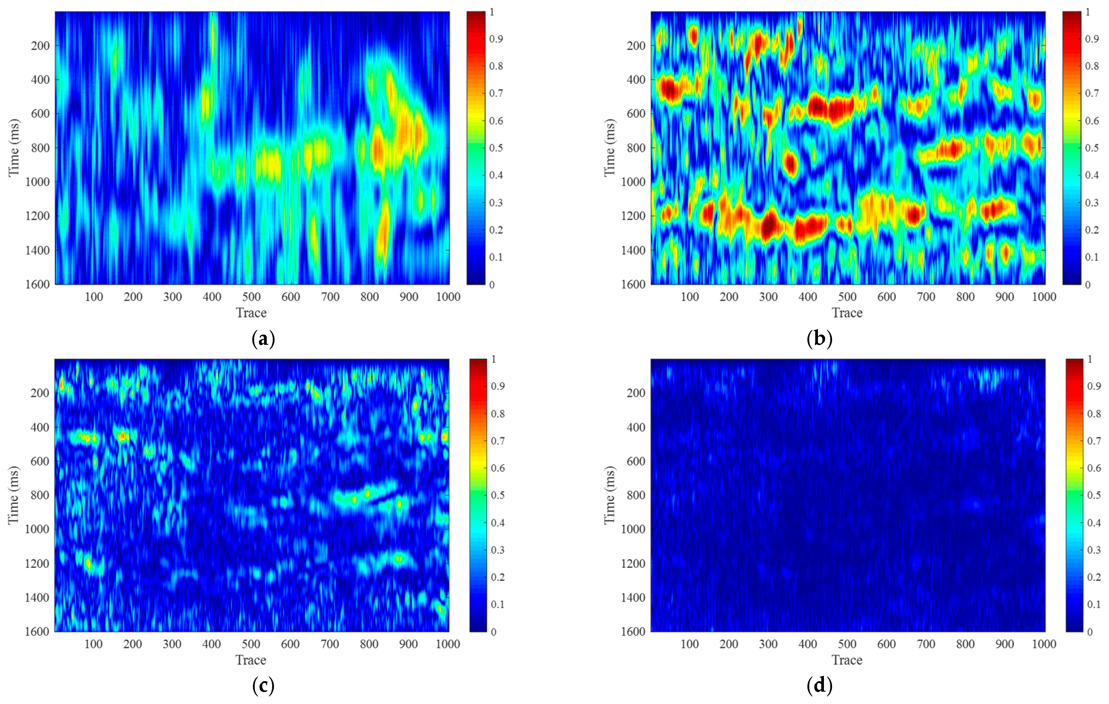
Figure 5 shows the time–frequency analysis frequency attribute maps using the CWT method. Specifically, Figure 5a presents the 10 Hz profile, Figure 5b shows the 20 Hz profile, Figure 5c displays the 40 Hz profile, and Figure 5d shows the 60 Hz profile. By comparing Figure 4a,b and Figure 5a,b, it is evident that the CWT method exhibits very low time resolution at low frequencies, failing to effectively display spectral characteristics at high resolution. The primary reason for this is that the CWT method does not use a time window to isolate seismic events, which prevents local analysis, resulting in very low time resolution at low frequencies.

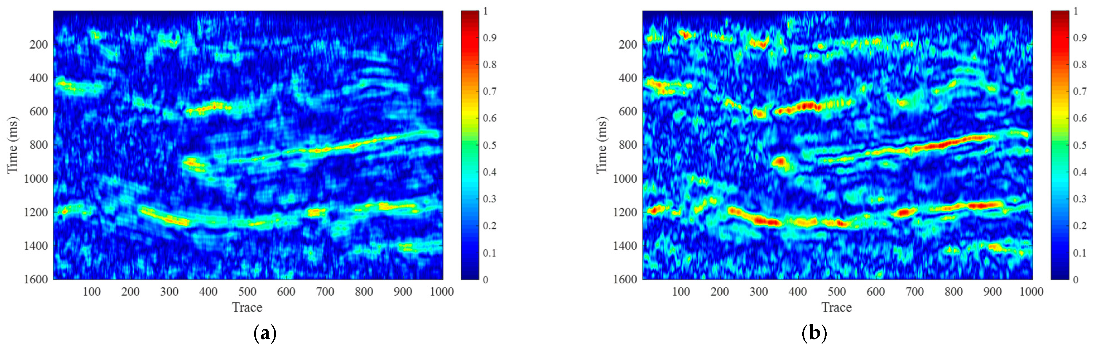
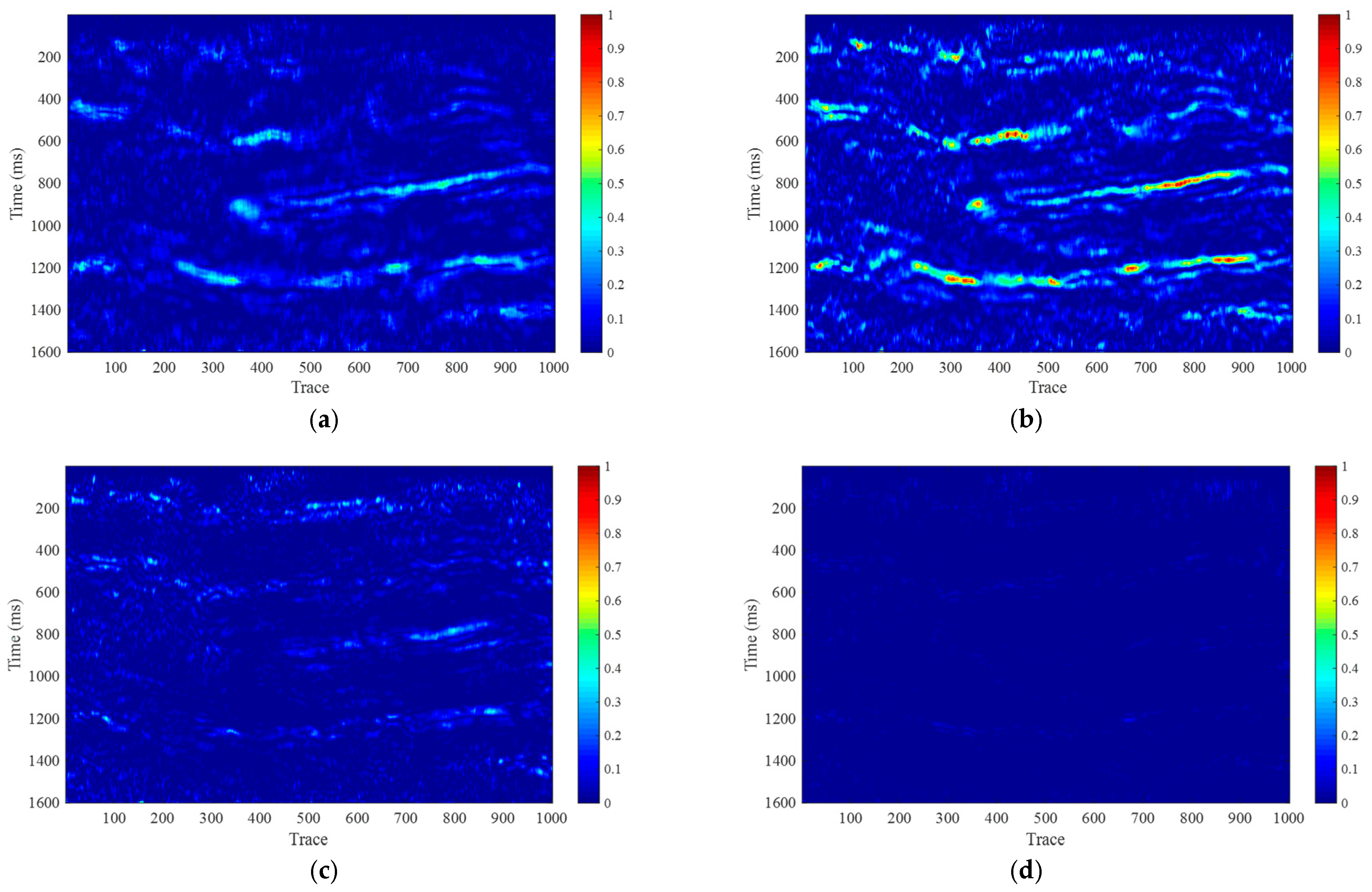
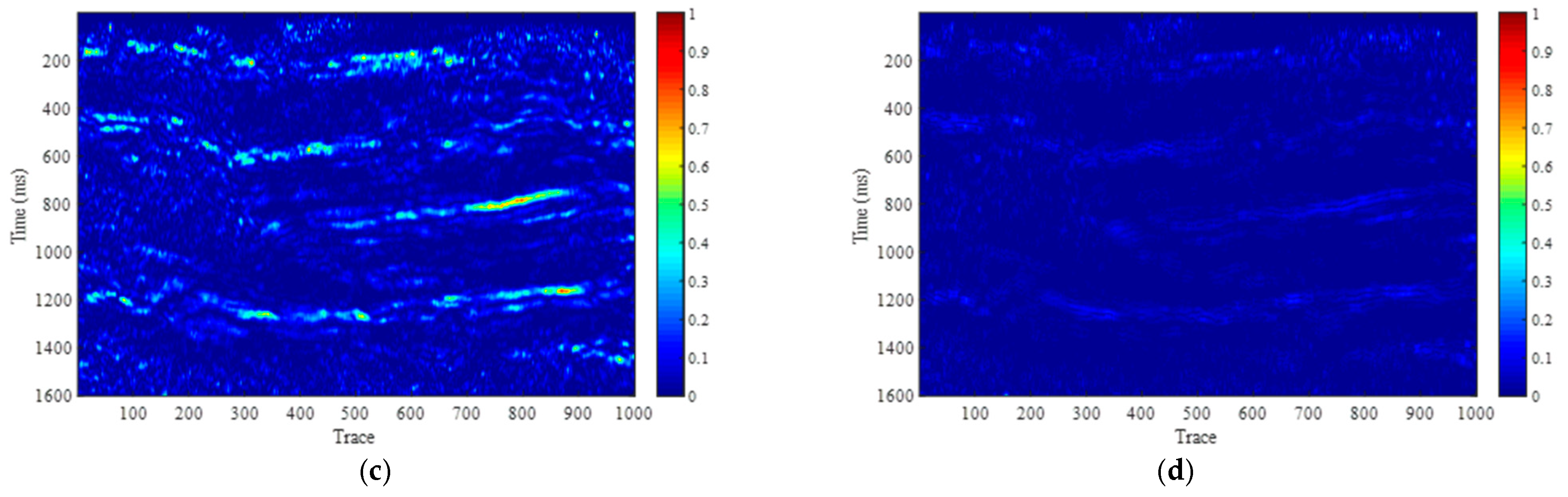
Figure 6 illustrates the time–frequency analysis frequency attribute maps using the CLSSA method. Similar to the STFT and CWT methods, Figure 6a,b represent the 10 Hz and 20 Hz time–frequency spectrum profiles, while Figure 6c,d correspond to the 40 Hz and 60 Hz profiles. A 30 ms time window is used for time–frequency analysis. Through comparison with Figure 4, it can be seen that the least squares constrained spectral analysis method can achieve high-resolution spectral analysis at both low and high frequencies, with higher resolution than the STFT method. 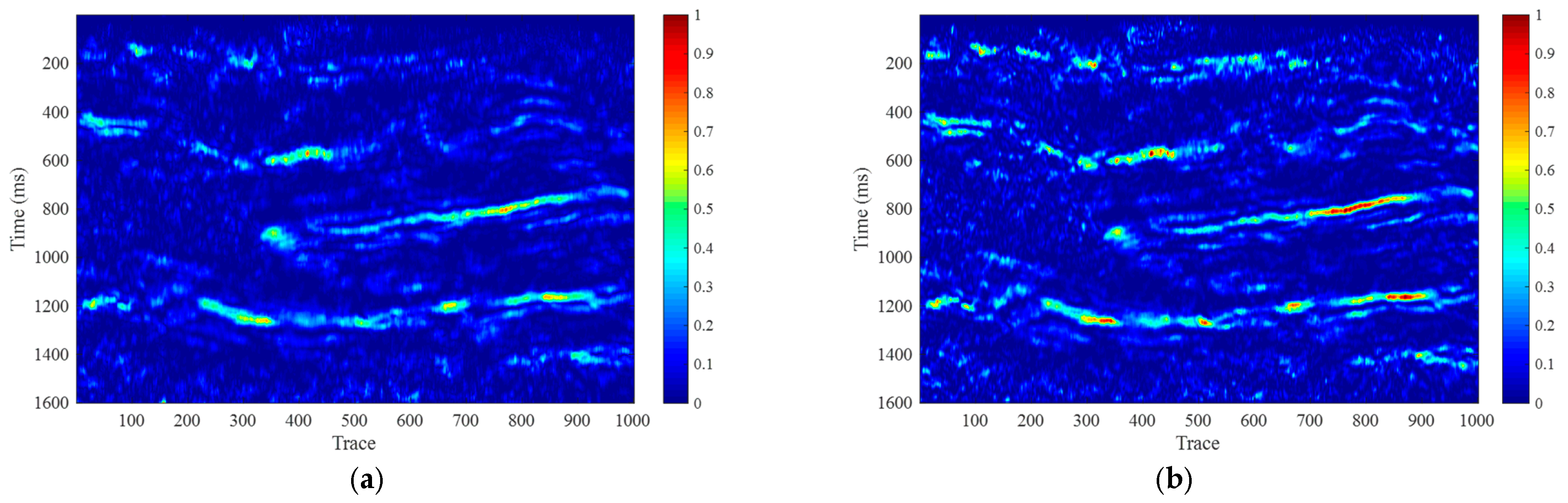Figure 7 shows the time–frequency analysis frequency attribute maps using the CLSSA method based on the Greedy FISTA. Figure 7a–d correspond to the 10 Hz, 20 Hz, 40 Hz, and 60 Hz profiles, respectively. By comparing this method with the traditional CLSSA method, it is evident that the proposed method achieves higher time–frequency resolution at both high and low frequencies, with a resolution significantly better than that of the STFT and CWT methods.

From the above comparative analysis, it is clear that both the CLSSA method and the Greedy FISTA-based CLSSA method offer high stratigraphic resolution in frequency attribute maps, effectively highlighting the characteristics of the target layers. These methods mitigate the window tailing effect of STFT and the low time resolution of CWT at low frequencies. The CLSSA methods accurately emphasize thicker sedimentary layers at 10 Hz and thinner layers at 40 Hz, providing more precise estimates of layer thickness.

In terms of computational efficiency, all four spectral decomposition methods were executed using a 6-CPU parallel pool (intel i7-12700). From Table 1, the computation times for the four methods are as follows: 80.2696 s for the STFT method, 75.8616 s for the CWT method, 275.6139 s for the CLSSA method (with two iterations), and 156.2003 s for the Greedy FISTA-based CLSSA method. Although the STFT and CWT methods offer higher computational efficiency, their spectral resolution is lower, especially at low frequencies where they fail to effectively display meaningful spectral characteristics. Compared to the traditional least squares constrained spectral analysis method, the Greedy FISTA-based CLSSA method significantly improves computational efficiency and enhances spectral resolution across different frequencies. This method provides a more accurate description of sedimentary layers, offering critical insights into predicting reservoir and caprock thickness.

5. Discussion

Time–frequency analysis can highlight the detailed characteristics of stratigraphy, while frequency attribute analysis can reveal subtle structural features in broadband amplitude maps. Ideally, time–frequency analysis aims to achieve high temporal resolution while also obtaining high frequency resolution through the use of short windows.

In traditional spectral analysis methods, CWT struggles to perform local analysis because it does not use time windows to isolate seismic events, resulting in very low time resolution at low frequencies. The results from STFT are difficult to distinguish in detail due to the effects of frequency decay and severe window tailing. However, the least squares constrained spectral analysis method significantly reduces spectral leakage by solving the non-zero diagonal term information. With short windows, it can emphasize various frequency features, highlighting thicker layers in low-frequency profiles and thinner layers in high-frequency profiles. By incorporating prior information constraints, it weakens the spectral smoothness of windowed data, allowing short windows to achieve a high time resolution and more accurately invert the amplitude spectrum of seismic reflection waves.

The Greedy FISTA spectral analysis method used in this study accelerates convergence speed through large-step iterations. To prevent divergence, a strictly less-than-1 parameter shrinkage step size is employed, ensuring that each iteration uses a locally optimal step size strategy to improve inversion efficiency. Additionally, the Greedy FISTA can eliminate high-frequency artifacts caused by noise in the CLSSA method, providing greater robustness and accuracy in resolution.

The numerical model and its application to field data prove that our proposed method can achieve a higher resolution than traditional methods, such as wavelet transform, short-time Fourier transform, and generalized S-transform. This will effectively predict thicker sedimentary layers in low-frequency ranges and accurately identify thinner sedimentary layers in high-frequency ranges.

6. Conclusions

Spectral analysis methods can identify subtle stratigraphic features within broadband amplitude maps. This paper proposes a least squares constrained spectral analysis method based on the Greedy FISTA. The application of this method in the research area of southern China demonstrates its ability to mitigate the window extension effect inherent in traditional STFT methods and to improve energy interference around seismic events associated with CWT methods. Under the condition of using short time windows to achieve high temporal resolution, this method provides a higher resolution and higher computation efficiency compared to traditional spectral analysis methods, and the speed-up ratio of our proposed method can reach 40.9, 36.6, and 83.3 times that of traditional CWT, STFT, and ST methods. Thus, our proposed model can effectively and efficiently predict thicker sedimentary layers at low frequencies and accurately identify thinner layers at high frequencies. This significantly enhances the capability to obtain precise descriptions of sedimentary layers and offers important insights for predicting reservoir and caprock thickness for site selection for aquifer underground gas storage.