1. Introduction
Traditionally viewed as a crucial tool in engineering and scientific development, optimization can be traced back to ancient times in The Nine Chapters on the Mathematical Art [
1]. Optimization problems can be found in most branches of electrical engineering, particularly when nonlinear and multimodal problems are encountered. Moreover, these problems are often treated by means of simulation software that can be treated as black boxes that no reasonable size closed-form expressions or differentiable functions can represent.
Classical approaches like the Newton–Raphson method [
2] and the method of Lagrange multipliers [
3] were previously used for optimization. They were helpful when using a differentiable domain, but were later replaced by derivative-free algorithms such as the Nelder–Mead method [
4] for non-differentiability cases.
Recently, evolutionary algorithms (EAs) have taken their place, particularly genetic algorithms (GAs) and particle swarm optimization (PSO) [
5,
6]. Their popularity comes from their ability to handle complex, high-dimensional search spaces. Even though they were revolutionary, the no free launch theorem (NFL) stipulates that no optimization algorithm is better than all others in all scenarios [
7]. This becomes apparent in highly multimodal problems where common problems like stagnation and decreased convergence speed arise.
To overcome these issues, and with the emergence of noisy intermediate-size quantum (NISQ) computers [
8], hybrid approaches have been studied where classical algorithms are coupled with quantum computing methods or are inspired by quantum mechanics. Some of the most famous are quantum-behaved particle swarm optimization (QPSO), where the particles obey the laws of quantum mechanics without using quantum computing [
9], and quantum approximate optimization algorithm (QAOA), which exploits the principles of quantum computing using iterative steps to asymptotically arrive to the optimum solution, when the problem is expressed as a Hamiltonian [
10].
This work presents a hybrid quantum–classical GA (first introduced in [
11]), by taking advantage of amplitude amplification in the selection phase through a quantum selection operator (QSO), improving diversity, resistance to stagnation, and convergence speed. This algorithm differentiates from the previously mentioned hybrid metaheuristic in that it uses quantum computing and does not require the problem to be expressed as a Hamiltonian, giving the possibility of using simulating software in the optimization process.
This modified GA and its evolution are formulated in
Section 2 and its first evolution is given in
Section 3, followed by a description of the mathematical benchmarks used for testing in
Section 4 and the EM design problems considered in
Section 5. The methodology is outlined in
Section 6, with results and discussion presented in
Section 7. Finally, conclusions on the algorithm’s improved performance compared to conventional GA are presented in
Section 8, along with a discussion of future work and limitations.
2. Genetic Algorithm with Quantum Selection
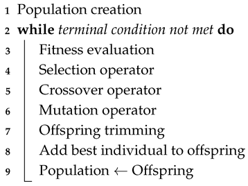
The algorithm begins with the standard GA with elitism, as presented in Algorithm 1. This version serves as the foundation for the quantum–classical evolutionary optimization algorithm introduced later, and also provides a reference for performance comparison. The operators used are well-known and commonly applied, specifically tournament selection, heuristic crossover, and uniform mutation. These operators are detailed in Algorithms 2, 3, and 4 respectively.
| Algorithm 1: Genetic algorithm. |
![Applsci 15 08029 i001]() |
Trimming the offspring may be necessary because the number of generated offspring does not always equal the original population size. This trimming process involves randomly selecting a number of offspring to match the population size. Next, the best individual from the previous generation is inserted into the offspring population by replacing a random individual. This introduces elitism, which has been shown to improve GA performance in various scenarios [
12].
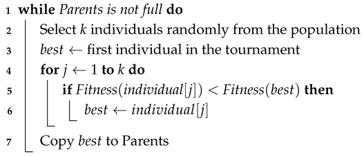
| Algorithm 2: Tournament selection operator. |
![Applsci 15 08029 i002]() |
Tournament selection forms random pools to reduce the likelihood of always selecting the best individual as a parent. This increases genetic diversity without sacrificing selection pressure. However, this method can lead to multiple copies of the same individual being selected, which may increase the risk of population stagnation.
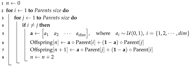
| Algorithm 3: Heuristic crossover operator. |
![Applsci 15 08029 i003]() |
Heuristic crossover is a simple yet effective method that ensures all offspring are generated along the line segments connecting parent pairs. It is especially useful in convex problems or non-convex problems, where the minimum is surrounded by several local minima. However, it lacks strong exploratory capability.
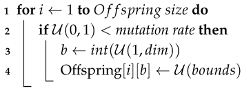
| Algorithm 4: Uniform mutation operator. |
![Applsci 15 08029 i004]() |
When an individual is selected for mutation, the uniform mutation operator randomly reassigns one of its genes with a new value, uniformly drawn from within the search space. The uniform probability density function (PDF) enhances exploratory capabilities in the early generations, but it reduces convergence speed as the population nears the optimum.
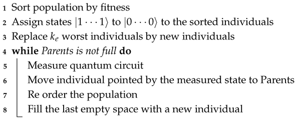
In GAQS, the tournament selection operator is replaced by a hybrid quantum–classical selection operator called the quantum selection operator (QSO), presented in Algorithm 5. This operator first sorts the population by fitness and assigns quantum states ranging from
to
to each individual. This mapping links individuals with quantum states. Next, the
worst individuals are removed and replaced with new random individuals. This step boosts genetic diversity in the population.
| Algorithm 5: Quantum selection operator. |
![Applsci 15 08029 i005]() |
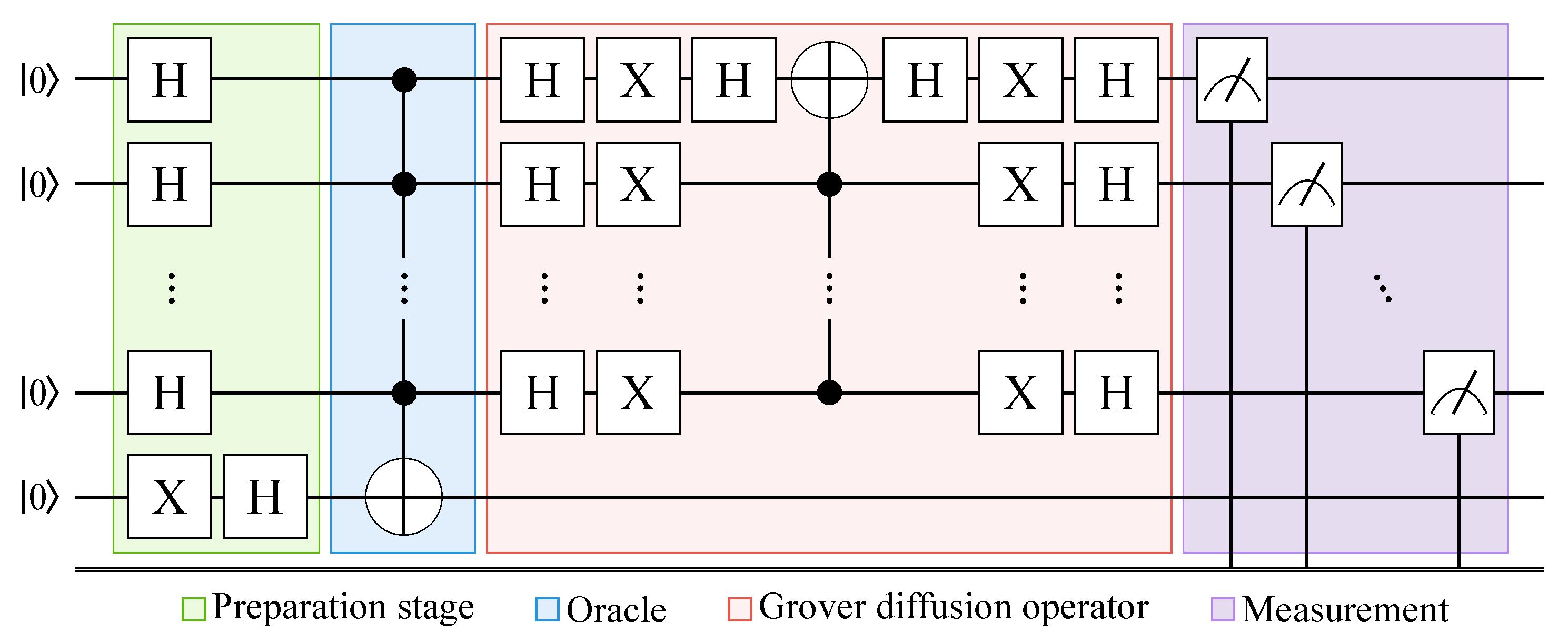
Parent selection proceeds by measuring a quantum circuit (QC), which determines which individual is selected as a parent. The selected individual is added to the parent pool, and the population is re-sorted. A new individual is then added to replace the removed one, maintaining diversity. Unlike tournament selection, this process avoids duplicating individuals, which helps prevent stagnation.
The QC used in QSO is shown in
Figure 1. It is an amplitude amplification circuit of
n qubits consisting of 4 sections [
13]. Amplitude amplification is a quantum computing mechanism for enhancing the probability of measuring a desired outcome. In this case, the desired outcome is the quantum states related to the individuals with the best fitness, effectively weighting the selection towards them.
Each one of the sections in the amplitude amplification plays a crucial part in the final outcome and can be seen as a step-by-step process. The first section is the preparation stage; it works by creating a uniform superposition of all the states in the quantum circuit. When all states are in uniform superposition, all have the same probability of being measured.
The second step is performed by the oracle; it is a small QC that has the most important role. It marks the states that are to be amplified using a rotation. It works by checking all present states in parallel and applying a controlled rotation only to the states that are desired. In the case of the QC previously presented, the oracle is a multicontrolled X-gate. This gate applies a rotation of on the X axis of its target qubit (the qubit with the white circle with the plus inside) when all its inputs (the qubits with the small black dots) are in the state |1〉. Since all the states in the quantum circuit are in uniform superposition, what the oracle does in this case is not modify any state except for the state to which it applies the rotation.
The status of the states after the oracle is that all have a positive amplitude but the state , which has a negative one. However, all of them have the same absolute value. The third step is performed by the Grover diffusion operator (GDO); this is a complex quantum circuit, but its working principle is simple. It takes the mean value of the amplitudes of all the states and rotates them around it. In the case of the QC presented in the figure, the mean value of the amplitudes is positive. When all the states are rotated around it, the final outcome is that all states with positive amplitude suffer a decrease in their amplitudes’ absolute value, while the state (the only one with negative amplitude) has its absolute value increased, resulting in the state having the highest amplitude’s absolute value.
The final step is the measurement, the measurement of a quantum circuit is stochastic in nature. The probability of measuring a state is given by the square of the absolute value of the state’s amplitude. Taking into account the way in which the amplitudes of the states are after the GDO, it is easy to understand that the state (which is related to the best individual) is more expected to be measured, applying in this way a strong selection pressure on selecting the fittest individuals.
3. Genetic Algorithm with Quantum Selection and Simulated Binary Crossover
After achieving promising initial results with GAQS on EM problems [
11,
14], a further improvement was proposed in [
15]. This enhancement involves replacing the crossover and mutation operators with more sophisticated classical ones, specifically, simulated binary crossover (SBX) and Gaussian mutation. These are presented in Algorithms 6 and 7.
| Algorithm 6: Simulated binary crossover operator. |
![Applsci 15 08029 i006]() |
| Algorithm 7: Gaussian mutation operator. |
![Applsci 15 08029 i007]() |
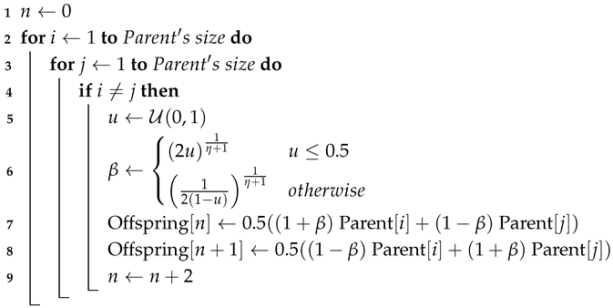
SBX was introduced in [
16] and replicates, for real-valued genes, the behavior of one-point binary crossover. Offspring are generated along the line segment connecting each pair of parents and are distributed according to a probability density function that resembles the sum of two Gaussian PDFs centered at the parents’ positions. This distribution grants the operator strong exploratory capabilities but results in increased computational cost and reduced performance near the minimum, where problems tend to be approximately convex. The parameter
controls the concentration of offspring around their parents.
Gaussian mutation operates similarly to uniform mutation, with the key difference being that the mutation value is drawn from a Gaussian distribution rather than a uniform one. The distribution is centered on the gene’s current value, and the standard deviation determines the spread of the mutated values.
In this setup, the weaknesses of SBX (which performs poorly near optima) are mitigated by the strength of the Gaussian mutation (which is better suited for local fine-tuning), and vice versa. This complementary relationship yields a more flexible algorithm than the one presented in
Section 2. Specifically, the two additional parameters
and
provide fine control over exploration and exploitation. The version of GAQS that incorporates SBX and Gaussian mutation is referred to as GAQS SBX.
4. Mathematical Test Functions
For testing optimization algorithms, it is common to use mathematical functions with known analytical results that are generalized to N dimensions. When applied in this context, they are usually referred to as mathematical test functions (MTFs) or mathematical benchmarks. They can be classified into two groups: convex and non-convex MTFs. Convex MTFs have one minimum and are easy to solve using classical non-evolutionary algorithms, but are somewhat challenging for evolutionary algorithms with strong exploratory capacities.
On the other hand, non-convex MTFs have multiple local minima and local maxima, making non-evolutionary optimization algorithms unreliable, and have been proven challenging for evolutionary algorithms that lack exploration capacities. The use of MTFs evaluates the resistance to stagnation of optimization algorithms, exposing the need for increasing the exploratory capacity of the algorithm. The considered MTFs for this paper are presented in
Table 1.
The Manhattan norm is a compact and easy-to-compute function that has some complexity even while being convex. Its complexity is given by the discontinuities in
, which cause it to be non-differentiable over its whole domain. It was selected due to its low computational complexity and simplicity of implementation. It is plotted in two dimensions in
Figure 2a.
The Rastrigin and Griewank functions are two non-convex MTFs. Both have multiple local minima and local maxima. However, Griewank has more critical points in the considered bounds. On the other hand, the rate of change in the structure of the function is lower in Rastrigin, making its local minima harder to distinguish for the algorithm.
Both functions are challenging for optimization algorithms due to their irregular nature. It is common to use them in conjunction because their differences help to highlight the weaknesses in optimization algorithms. Both functions are plotted in two dimensions and presented in
Figure 2b,c.
5. Electromagnetic Design Problems Considered
In this paper, two electromagnetic design problems (EMDPs) are considered. The first one is the design of a wideband microstrip filter, and the second one is the design of a multilayer EM absorber.
These EMDPs are commonly encountered in telecommunications. The design of filters is crucial in the development of RF front-ends, as they reject unwanted harmonic distortion introduced by nonlinearities in amplifiers, as well as unwanted intermodulation products produced by mixers. On the other hand, EM absorbers are used in anechoic chambers as a tool to eliminate reflections and external noise. In this way, an ideal line-of-sight condition can be emulated, which is crucial for the correct characterization of antennas for telecommunications and the study of electromagnetic compatibility in consumer electronics.
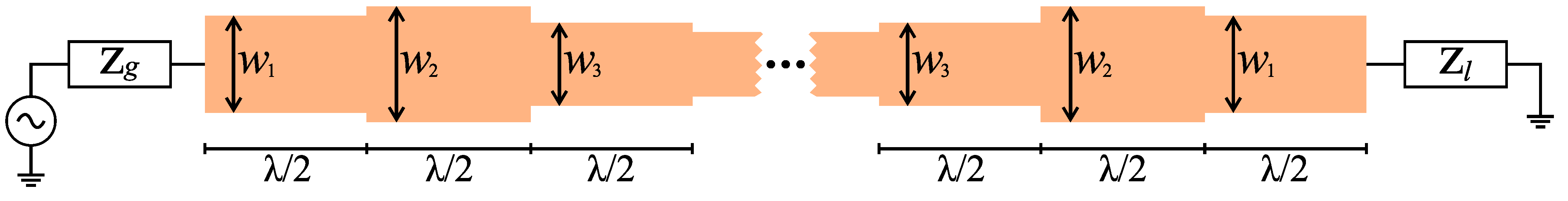
5.1. Wideband Microstrip Filter
For the design of the filter, a set of
pieces of transmission line connected in a series is used. The filter is symmetric, meaning that the first and last pieces are equal, the second and second-to-last pieces are equal, and so on. In this way, only
N variables are necessary to represent the whole circuit. The structure of this filter is presented in
Figure 3.
The filter behavior is well described by the transmission lines theory presented in [
17,
18]. The
parameters of this device are obtained by using its transmission matrices, the load impedance
, and the source impedance
as shown in the following equation:
As hinted before, the variables used in the optimization are the widths of the first N pieces of the filter. The fitness function is then computed as a weighted sum of the following parameters:
Mean of the in-band ripple;
Maximum in-band ripple;
Violation of the out-of-band mask;
at ;
Penalization for bandwidth smaller than .
The mask is set symmetrically with respect to
, starting at 0 dB at
and descending 30 dB per
. The out-of-band violation is computed by taking the difference between the
of the filter and the mask, then taking the integral of the positive intervals of this subtraction. This process is better explained using the following equation:
The central frequency and filter dimensions are expressed in terms of and . This indicates that the filter design is general and can be used in any desired frequency compatible with microstrip technology for the available substrates.
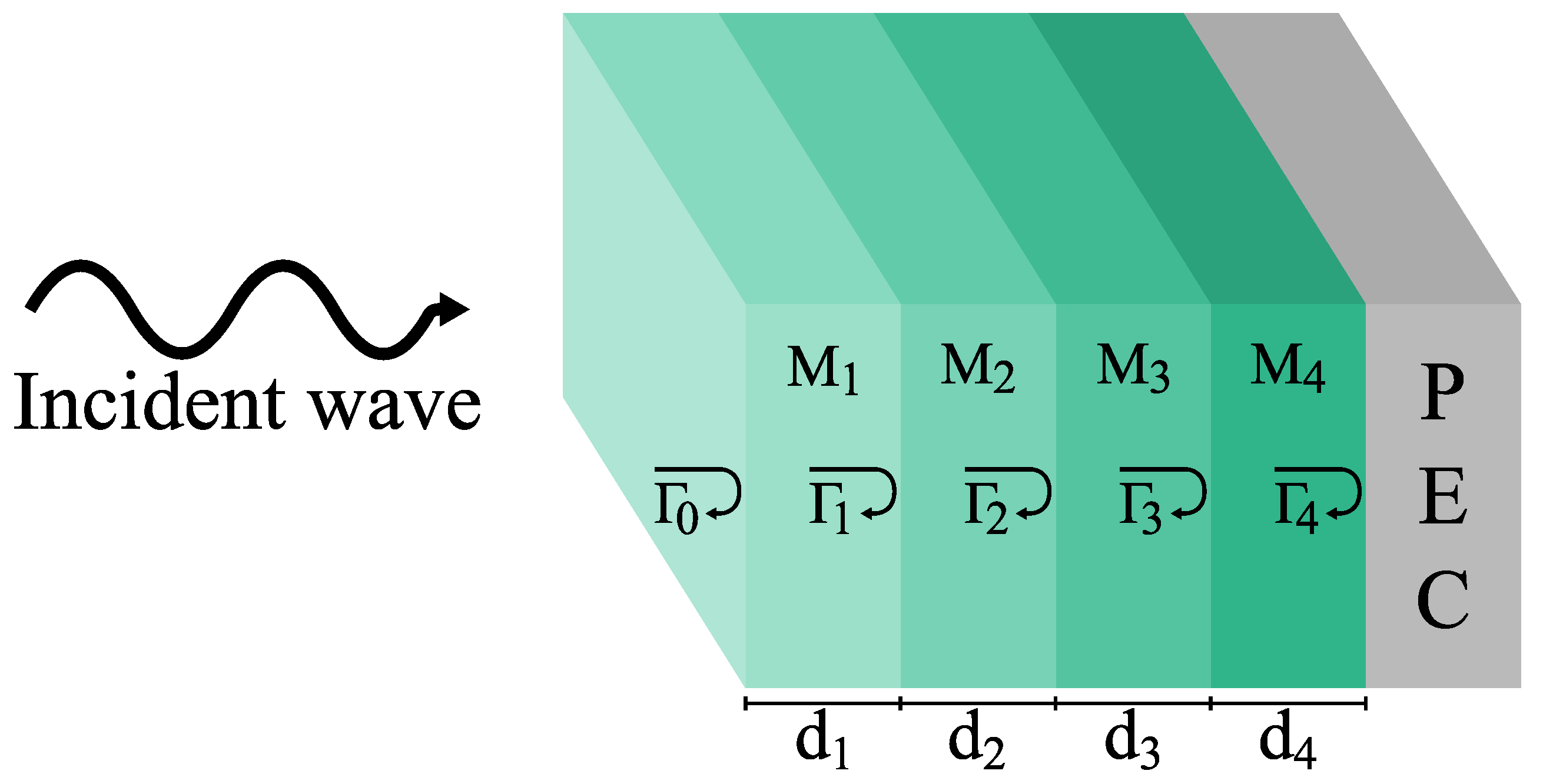
5.2. Multilayer EM Absorber
A multilayer EM absorber is a stack of
N materials as shown in
Figure 4. The materials that are used are lossy, dissipating the power transported by the EM wave into thermal energy, thereby reducing the reflected power. The thickness of each layer plays an important role not only in the effective impedance perceived by the incoming EM wave. However, in many applications, the total thickness of the absorber has to be as low as possible to reduce the overall occupied space or to keep its weight below a given constraint.
For this problem, normal incidence is considered for the incoming EM wave; additionally, all the materials are considered purely dielectric, lossy, and non-frequency selective (
,
, and
). The reflection coefficient for normal incidence [
19] can be approximated as
Considering the values of
in the first layers to be low,
and
are computed using the following equations:
The fitness function is computed as a weighted sum between the mean value of the reflection coefficient in the target band
and the total thickness of the absorber. The final design is the combination of slab thicknesses that achieves the trade-off between total thickness and absorption dictated by the weight
w.
6. Materials and Methods
All the results presented in
Section 7 were obtained using a laptop with an Intel Core i7 10710U CPU, an Nvidia GTX 1650 GPU, and 16 GB of RAM. All algorithms were implemented with Python 3.11, Numpy 1.23, and Scipy 1.14. For GAQS and GAQS SBX, the QC measurements were not done during the execution of the code, but a pool of (more than 10,000) measurements was created beforehand and used in all the executions after being shuffled. The measurements were done using two approaches. The first one used the Aer simulator available as a sub-library in Qiskit (Qiskit-aer 0.12.1).
The second one used IBM-Sheerbroke, a real quantum computer equipped with the Eagle r3 quantum processor. The connection to the IBM quantum platform had to be done using the latest versions of Qiskit and qiskit-ibm-runtime. When using IBM’s quantum computers, the circuit has to be transpiled to accommodate the architecture of the quantum processor.
The use of a pool of measurements is motivated by the long queues that can be encountered when connecting to IBM quantum computers due to their free and easy access. The algorithms use the parameters presented in
Table 2.
All MTFs were executed with 4 dimensions, the wideband filter was tested with N = 9 and center frequency
, and the EM absorber used 4 layers of purely dielectric lossy materials with permittivity presented in
Table 3. The weight
w was set to 50, the thicknesses of the materials are considered in mm, and the target bandwidth was 2 to 6 GHz. This covers the 2.4 GHz and 5 GHz bands used in most commercial communications systems such as WiFi and Bluetooth, as well as the majority of the non-millimeter wave bands used for cellular telephony in 4G and 5G [
20].
The materials used are fictitious, as the characterization of real materials is outside the scope of this paper. All the tests presented were conducted 200 times, with 200 generations each, to allow for a statistical analysis of the final results and to prevent incorrect conclusions caused by outliers.
7. Results and Discussion
The results and analysis presented hereafter are divided into four subsections. Each test was done for the three considered algorithms, following the considerations previously stated in
Section 6. The
Section 7.1 presents and analyzes the behavior of the evolution of the mean value of all the tests done per algorithm.
The
Section 7.2 presents and analyzes the convergence speed through the square root of the rate of change of the mean value of the fitness (SRMF). The square root was used to improve the visualization of the data, as the use of a logarithmic scale was discarded due to the presence of zero values. In addition, a moving average (MA) of SRMF was taken with a window of 10 samples. Its aim was to reduce the visual impact of the fluctuations of SRMF and therefore provide a clearer image of each algorithm’s performance.
The
Section 7.3 presents the statistics of the final results of the tests in a box plot. This representation presents all the information in a compact format and allows for an easy comparison between the different algorithms tested.
In the
Section 7.4, the Wilcoxon signed-rank test was performed on the final results obtained from all optimization runs to evaluate the hypothesis generated in the three previous subsections.
Finally, in the
Section 7.5, the average time per generation is presented. It aims to show the difference in computational complexity between the algorithms, as well as the impact that the fitness function computation has on the overall execution time.
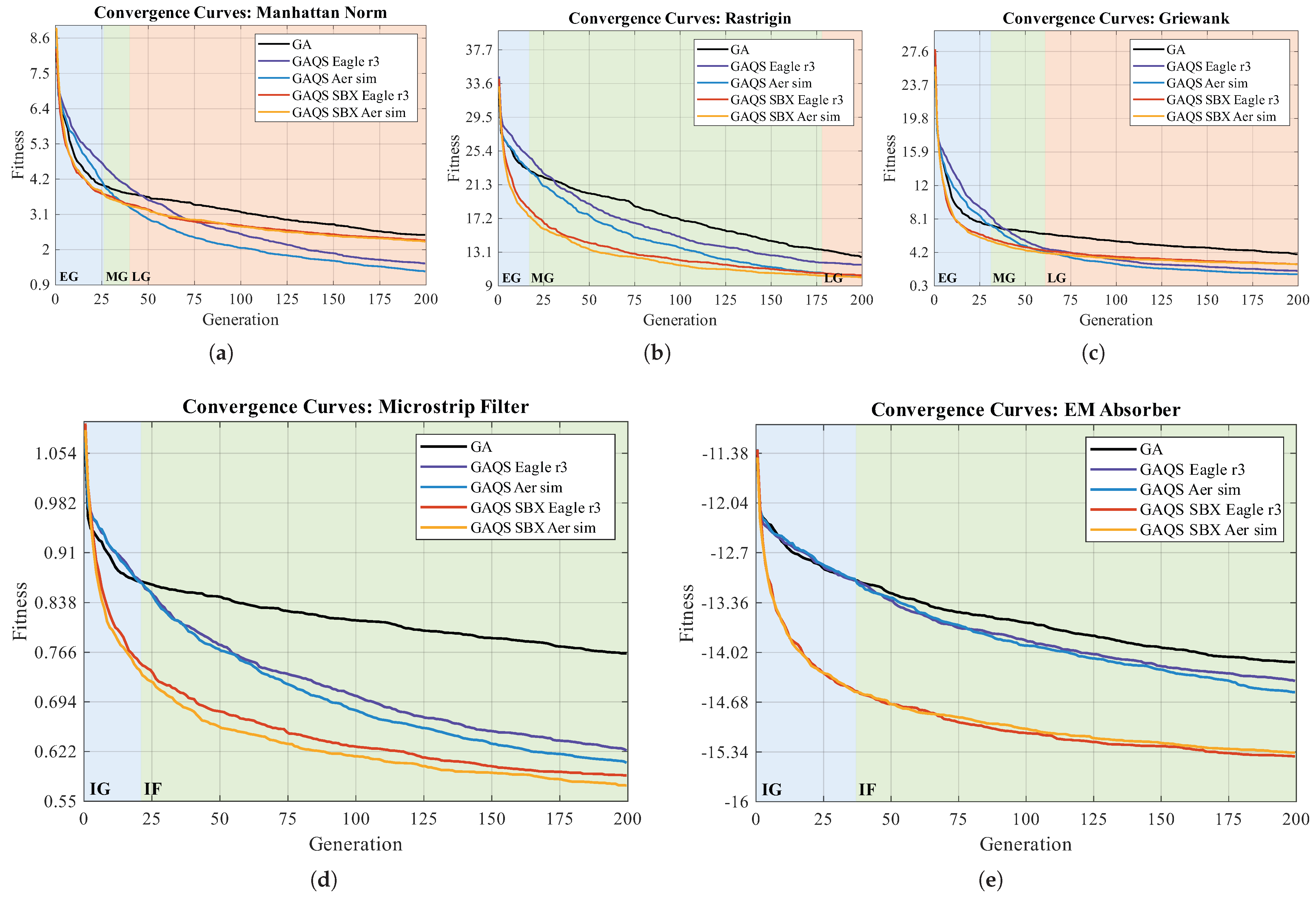
7.1. Fitness’s Mean Value Evolution
The mean value evolution per algorithm is presented in
Figure 5 for all the considered tests. In general, for the MTF (
Figure 5a–c), three distinct regions can be defined using the differences between the fitness values of the algorithms. The first region, called early generations (EGs), goes from generation 1 until GAQS surpasses GA. The second region, middle generations (MGs), goes from GAQS surpassing GA to GAQS equaling GAQS SBX. The last region, called late generations (LGs), goes from GAQS equaling GAQS SBX onward. In simple equations,
Early generations (EGs): ;
Middle generations (MGs): ;
Late generations (LGs): .
In EG, the mechanisms introduced in GAQS for increasing genetic diversity slow down the initial evolution of the algorithm compared to GA. However, the strong exploratory characteristics of SBX overcome the initial slowness of QSO, giving GAQS SBX the best overall performance.
In MG, the higher genetic diversity conferred by QCO in GAQS eventually overcomes GA. However, due to the convex nature of the Manhattan norm and the central minimum in all considered non-convex MTFs, heuristic crossover starts to perform better than SBX until GAQS surpasses GAQS SBX.
In LG, the advantage of the heuristic crossover becomes clear as SBX causes a decrease in the convergence speed. Moreover, the measuring method’s impact is problem-dependent. Overall, quantum computers are slower than Aer simulators, and noisy measurements worsen GAQS SBX performance, especially in EG. The timing of EG, MG, and LG depends entirely on the MTF.
For the EMDP, only two regions can be observed: initial generations (IGs) and final generations (FGs). They are equivalent to EG and MG and they are defined as
Due to the low number of generations, LG is not observed. It might appear in future generations near the minimum, where performance converges. Thus, GAQS may eventually outperform GAQS SBX.
For the microstip filter in
Figure 5d, the IG shows fast convergence for GAQS SBX due to its strong exploratory capacity, GA stagnates after generation 25, and in FG, GAQS SBX shows rapid improvement followed by GAQS; after generation 100, GAQS SBX slows down.
On the other hand, GA tends to stagnate after generation 25 (see
Appendix A), negatively affecting its performance. The difference between the Aer simulator and the quantum computer measurements is noticeable in both versions of GAQS, especially in FG. It suggests that the stronger selection pressure due to the obtained noiseless measurements from the Aer simulator are favorable for this problem.
For the EM absorber in
Figure 5e, IG is harder to define but occurs when GAQS starts outperforming GA, FG shows GAQS SBX leading again due to higher genetic diversity, and GAQS SBX continues to perform well in FG, though it slightly deteriorates post-generation 100.
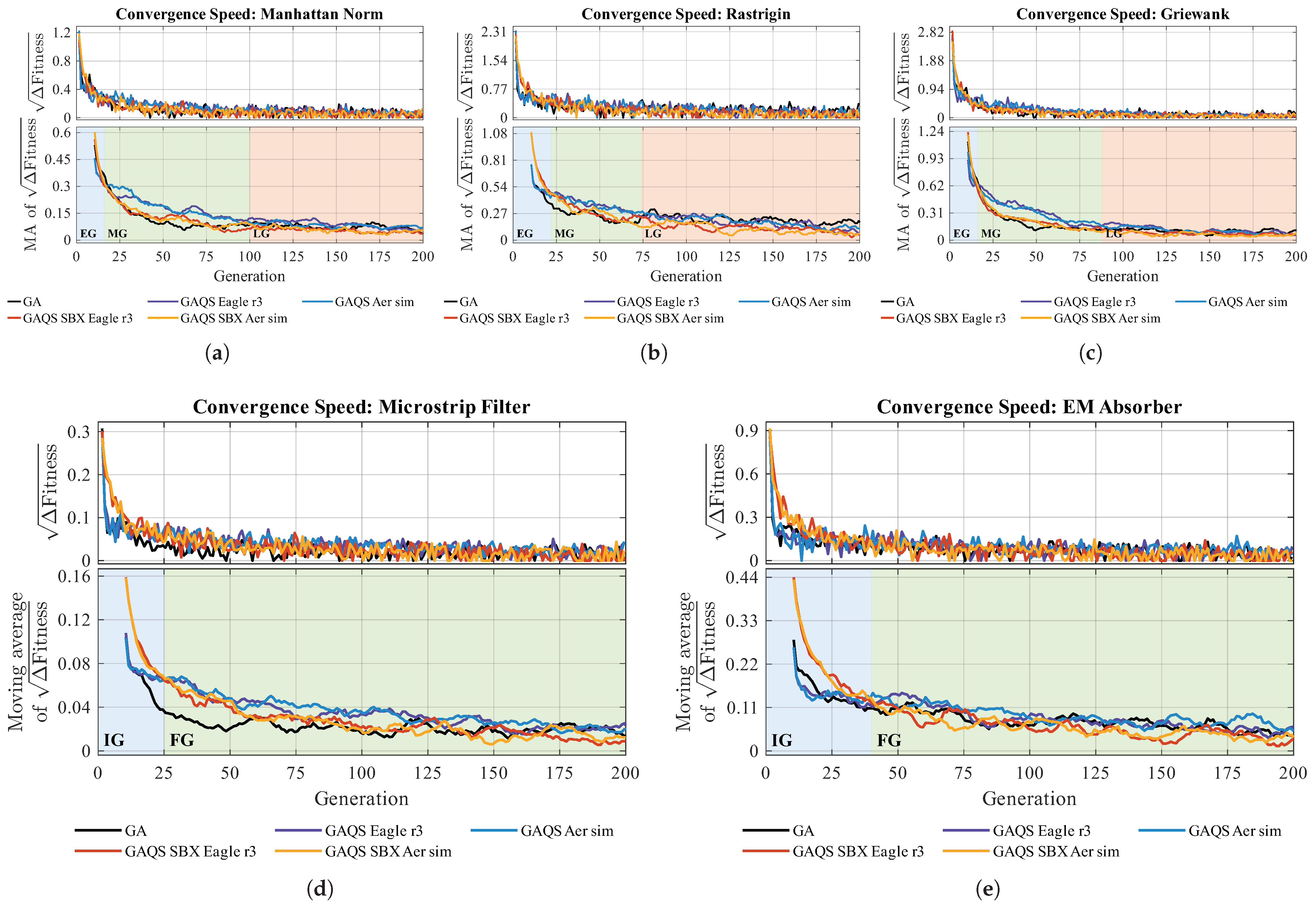
7.2. Convergence Speed
The convergence speed represented by the SRMF is shown in
Figure 6 as well as its MA obtained as explained in the
Section 7.1. Since the SRMF fluctuates too quickly, the discussion of the results is focused on the MA. For the MTF, three regions are present again. They are described as follows:
Early generations (EGs): ;
Middle generations (MGs):
;
Late generations (LGs):
.
In EG, the observed behavior and the reasoning behind it are the same as the ones presented in
Section 7.1. In MG, the MA of SRMF provides more information on the behavior observed before. The way GAQS catches up with GA and GAQS SBX in fitness is clearly explained by GAQS having a slower convergence speed in the beginning but keeping it higher for longer. On the other hand, GA and GAQS SBX start to decelerate only after a few generations. This behavior can be explained by the higher genetic diversity offered by QCO and a decrease in the performance of SBX after the initial exploration.
In LG, the decrease in performance is even more noticeable when GA starts to outperform GAQS SBX in convergence speed. The decrease in performance of SBX is caused by excessive search outside the boundaries set by the parents and an increase in the performance of HCO near the minimum in the MTF. Once again, the moment when the regions appear is completely problem-dependent.
For the EMDP only two regions are clearly distinguishable. However, their characteristics vary with respect to the MTF and they are defined as
For both EMDPs, the IG is marked by a clear difference in the initial convergence speed between GAQS SBX and the other algorithms. This is a showcase of the positive impact of SBX in early generations, where its search capacities are fully exploited.
For the microwave filter in FG, the search capacity of SBX becomes counterproductive after some generations when the heuristic crossover starts to explore the region delimited by the parents more efficiently. Nonetheless, the convergence speed of GAQS SBX is still higher than that of GA due to the resistance to stagnation offered by QSO.
On the other hand, in FG for the EM absorber, GAQS SBX has on average the slowest convergence speed, but the overhead in fitness obtained in IG is too significant, explaining its decline with respect to GA. Nonetheless, GAQS keeps a higher convergence speed than GA, showcasing the advantage of keeping a higher genetic diversity to both convergence speed and resistance to stagnation.
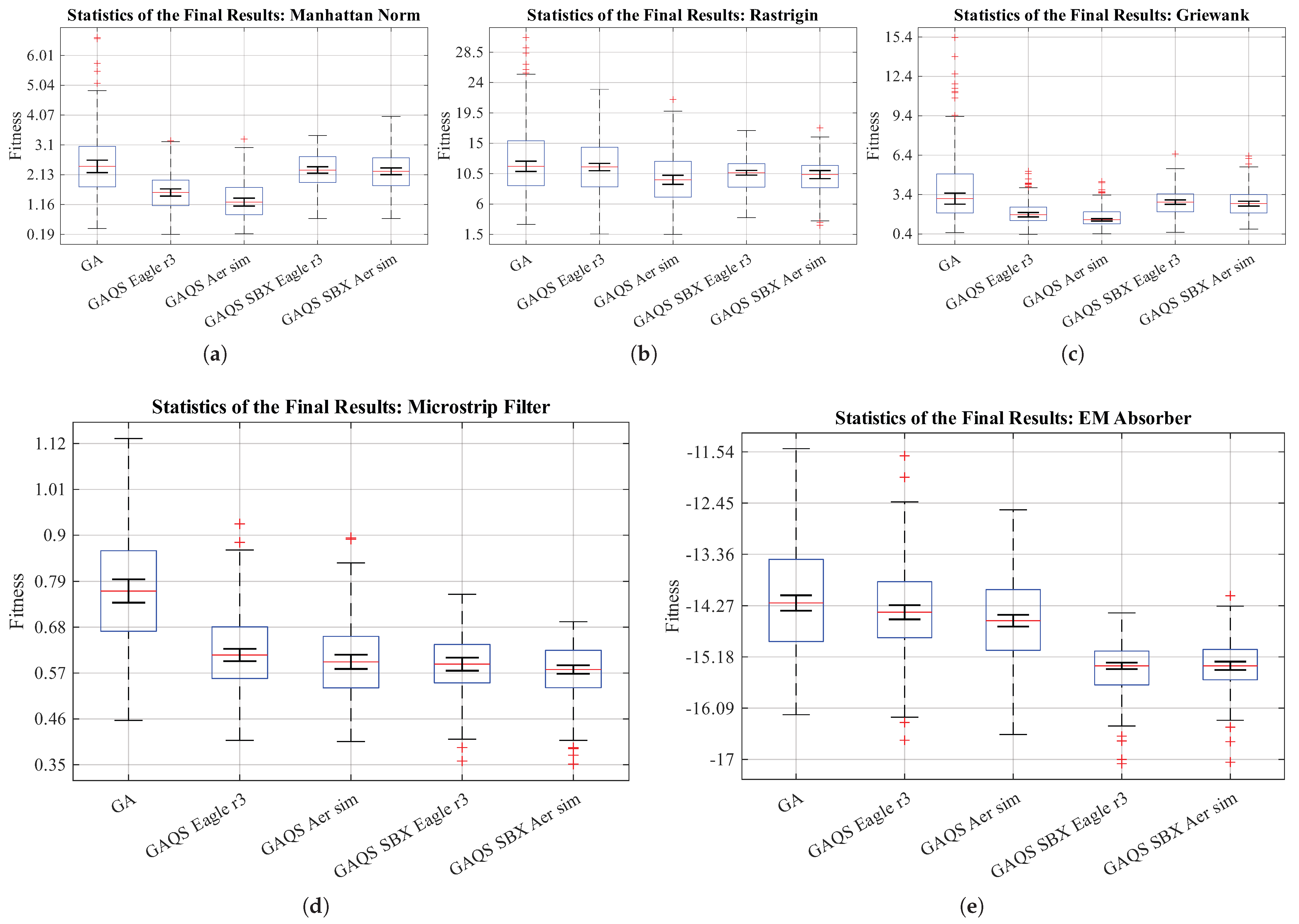
7.3. Final Results Statistics
The statistics of the final results for all the tests are presented as box plots in
Figure 7. A box plot is a simple plot that allows the visualization of the results of an experiment in a concise way. Its four main parts have the following interpretation in the context of an evolutionary optimization algorithm:
Median: It is the red line inside the box; it is similar to the mean, which has already been interpreted in the previous subsections. Its 95 % confidence interval is given by the black lines above and below it.
Interquartile range (IQR): It is a box that represents the distance between the first and third quartiles of the data. Its interpretation is linked to the repeatability of the results. A smaller IQR means that the algorithm is less inclined to have an unexpected behavior. On the other hand, a large IQR makes the algorithm less reliable on a single run.
Whiskers: They contain all the data 1.5 IQR in distance from the box. In this case, their interpretation is the same as the IQR.
Outliers: They are all the data not contained in the whiskers; in this work, all outliers are preserved. Depending on their position, they have the following interpretation:
- –
High-fitness outlier: If there are many, they suggest that the algorithm has a tendency to have low-performing executions, usually due to stagnation.
- –
Low-fitness outlier: If there are many, they suggest that the algorithm has a tendency to have higher-than-average performing executions.
In every case, the performance of both versions of GAQS outperforms GA in both median and IQR, making them a more reliable option. Furthermore, the presence of high-fitness outliers is almost exclusive of GA, except for the test done with the Griewank function in GAQS. Moreover, the presence of low-fitness outliers is limited to GAQS SBX, showing that the strong exploration of SBX may result in flukes. However, these are not representative of the real performance of the algorithm.
The best-performing algorithm is problem-dependent. Nonetheless, for MTFs, GAQS is more likely to be the best, while for the considered EMDP, GAQS SBX is more likely to be the best. In any case, the algorithm with the best performance in terms of median is usually the best algorithm in IQR too. Furthermore, the IQR is independent of the measuring methodology used, while the median is affected by it.
7.4. Wilcoxon Signed-Rank Test
In the previous three subsections, two main hypotheses were raised, the first one was that GAQS and GAQS SBX outperform GA on all problems evaluated. The second was that, in general, when GAQS and GAQS SBX use measurements obtained from the Aer simulator, they outperform themselves when using measurements obtained from the Eagle r3 quantum processor.
To test these hypotheses, the Wilcoxon signed-rank test was performed. The results are presented in
Table 4; the hypothesis is confirmed when the value of p recorded in the table is smaller than 0.05. Considering what was previously stated, it is confirmed that GAQS and GAQS SBX significantly outperform GA. However, the hypothesis that when the algorithms use the Aer simulator, they significantly outperform themselves when using Eagle r3 is not true in all cases. It holds true for GAQS in all cases but one (which is borderline), but it does not hold for GAQS (again, in all cases but one). It suggests that the measurement fidelity significance decreases with the quick initial boost in convergence speed given by SBX.
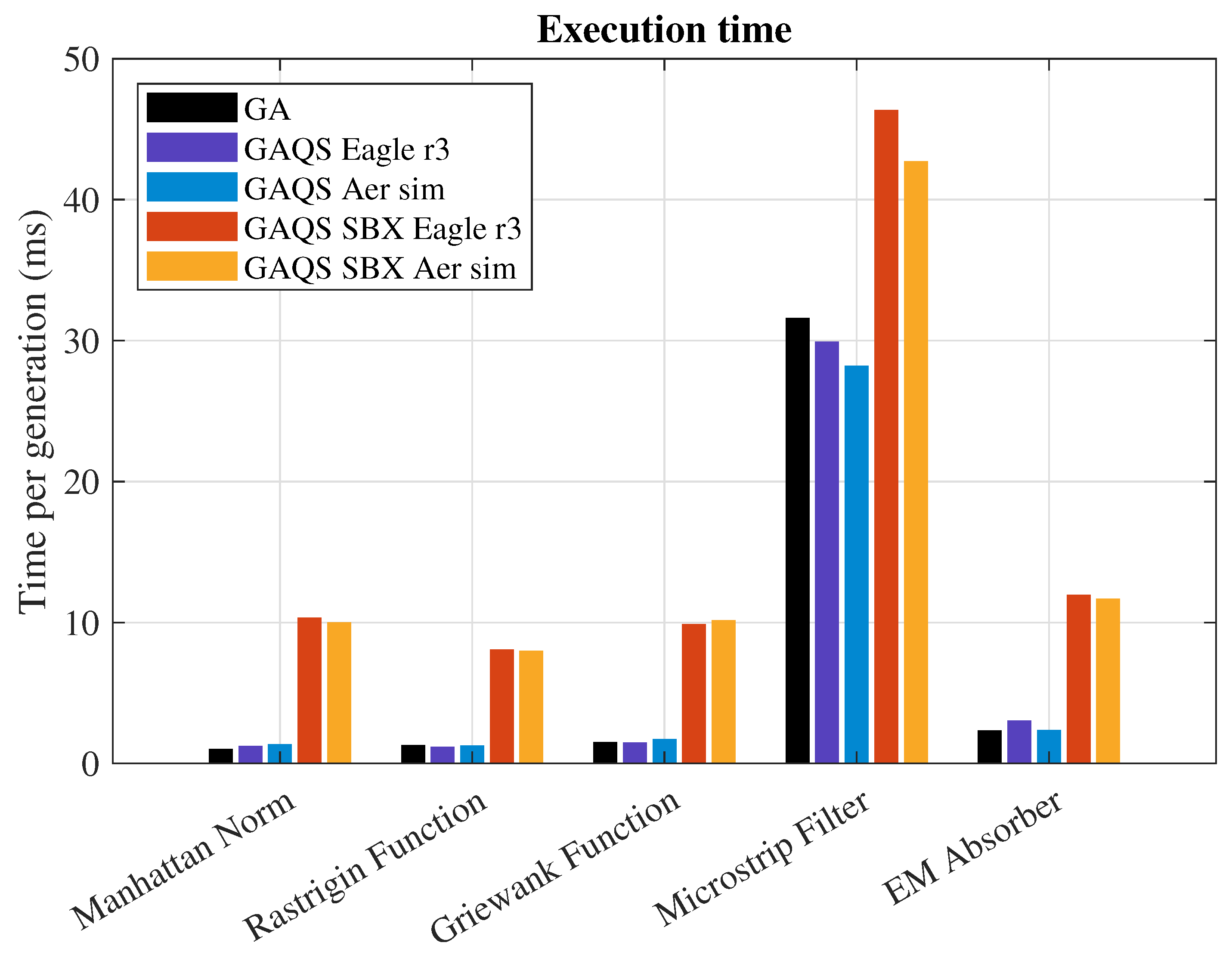
7.5. Average Time per Generation
Figure 8 presents the average time per generation of each one of the algorithms in the tests considered. Since the laptop used for the tests had multiple pieces of software installed and some of them may have been running in the background or looking for updates, the times cannot be considered as the absolute truth. But, they can still give an idea of the behavior of the algorithms.
It is observed that GA and GAQS take approximately the same time per generation, showing that using the pool method for the measurements gives an extraordinary advantage with respect to doing the simulations or measurements while running the code. Moreover, the measuring method has no impact on the computation time, once again due to the pre-measuring technique. In the future, the measurements could be done in parallel so that the computational time would not be increased.
GAQS SBX takes considerably more time to run than GAQS due to the substitution of heuristic crossover by SBX. Nonetheless, the impact of these increases can be neglected when the evaluation of the fitness function takes much longer than the execution of the optimization algorithm in itself. This effect is noticed for the microstrip filter.
8. Conclusions
The results previously presented showed the superiority of QSO over traditional selection operators in convex MTFs, non-convex MTFs, and the EMDP considered. GAQS and GAQS SBX have been tailored to achieve great results in the EMDP by boosting the diversity of the population and, with it, increasing its resistance to stagnation. However, due to the NFL theorem, its performance may not be as good with other types of problems. Nonetheless, the positive results obtained with the MTFs suggest a great domain of applicability, especially in problems where classical algorithms have the tendency to stagnate.
The flexibility present in GAQS and GAQS SBX, given by the fact that they are a sort of modified GA, gives the possibility to apply them to any problem where evolutionary algorithms have been previously applied. Furthermore, considering that they work with a population, they can be migrated from single-objective optimization to multi-objective optimization by correctly defining a fitness function in terms of domination and diversity.
The appearance of regions in the evolution of the algorithms is also a clear indication that GAQS can be further improved by combining the exploratory capacities of SBX and the deep search of heuristic crossover. However, additional studies on this topic have to be conducted. Finally, this paper focuses on the analysis of the behavior of algorithms rather than on the design of the EM devices themselves. To observe some of the devices designed with GAQS, it is suggested to check [
14,
15,
21].
This work has demonstrated that the GAQS and GAQS SBX algorithms can be applied effectively to single-objective optimization in electromagnetic design. However, some engineering problems are better addressed as multi-objective problems. Since GAQS is a population-based algorithm, expanding it to a multi-objective optimization (MOO) is possible.
In MMO, the concept of a single fitness value is replaced by the concept of Pareto dominance and diversity in the Pareto front. Since QSO assumes a scalar fitness metric for sorting and mapping quantum states, it can be modified to sort and map the quantum states based on sets of individuals that belong to the same non-dominated front, sorting the individuals in the same group based on their spacing. Moreover, changes to the oracle are to be expected in this context to reduce the selection pressure and boost diversity. Based on the results obtained in single-objective optimization, it is expected that with adequate modifications, QSO can be a successful operator in MMO algorithms.
Author Contributions
Conceptualization, G.F.M. and R.E.Z.; methodology, G.F.M., A.N., and R.E.Z.; software, G.F.M. and A.N.; validation, G.F.M., A.N., and R.E.Z.; formal analysis, G.F.M. and R.E.Z.; investigation, G.F.M.; resources, G.F.M., A.N., and R.E.Z.; data curation, G.F.M.; writing—original draft preparation, G.F.M. and E.L.Z.; writing—review and editing, G.F.M., E.L.Z., and R.E.Z.; visualization, G.F.M. and E.L.Z.; supervision, A.N. and R.E.Z.; project administration, R.E.Z.; funding acquisition, R.E.Z. All authors have read and agreed to the published version of the manuscript.
Funding
This study was carried out within the project SMARTEYE and received funding from the Ministero delle Imprese e del Made in Italy (Prog n. F/310276/03/X56). This manuscript reflects only the authors’ views and opinions.
Institutional Review Board Statement
Not applicable.
Informed Consent Statement
Not applicable.
Data Availability Statement
The dataset obtained from all the optimization runs is available in doi:10.5281/zenodo.15756231. Further inquiries can be directed to the corresponding author.
Acknowledgments
We thank Marco Mussetta for the discussions that added value to this research as well as to the student of the bachelor in Aerospace engineering at Politecnico di Milano whose questions help us enrich our work. We acknowledge the use of IBM Quantum platform for this work.
Conflicts of Interest
The authors declare no conflicts of interest.
Abbreviations
The following abbreviations are used in this manuscript:
| BCE | Before common era |
| EA | Evolutionary optimization |
| EGs | Early generations |
| EM | Electromagnetic |
| EMDP | Electromagnetic design problem |
| FGs | Final generations |
| GA | Genetic algorithm |
| GAQS | Genetic algorithm with quantum selection, heuristic crossover and uniform mutation |
| GAQS SBX | Genetic algorithm with quantum selection, simulated binary crossover and |
| Gaussian mutation |
| GDO | Grover diffusion operator |
| IGs | Initial generations |
| IQR | Interquartile range |
| LGs | Late generations |
| MA | Moving average |
| MGs | Middle generations |
| MTF | Mathematical test function |
| NISQ | Noisy intermediate-size quantum |
| PDF | Probability density function |
| PSO | Particle swarm optimization |
| QAOA | Quantum approximate optimization algorithm |
| QC | Quantum circuit |
| QSO | Quantum selection operator |
| SBX | Simulated binary crossover |
| SRMF | Square root of the rate of change of the mean of the fitness |
| Randomly generated number with uniform PDF distributed between a and b |
| Randomly generated number with gaussian PDF with mean and standard |
| | deviation |
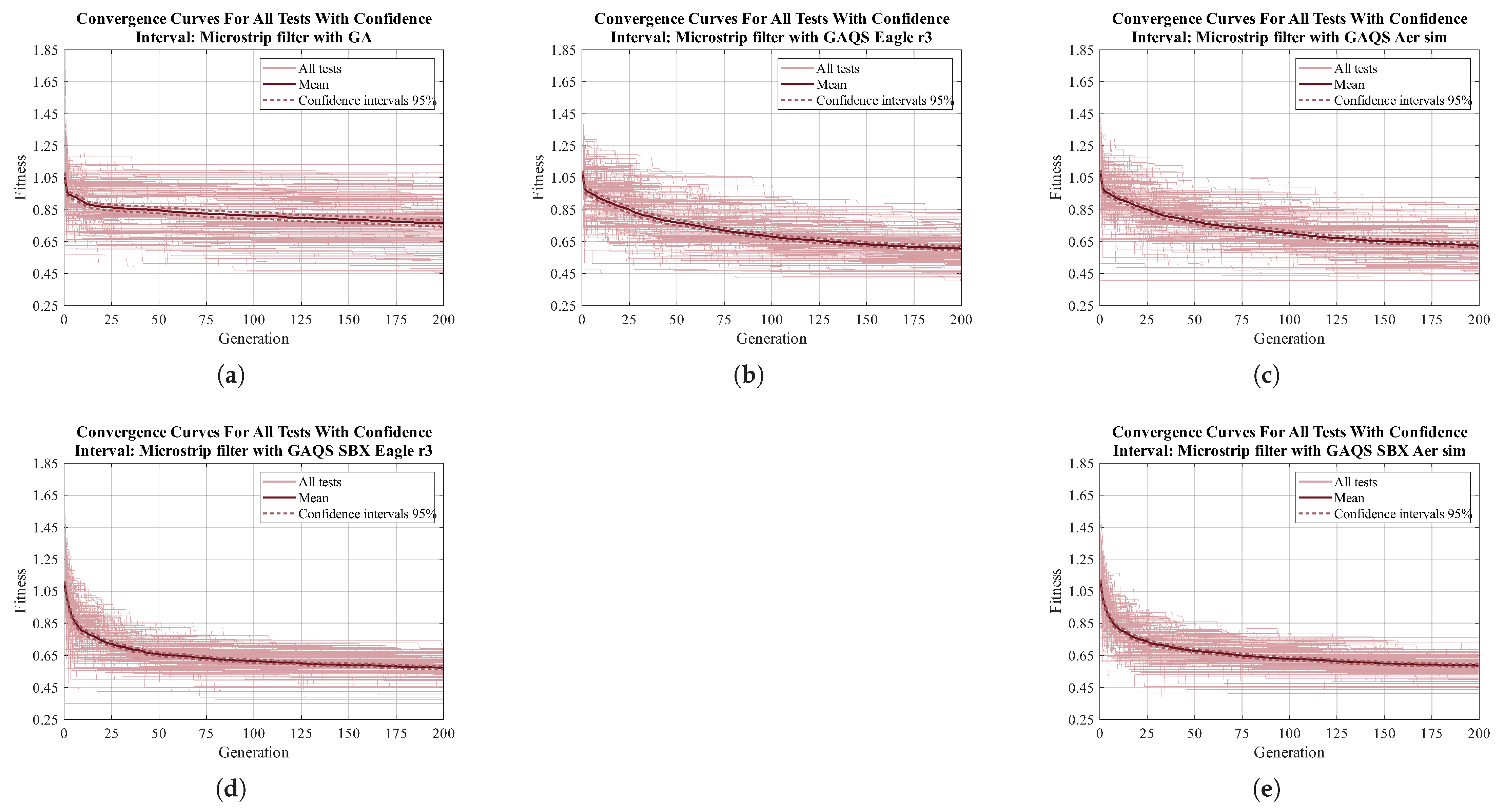
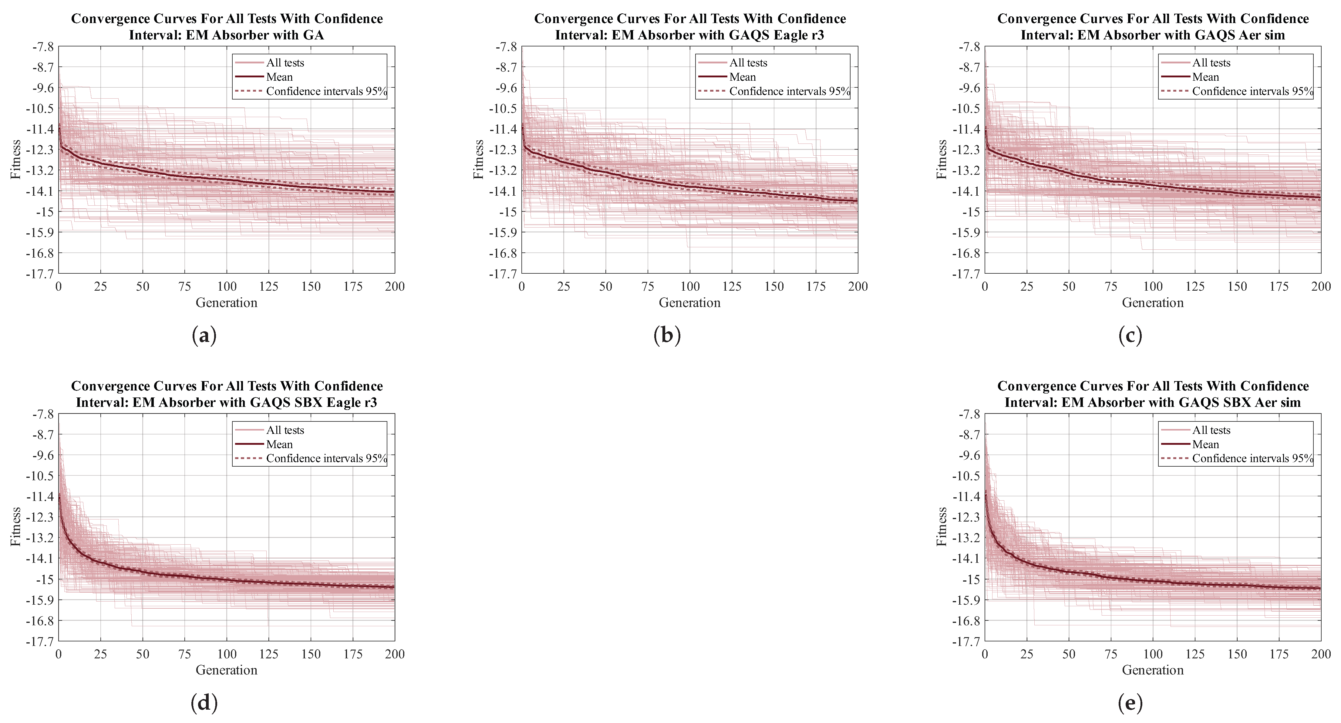
Appendix A
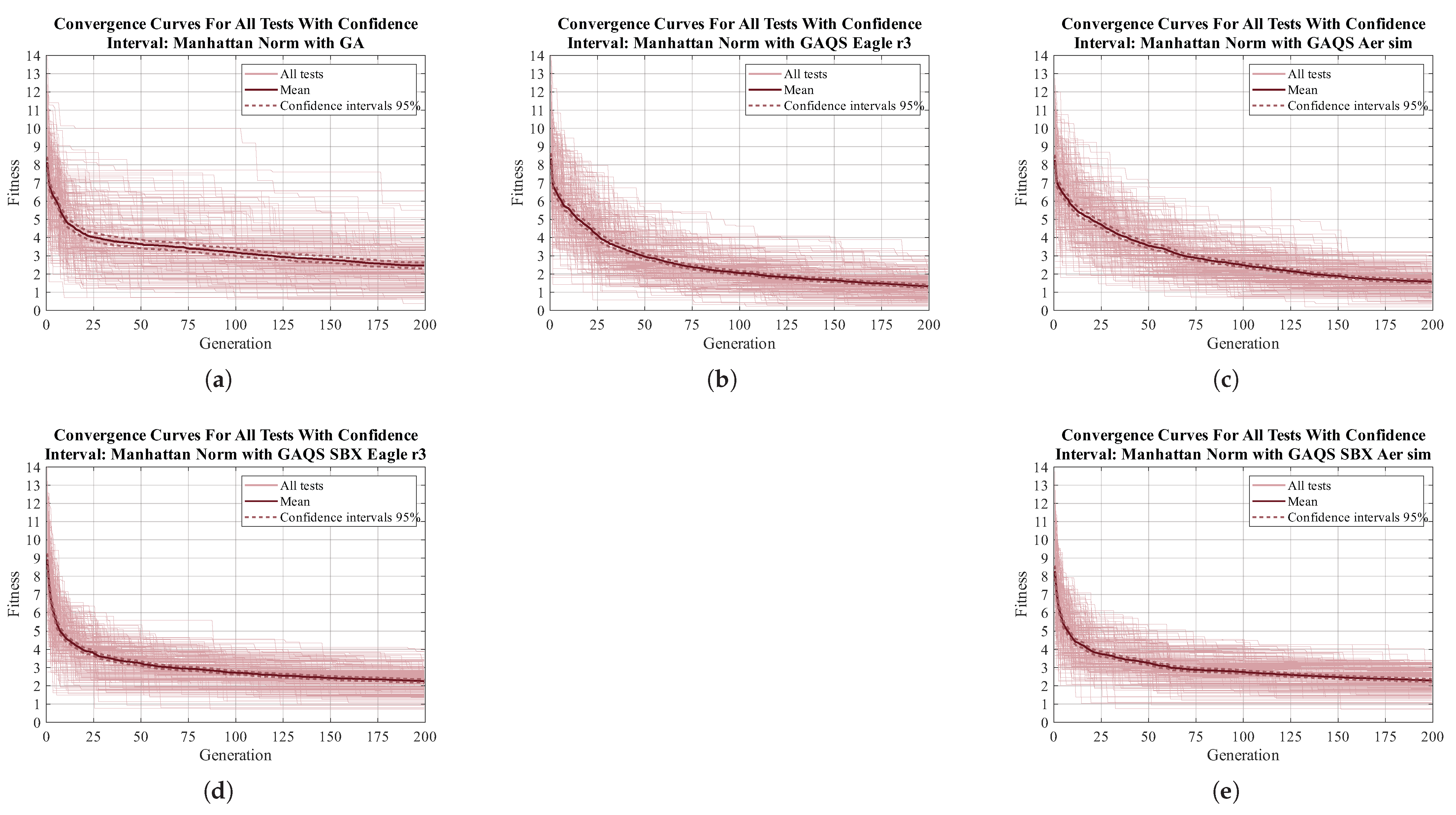
To make the identification of stagnation in the algorithms easier, in this appendix, the convergence curve for each one of the 200 tests done for each algorithm and for each function is presented. The mean and mean’s 95% confidence interval are presented as well. This appendix is divided into five sections, one per function.
Appendix A.1. Manhattan Norm
Figure A1.
Convergence curve for all 200 tests done for Manhattan norm MTF. (a) GA; (b) GAQS Eagle r3; (c) GAQS Aer sim; (d) GAQS SBX Eagle r3; (e) GAQS SBX Aer sim.
Figure A1.
Convergence curve for all 200 tests done for Manhattan norm MTF. (a) GA; (b) GAQS Eagle r3; (c) GAQS Aer sim; (d) GAQS SBX Eagle r3; (e) GAQS SBX Aer sim.
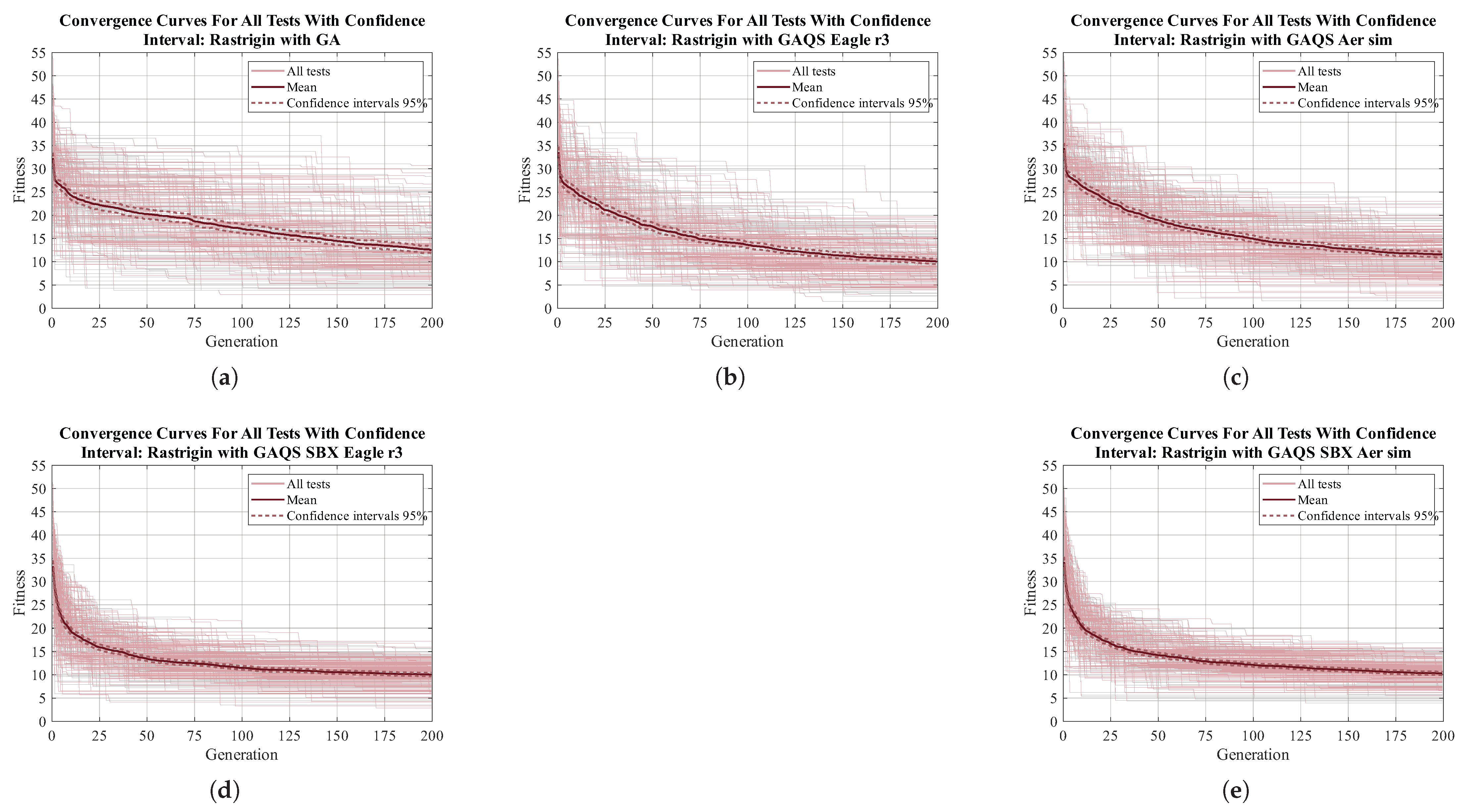
Appendix A.2. Rastrigin Function
Figure A2.
Convergence curve for all 200 tests done for Rastrigin function MTF. (a) GA; (b) GAQS Eagle r3; (c) GAQS Aer sim; (d) GAQS SBX Eagle r3; (e) GAQS SBX Aer sim.
Figure A2.
Convergence curve for all 200 tests done for Rastrigin function MTF. (a) GA; (b) GAQS Eagle r3; (c) GAQS Aer sim; (d) GAQS SBX Eagle r3; (e) GAQS SBX Aer sim.
Appendix A.3. Griewank Function
Figure A3.
Convergence curve for all 200 tests done for Griewank function MTF. (a) GA; (b) GAQS Eagle r3; (c) GAQS Aer sim; (d) GAQS SBX Eagle r3; (e) GAQS SBX Aer sim.
Figure A3.
Convergence curve for all 200 tests done for Griewank function MTF. (a) GA; (b) GAQS Eagle r3; (c) GAQS Aer sim; (d) GAQS SBX Eagle r3; (e) GAQS SBX Aer sim.
Appendix A.4. Microstrip Filter
Figure A4.
Convergence curve for all 200 tests done for microstrip filter EMDP. (a) GA; (b) GAQS Eagle r3; (c) GAQS Aer sim; (d) GAQS SBX Eagle r3; (e) GAQS SBX Aer sim.
Figure A4.
Convergence curve for all 200 tests done for microstrip filter EMDP. (a) GA; (b) GAQS Eagle r3; (c) GAQS Aer sim; (d) GAQS SBX Eagle r3; (e) GAQS SBX Aer sim.
Appendix A.5. EM Absorber
Figure A5.
Convergence curve for all 200 tests done for EM absorber EMDP. (a) GA; (b) GAQS Eagle r3; (c) GAQS Aer sim; (d) GAQS SBX Eagle r3; (e) GAQS SBX Aer sim.
Figure A5.
Convergence curve for all 200 tests done for EM absorber EMDP. (a) GA; (b) GAQS Eagle r3; (c) GAQS Aer sim; (d) GAQS SBX Eagle r3; (e) GAQS SBX Aer sim.
References
- Kangshen, S.; Crossley, J.N.; Lun, A.W.-C. The Nine Chapters on the Mathematical Art: Companion and Commentary; Oxford University Press: Oxford, UK, 1999. [Google Scholar] [CrossRef]
- Burachik, R.S.; Caldwell, B.I.; Kaya, C.Y. A Generalized Multivariable Newton Method. Fixed Point Theory Algorithms Sci. Eng. 2021, 2021, 15. [Google Scholar] [CrossRef]
- Ribeiro, A.A.; Barbosa, J.R.R. Calculus, Constrained Minimization and Lagrange Multipliers: Is the Optimal Critical Point a Local Minimizer? arXiv 2019. [Google Scholar] [CrossRef]
- Lagarias, J.C.; Reeds, J.A.; Wright, M.H.; Wright, P.E. Convergence Properties of the Nelder-Mead Simplex Method in Low Dimensions. SIAM J. Optim. 1998, 9, 112–147. [Google Scholar] [CrossRef]
- Holland, J.H. Adaptation in Natural and Artificial Systems: An Introductory Analysis with Applications to Biology, Control, and Artificial Intelligence; MIT Press: Cambridge, MA, USA, 2010. [Google Scholar] [CrossRef]
- Kennedy, J.; Eberhart, R. Particle Swarm Optimization. In Proceedings of the ICNN’95—International Conference on Neural Networks, Perth, WA, Australia, 1 October 1995; Volume 4, pp. 1942–1948. [Google Scholar] [CrossRef]
- Wolpert, D.H.; Macready, W.G. No Free Lunch Theorems for Optimization. IEEE Trans. Evol. Comput. 1997, 1, 67–82. [Google Scholar] [CrossRef]
- Preskill, J. Quantum Computing in the NISQ Era and Beyond. Quantum 2018, 2, 79. [Google Scholar] [CrossRef]
- Sun, J.; Xu, W.; Feng, B. A global search strategy of quantum-behaved particle swarm optimization. In Proceedings of the IEEE Conference on Cybernetics and Intelligent Systems, Singapore, 1–3 December 2004; pp. 111–116. [Google Scholar] [CrossRef]
- Blekos, K.; Brand, D.; Ceschini, A.; Chou, C.-H.; Li, R.-H.; Pandya, K.; Summer, A. A Review on Quantum Approximate Optimization Algorithm and Its Variants. Phys. Rep. 2024, 1068, 1–66. [Google Scholar] [CrossRef]
- Martinez, G.F.; Zich, R.E. Novel Quantum Computation Based Selection Operator for Genetic Algorithms Applied to Electromagnetic Problems. In Proceedings of the 2024 18th European Conference on Antennas and Propagation (EuCAP), Glasgow, UK, 17–22 March 2024; pp. 1–4. [Google Scholar] [CrossRef]
- Guariso, G.; Sangiorgio, M. Improving the Performance of Multiobjective Genetic Algorithms: An Elitism-Based Approach. Information 2020, 11, 587. [Google Scholar] [CrossRef]
- Nielsen, M.A.; Chuang, I.L. Quantum Computation and Quantum Information: 10th Anniversary Edition, 1st ed.; Cambridge University Press: Cambridge, UK, 2012. [Google Scholar] [CrossRef]
- Martinez, G.F.; Niccolai, A.; Zich, E.L.; Zich, R.E. Quantum Optimization of Microwave Filters. In Proceedings of the 2024 IEEE Joint International Symposium on Electromagnetic Compatibility, Signal & Power Integrity: EMC Japan/Asia-Pacific International Symposium on Electromagnetic Compatibility (EMC Japan/APEMC Okinawa), Okinawa, Japan, 20–24 May 2024; pp. 706–708. [Google Scholar] [CrossRef]
- Martinez, G.; Niccolai, A.; Zich, E.; Zich, R. Accelerated Quantum Selection Optimization of a Microwave Filter. In Proceedings of the 2024 IEEE 1st Latin American Conference on Antennas and Propagation (LACAP), Cartagena de Indias, Colombia, 1–4 December 2024; pp. 1–2. [Google Scholar] [CrossRef]
- Deb, K.; Sindhya, K.; Okabe, T. Self-Adaptive Simulated Binary Crossover for Real-Parameter Optimization. In Proceedings of the 9th Annual Conference on Genetic and Evolutionary Computation, London, UK, 7–11 July 2007; pp. 1187–1194. [Google Scholar] [CrossRef]
- Magnusson, P.; Weisshaar, A.; Tripathi, V.; Alexander, G. Transmission Lines and Wave Propagation, 4th ed.; CRC Press: Boca Raton, FL, USA, 2000. [Google Scholar] [CrossRef]
- Pozar, D.M. Microwave Engineering, 4th ed.; John Wiley & Sons, Inc: Hoboken, NJ, USA, 2012. [Google Scholar]
- Balanis, C.A. Balanis’ Advanced Engineering Electromagnetics, 3rd ed.; John Wiley & Sons: Hoboken, NJ, ISA, 2024. [Google Scholar] [CrossRef]
- Saha, R.K. Coexistence of Cellular and IEEE 802.11 Technologies in Unlicensed Spectrum Bands—A Survey. IEEE Open J. Commun. Soc. 2021, 2, 1996–2028. [Google Scholar] [CrossRef]
- Martinez, G.F.; Niccolai, A.; Zich, R.E. Electromagnetic Multilayer Absorber Design with Quantum Selection Optimization. In Proceedings of the 2025 25th International Conference on the Computation of Electromagnetic Fields (COMPUMAG), Naples, Italy, 22–26 June 2025. [Google Scholar]
Figure 1.
Quantum circuit used for the quantum selection operator (QSO), where the preparation, oracle, Grover diffusion, and measurement stages are presented. The circuit is constructed to implement amplitude amplification, increasing the probability of selecting high-fitness individuals.
Figure 1.
Quantum circuit used for the quantum selection operator (QSO), where the preparation, oracle, Grover diffusion, and measurement stages are presented. The circuit is constructed to implement amplitude amplification, increasing the probability of selecting high-fitness individuals.
Figure 2.
The considered mathematical test functions are plotted in two dimensions: (a) Manhattan norm, (b) Rastrigin function, and (c) Griewank function. These functions are used to assess the exploration and convergence behavior of the algorithms.
Figure 2.
The considered mathematical test functions are plotted in two dimensions: (a) Manhattan norm, (b) Rastrigin function, and (c) Griewank function. These functions are used to assess the exploration and convergence behavior of the algorithms.
Figure 3.
The schematic of the microstrip filter used as an electromagnetic design problem is shown. The filter is constructed using symmetric transmission lines, with widths representing the optimization variables.
Figure 3.
The schematic of the microstrip filter used as an electromagnetic design problem is shown. The filter is constructed using symmetric transmission lines, with widths representing the optimization variables.
Figure 4.
A schematic representation of the multilayer electromagnetic absorber is presented. Each layer is modeled as a lossy dielectric slab contributing to power dissipation and reflection reduction.
Figure 4.
A schematic representation of the multilayer electromagnetic absorber is presented. Each layer is modeled as a lossy dielectric slab contributing to power dissipation and reflection reduction.
Figure 5.
Evolution of the mean fitness value across 200 tests for each algorithm, using both quantum circuit measurement techniques. The following benchmark problems are presented: (
a) Manhattan norm, (
b) Rastrigin function, (
c) Griewank function, (
d) Microstrip filter, and (
e) electromagnetic absorber. The shaded backgrounds denote convergence phases defined as EGs (early generations), MGs (middle generations), and LGs (late generations) for mathematical functions, and IGs (initial generations) and FGs (final generations) for electromagnetic design problems. Lower fitness values are preferable. All individual optimization runs and the confidence interval of the means are available in
Appendix A.
Figure 6.
Convergence speed of the mean fitness value for all 200 tests performed per algorithm, using both quantum circuit measurement techniques. The benchmarks include (a) Manhattan norm, (b) Rastrigin function, (c) Griewank function, (d) Microstrip filter, and (e) electromagnetic absorber. Displayed curves include both the instantaneous square root of the rate of fitness change and a 10-sample moving average. Colored backgrounds correspond to convergence phases: EGs (early generations), MGs (middle generations), and LGs (late generations) for mathematical functions, and IGs (initial generations) and FGs (final generations) for design problems. Higher values indicate faster convergence.
Figure 7.
Box plots of the final fitness values obtained across 200 runs for each algorithm and quantum measurement method are shown for (a) Manhattan norm, (b) Rastrigin function, (c) Griewank function, (d) Microstrip filter, and (e) electromagnetic absorber. Lower medians, smaller interquartile ranges (IQRs), and fewer high-fitness outliers indicate more consistent and effective optimization.
Figure 8.
The average execution time per generation is presented for each algorithm across all benchmark problems. Measurements were taken on a standard laptop. Bars are grouped by test function: Manhattan norm, Rastrigin, Griewank, Microstrip filter, and electromagnetic absorber. Increased computation time observed in GAQS SBX is primarily due to the more complex crossover and mutation operations.
Table 1.
Considered mathematical test functions.
Table 1.
Considered mathematical test functions.
| Function | Equation | Bounds | Type |
|---|
| Manhattan norm | | | Convex |
| Rastrigin function | | | Non-convex |
| Griewank function | | | Non-convex |
Table 2.
Parameters used in the optimization algorithms.
Table 2.
Parameters used in the optimization algorithms.
| Parameter | GA | GAQS | GAQS SBX |
|---|
| Population size | 32 | 32 | 32 |
| Mutation rate | | | |
| Number of qubits | | 6 | 6 |
| | 3 | 3 |
| | | 0.5 |
| | | 0.5 |
Table 3.
Dielectric characteristics of the materials used for the multilayer electromagnetic absorber.
Table 3.
Dielectric characteristics of the materials used for the multilayer electromagnetic absorber.
| Material Name | Relative Electric Permittivity () | Loss Tangent |
|---|
| | 0.050 |
| | 0.100 |
| | 0.057 |
| | 0.060 |
Table 4.
p-values obtained from the Wilcoxon signed-rank test performed on the final results. confirms the hypothesis in the header .
Table 4.
p-values obtained from the Wilcoxon signed-rank test performed on the final results. confirms the hypothesis in the header .
| | GAQS Outperforms GA | GAQS SBX
Outperforms GA | Aer Simulator Outperforms Eagle r3 |
|---|
| | In GAQS | In GAQS SBX |
| Manhattan norm | 0.000 | 0.000 | 0.000 | 0.208 |
| Rastrigin | 0.000 | 0.000 | 0.000 | 0.130 |
| Griewank | 0.000 | 0.000 | 0.000 | 0.350 |
| Microstrip Filter | 0.000 | 0.000 | 0.053 | 0.034 |
| EM Absorber | 0.000 | 0.000 | 0.044 | 0.830 |
| Disclaimer/Publisher’s Note: The statements, opinions and data contained in all publications are solely those of the individual author(s) and contributor(s) and not of MDPI and/or the editor(s). MDPI and/or the editor(s) disclaim responsibility for any injury to people or property resulting from any ideas, methods, instructions or products referred to in the content. |
© 2025 by the authors. Licensee MDPI, Basel, Switzerland. This article is an open access article distributed under the terms and conditions of the Creative Commons Attribution (CC BY) license (https://creativecommons.org/licenses/by/4.0/).


