Classification of Complex Power Quality Disturbances Based on Lissajous Trajectory and Lightweight DenseNet

Abstract

With the increase in the penetration rate of distributed sources and loads, the sensor monitoring data is increasing dramatically. Power grid maintenance services require a rapid response in power quality data analysis. To achieve a rapid response and highly accurate classification of power quality disturbances (PQDs), this paper proposes an efficient classification algorithm for PQDs based on Lissajous trajectory (LT) and a lightweight DenseNet, which utilizes the concept of Lissajous curves to construct an ideal reference signal and combines it with the original PQD signal to synthesize a feature trajectory with a distinctive shape. Meanwhile, to enhance the ability and efficiency of capturing trajectory features, a lightweight L-DenseNet skeleton model is designed, and its feature extraction capability is further improved by integrating an attention mechanism with L-DenseNet. Finally, the LT image is input into the fusion model for training, and PQD classification is achieved using the optimally trained model. The experimental results demonstrate that, compared with current mainstream PQD classification methods, the proposed algorithm not only achieves superior disturbance classification accuracy and noise robustness but also significantly improves response speed in PQD classification tasks through its concise visualization conversion process and lightweight model design.

1. Introduction

1.1. Background and Motivation

With the development of smart grid technology and the proposal of decarbonization goals, the proportion of distributed sources and loads, mainly new energy, connected to the grid has been continuously increasing, bringing abundant social benefits and various accompanying challenges [1]. In particular, the massive influx of power electronic devices has led to a surge in monitoring data for power system health situational awareness (PSA), which is centered on power quality (PQ) monitoring. Meanwhile, due to the unpredictable changes in renewable energy sources, external environments, and actual working conditions, PQ issues are becoming more complex [2]. According to existing reports, PQ issues are estimated to cause annual economic losses amounting to several billion dollars worldwide [3,4]. In addition to the financial impact, they adversely affect industrial operations, commercial activities, and residential life, and may even pose threats to critical public infrastructure, such as hospitals and transportation systems. Equipment damage increases maintenance costs and prolongs recovery time, while large-scale power outages can lead to social disorder and result in immeasurable indirect losses [5], thereby drawing significant attention and concern toward PSA.

The premise of effective PSA is to accurately and rapidly identify the types of power quality disturbances (PQDs) in monitoring data. The results of PQD classification can guide power grid companies in formulating targeted maintenance decisions and implementing precise maintenance to ensure the safe and stable operation of the power grid while reducing operation and maintenance costs. In modern smart grids, the increasing penetration of distributed sources and power electronic devices has significantly intensified the coupling and complexity of PQDs. In extreme cases, up to four different single-disturbance types may be superimposed on a single waveform, which presents additional challenges in overcoming abnormal changes in voltage waveforms. Furthermore, with the massive growth of monitoring data from PQ sensors, grid operation and maintenance departments have established higher demands for the efficiency of PQD situation awareness. Consequently, there is an urgent need to develop PQD classification algorithms that offer both high efficiency and high accuracy to meet the requirements of modern power systems for real-time and intelligent operation and maintenance.

1.2. Literature Review

Traditional PQD classification methods mainly rely on the manual analysis of abnormal monitoring waveform data collected by sensors and judging the specific type of event based on empirical knowledge. However, this method is time-consuming and costly, and it can no longer meet the practical needs for analysis efficiency and safety in the era of data surge. To address the time-consuming nature and subjectivity of manual analysis, there has been a growing exploration of automated signal feature extraction and recognition technologies for PQD classification tasks, aiming to reduce reliance on human expert knowledge. Profiting from the development of computer technology and advanced metering infrastructure (AMI) with high recording frequency, data-driven PQD identification methods have emerged. Due to their efficient processing flow and excellent identification effect, they have replaced the traditional expert experience-based manual judgment method and have become the mainstream direction in current PQD identification research and application. They can be roughly divided into machine learning-based identification and deep learning-based identification.

Machine learning-based identification algorithms usually combine manual feature extraction methods with machine learning classifiers to achieve event identification, such as wavelet transform (WT) with a support vector machine (SVM) [6], Stockwell transform (ST) with random forest (RF) [7], and variation mode decomposition (VMD) with Light GBM (LGBM) [8]. These methods have all achieved accurate identification of PQDs to a certain extent. However, the parameter selection and processing involved in manual feature extraction methods are cumbersome, and they rely heavily on experts’ knowledge of PQDs. Considering the interactive coupling of disturbances caused by the large-scale integration of power electronic devices, this reliance limits their generalization to complex PQDs, making it difficult to meet the classification requirements of PQDs in the context of the new power system.

To improve the generalization performance of algorithms, deep learning methods are widely introduced into PQD identification. Depending on the form of data input into the model, there are mainly two mainstream research directions: one is to use the collected sequence data directly as input for event classification. By combining a full convolutional network (FCN) with a long short-term memory network (LSTM), Ref. [9] proposed a PQD identification method with strong anti-noise and anti-interference capabilities. Considering the characteristics of PQDs, Ref. [10] designed a deep convolutional neural network (CNN) that can automatically extract multi-scale features from a large number of event samples and then complete PQD identification. However, due to the sequential nature of time series embedding, which has many important characteristics, these characteristics lie outside the scope of a typical time domain analysis. Therefore, the sequence classification method struggles to fully mine the PQD signal features and often performs poorly in multi-class coupling disturbance classification. The second method involves converting the sequence data into image data through visualization methods, wich serve as the input for mainstream image recognition models to identify event types. In [11], the gram angular field (GAF) is used to convert the 1D sequence data into 2D images with different texture features, which are then used as the input for the CNN in PQD identification. However, the GAF coding process loses important original sequence information, such as amplitude. To address the abovementioned issues, Ref. [12] proposes a trajectory circle (TC)-based sequence visualization method that captures the envelope trajectory of the original signal through the Hilbert transform (HT) and combines it with the ResNet18 model to achieve the identification of PQD types. However, when HT is performed on the sampled signal, most PQDs lead to curve jumping and endpoint effects, which distort the analytical signal, affect the characteristics of the TC, and reduce classification accuracy. To address this issue, Ref. [13] improved the TC visualization method using the extended sliding window mean value algorithm (ESM) and obtained the improved TC (ITC) feature image corresponding to PQDs. Combined with the large-scale image recognition network ResNet50, it achieved high-precision PQD classification results. However, the calculation of ESM when dealing with curve jumping and endpoint effects is extremely cumbersome, which greatly affects data conversion efficiency. Moreover, when dealing with complex PQD signals, it is prone to causing envelope trajectory feature loss.

1.3. Research Objectives and Contributions

After a thorough analysis, it can be said that deep learning methods have emerged as the mainstream techniques in the PQD classification field due to their capability for automatic feature extraction and strong generalization performance. Meanwhile, classification algorithms that integrate signal visualization conversion methods with advanced image recognition networks, leveraging their ability to deeply mine and capture features from temporal sequence signals, have become a highly promising solution. However, existing studies on complex PQD classification using signal visualization technology combined with image recognition networks are limited and primarily focus on improving accuracy performance while overlooking the efficiency performance of sequence visualization methods and deep learning classifiers in PQD classification tasks. However, when developing classification algorithms, a key point that requires special attention is the efficient calculation and analysis of the designed scheme, which is particularly crucial for addressing the analysis and response challenges brought about by the massive PQ monitoring data in modern power systems. Moreover, in contrast, less effort has been made to classify complex PQDs. In modern power systems, it is possible for up to four distinct single disturbances to be superimposed and intertwined on the same waveform, e.g., identifying a voltage sag combined with harmonic, oscillatory transient, and flicker on the same waveform. To address the abovemetioned issues, this paper proposes an efficient PQD classification framework based on Lissajous trajectory (LT) and lightweight DenseNet, designed to fully meet the analysis demands of power grid operation and maintenance departments for massive and complex PQ monitoring data in the new power system. The main contributions of this paper are summarized as follows:

(1)

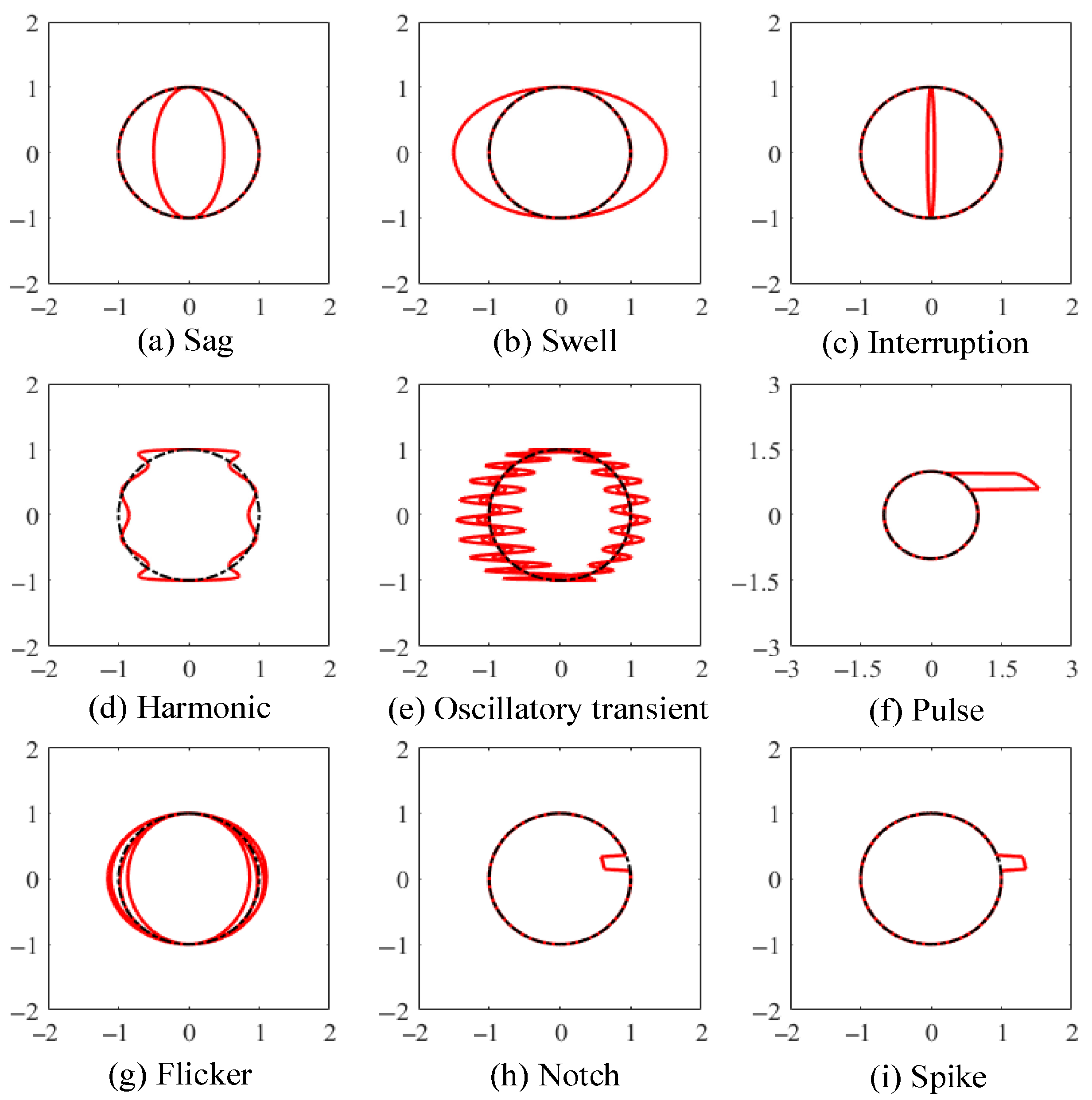
A rapid one-dimensional sequence visualization method is proposed, which is built upon the new concept of LT. Once a disturbance occurs, the shape of LT will change significantly according to the disturbance type, generating a clear and distinguishable characteristic trajectory. Meanwhile, the LT synthesis process is very concise. It only requires the construction of a simple ideal reference signal to be completed, which can meet the real-time data conversion requirements in the context of a sharp increase in monitoring data.

(2)

Leveraging the dense connectivity feature extraction mechanism of DenseNet, a lightweight image recognition network (L-DenseNet) with both classification accuracy and streamlined architecture is developed as the skeleton model for the PQD classification task. This model includes two primary modules: the dense connected learning module and the classification module. To further enhance the model’s deep feature extraction capability, the convolutional block attention module (CBAM) is introduced between the two modules of L-DenseNet to enhance its ability to focus on and capture fine-grained feature information. By integrating L-DenseNet with the CBAM module, high-precision PQD classification performance is achieved while significantly reducing the model’s parameter count and computational complexity.

(3)

The integrated classification framework combining LT and lightweight L-DenseNet-CBAM can effectively extract nonlinear fluctuation feature information from complex PQD signals, enhancing classification accuracy under both noise-free and noisy conditions while significantly reducing computation time. Extensive experiments are conducted based on the simulation dataset generated according to the IEEE std1159 and real-world measured data monitored by the power grid substation to evaluate the performance of the proposed algorithm against several state-of-the-art classification techniques. Compared with the eight existing mainstream PQD classification methods, the proposed algorithm achieves the best comprehensive performance in terms of classification accuracy and efficiency.

2. PQD Signal Visualization Processing Based on Lissajous Trajectory

2.1. Model Construction of PQDs

The generation of PQDs often accompanies abnormal faults in system equipment and interference from external factors. If they cannot be detected and identified in a timely and accurate manner, it will be impossible to complete the repair of abnormal states the first time, which poses serious safety risks and economic losses to the power grid. The modeling method for PQDs can be obtained according to IEEE Std 1159-2019 [14]. Its representative equations are shown in

Table 1. Mathematical models of PQDs.

Label	Type of PQDs	Mathematical Model	Parameters
C0	Normal	$f\left(t\right)=\sin \left(\omega t\right)$	$\omega =2\pi f_0,f_0=50\mathrm{Hz}$
C1	Sag	$f\left(t\right)=\{1-\alpha [\epsilon (t-t_1)-\epsilon (t-t_2)\left]\right\}\sin \left(\omega t\right)$	$0.1\le \alpha \le 0.9,T\le t_2-t_1\le 9T$
C2	Swell	$f\left(t\right)=\{1+\alpha [\epsilon (t-t_1)-\epsilon (t-t_2)\left]\right\}\sin \left(\omega t\right)$	$0.1\le \alpha \le 0.8,T\le t_2-t_1\le 9T$
C3	Interruption	$f\left(t\right)=\{1-\alpha [\epsilon (t-t_1)-\epsilon (t-t_2)\left]\right\}\sin \left(\omega t\right)$	$0.9\le \alpha \le 1,T\le t_2-t_1\le 9T$
C4	Harmonic	$f(t)=\sin \left(\omega t\right)+{\displaystyle \sum _{i=\mathrm{3,5},7}}{\alpha }_i\sin \left(i\omega t\right)$	$0.05\le {\alpha }_i\le 0.15$
C5	Oscillatory transient	$f\left(t\right)=\sin \left(\omega t\right)+\alpha e^{-(t-t_1)/\tau }\sin \left(\beta \omega t\right)\cdot \left[\epsilon \right(t-t_1)-\epsilon (t-t_2\left)\right]$	$0.1\le \alpha \le 0.8,0.5\mathrm{T}\le t_2-t_1\le 3T$ $0.008\le \tau \le 0.04,8\le \beta \le 32$
C6	Pulse	$f\left(t\right)=\sin \left(\omega t\right)+\alpha \left[\epsilon \right(t-t_1)-\epsilon (t-t_2\left)\right]$	$1\le \alpha \le 3,1\mathrm{ms}\le t_2-t_1\le 3\mathrm{ms}$
C7	Flicker	$f\left(t\right)=\left[1+\alpha \sin \left(\beta \omega t\right)\right]\sin \left(\omega t\right)$	$0.1\le \alpha \le 0.2,0.1\le \beta \le 0.5$
C8	Notch	$f(t)=\sin \left(\omega t\right)-\mathrm{sgn}(\sin \left(\omega t\right))\times \{{\displaystyle \sum _{n=0}^9}k\times [\epsilon (t-(t_1+0.02n))-\epsilon (t-(t_2+0.02n))]\}$	$0.1\le k\le 0.4,0\le t_2,t_1\le 0.5T$ $0.01T\le t_2-t_1\le 0.05T$
C9	Spike	$f(t)=\sin \left(\omega t\right)+\mathrm{sgn}(\sin \left(\omega t\right))\times \{{\displaystyle \sum _{n=0}^9}k\times [\epsilon (t-(t_1+0.02n))-\epsilon (t-(t_2+0.02n))]\}$	$0.1\le k\le 0.4,0\le t_2,t_1\le 0.5T$ $0.01T\le t_2-t_1\le 0.05T$

. Among them, the nine types of PQDs are all single disturbances, represented by C1–C9, and the normal signal is represented by C0. The waveform diagrams of C0-C9 are shown in Figure 1.

Complex PQDs are usually composed of multiple single PQDs, which contain various categories and different start and end times. The resulting composite waveforms are more complex and variable, with stronger randomness. This presents challenges for the generalization of traditional identification algorithms. The complex PQDs can be expressed as follows:

$$f\left(t)=\lambda \right(t\left)\sin \right(\omega t)+\phi \left(t\right)$$

(1)

where ω is the nominal system frequency, and λ(t) represents the multiplication coefficient module of the PQD signal, including sag, swell, interruption, and flicker. φ(t) represents the superposition module of PQD signal, including harmonic, oscillatory transient, pulse, notch, and spike.

2.2. Sequence Visualization via Lissajous Trajectory

In mathematics, Lissajous curves refer to the trajectories of a family of curves synthesized by two sinusoidal vibrations in mutually perpendicular directions. Due to their diversity in image generation, this concept is often applied in the field of signal and image processing [15]. In recent years, the application scope of Lissajous curves has gradually expanded in power system engineering, such as for identifying fault locations in transmission lines [16] or monitoring the health status of power systems [17]. However, the two synthesis components selected in the construction of Lissajous curves in existing studies are both voltage waveforms and current waveforms, which are not applicable to the PQD classification issue targeted in this paper. This is because the research object of this topic only targets the single physical quantity of voltage and its single-phase data. To the best of our knowledge, no prior study has applied Lissajous synthesis technology to PQD classification research.

To fully extract the sequence feature information of single-phase voltage signals, this paper proposes a new Lissajous curve concept called the Lissajous trajectory. This concept is motivated by the observation that the LT not only offers comprehensive and precise temporal sequence feature extraction capabilities for PQD signals but also has rapid visualization conversion efficiency. The LT is constructed by synchronously synthesizing curves at each time point, using an ideal reference signal and the target disturbance signal as the vertical and horizontal coordinates in a Cartesian coordinate system, respectively, resulting in the LT representation corresponding to the target PQD signal. When no disturbance occurs, the LT corresponding to a normal signal forms a standard circular trajectory. Once a disturbance occurs, the shape of the corresponding LT of the voltage signal will change, and the specific shape after the change will depend on the type of PQDs. Specifically, an ideal reference signal, U_ISP, with an amplitude of 1 and a phase different from the target signal, is constructed, which differs from the target signal by a phase, φ, where φ is set to 90° (the lead or lag of phase angle only change the direction of the trajectory features and have no impact on the final result). The expression of U_ISP is as follows:

$$U\mathrm{ISP}=\sin (\omega t+{\displaystyle \frac{\pi }{2}})$$

(2)

Based on the concept of LT curve synthesis, the waveform of the PQD signal defined in (1) and the ideal reference waveform in (2) are assigned as the horizontal and vertical coordinates, respectively, in a Cartesian coordinate system to generate LT characteristic curves corresponding to various PQD signals. To demonstrate the synthesis effect of LT on PQDs, nine of the most representative single disturbance signals given in IEEE Std 1159 (Table 1) are used for illustration. To align with the actual operating and measurement conditions of the power grid, the fundamental frequency is set to 50 Hz, and the sampling frequency is set to 12.8 kHz. The disturbance signals are sliced every four cycles to generate the Lissajous characteristic trajectories of nine single-PQD signals, as shown in Figure 2a–i. It can be seen in Figure 2 that the characteristic trajectories corresponding to various disturbances are clear and easily distinguishable. This not only facilitates feature extraction after the composite superposition of disturbances but also lays the foundation for accurate PQD classification using deep learning networks. Furthermore, compared to existing signal visualization methods such as GAF [11], TC [12], and ITC [13], the conversion process of LT is remarkably concise and efficient, requiring only the construction of an ideal reference signal for the synthesis of the horizontal and vertical coordinates.

3. PQD Classification Model Based on Lightweight DenseNet

3.1. Fundamental Principles of DenseNet

As a classic deep learning classification network architecture with outstanding performance in existing image classification tasks [18], DenseNet achieves feature reuse by leveraging its unique dense connection mechanism. This mechanism enhances the transmission and reuse capabilities of feature maps, thereby allowing the network to more comprehensively and fully capture critical local detail features within images. In addition, DenseNet significantly reduces redundant parameters and lowers model complexity through feature reuse. This compact structure not only enhances training efficiency but also effectively alleviates overfitting problems when the sample size is limited or the categories are unbalanced. Therefore, this paper adopts DenseNet as the foundational architecture for the PQD classification model.

DenseNet primarily consists of transition layers and dense blocks (DB). The transition layer includes convolutional and pooling layers, primarily functioning to reduce the size of feature maps. The DB introduces a novel connectivity mechanism, where the output of all preceding layers serves as the input for the current layer, and its output subsequently becomes the input for all following layers. In contrast to the residual block of ResNet, which consists of two convolutional layers and cross-layer connections, the DB of DenseNet further incorporates inter-layer connections in addition to cross-layer links. These additional inter-layer connections facilitate the repeated utilization of input features, ensuring maximum information flow. The structure of the DB is illustrated in Figure 3. In this architecture, global and essential feature information can be more comprehensively extracted, leading to more accurate and efficient training outcomes.

3.2. Design of Lightweight DenseNet Architecture

To balance classification accuracy and efficiency, this paper develops a more streamlined and lightweight DenseNet architecture, named L-DenseNet, as the backbone network for the PQD classification model while ensuring classification accuracy. The network structure is shown in

Table 2. Network structure of the lightweight L-DenseNet model.

Layer	Module Composition (Growth Rate k = 32)	Output Dimensions
Convolutional	7 × 7 Conv, stride = 2	64 × 64 × 64
Pooling	3 × 3 Max pooling, stride = 2	32 × 32 × 64
DB1	$[\begin{array}{c}1\times 1\mathrm{Conv}\\ 3\times 3\mathrm{Conv}\end{array}]\times 3$	32 × 32 × 160
Transition	1 × 1 Conv	16 × 16 × 80
	2 × 2 Average pooling, stride = 2
DB2	$[\begin{array}{c}1\times 1\mathrm{Conv}\\ 3\times 3\mathrm{Conv}\end{array}]\times 8$	16 × 16 × 336
Transition	1 × 1 Conv	8 × 8 × 168
	2 × 2 Average pooling, stride = 2
DB3	$[\begin{array}{c}1\times 1\mathrm{Conv}\\ 3\times 3\mathrm{Conv}\end{array}]\times 12$	8 × 8 × 552
Classification	Adaptive average pooling	1 × 1 × 552
	Fully connected, Softmax	1 × 1 × 41

. L-DenseNet consists of three DBs, each composed of 3, 8, and 12 stacked convolutional layers, with a growth rate of k = 32. To enhance computational efficiency and network compactness, bottleneck layers and transition layers are introduced to achieve dimensional reduction of feature maps. The bottleneck layer is embedded within the DB and consists of a 1 × 1 convolutional layer, a batch normalization (BN) layer, and an activation layer (ReLU). The transition layer is primarily composed of a BN layer, a 1 × 1 convolutional layer, and a 2 × 2 average pooling layer. Its position is set between two DBs and is used to further compress the size of the feature map. To balance information retention and parameter overhead, the compression coefficient of the transition layer is set to 0.5.

3.3. Attention Mechanism

The convolution and pooling operations of CNNs assume equal importance for each channel in the feature map by default. However, since the significance of the information carried by each channel varies, treating all channels as equally important lacks rationality. The CBAM convolutional block attention mechanism is an attention module designed to enhance the CNN’s feature capture capability, as proposed by Woo et al. [19]. The primary objective of this module is to improve the model’s ability to perceive crucial feature information by incorporating channel attention and spatial attention, thereby enhancing classification performance without increasing network complexity. Consequently, this paper introduces the CBAM attention mechanism to strengthen the network’s focus on detailed features within various LT of PQDs, enabling it to achieve better classification results.

The CBAM attention mechanism module is mainly composed of two sub-modules: the channel attention module (CAM) and the spatial attention module (SAM). Its specific structure is shown in Figure 4. The main basis for CAM to allocate the weight coefficients is the importance of the feature channels. Firstly, global average pooling and max pooling are applied to aggregate information across all channels, generating two distinct one-dimensional feature vectors. These vectors are then processed through fully connected layers, followed by element-wise addition and an activation function to compute the channel attention weight M_CAM, which is calculated as follows:

$$M_{\mathrm{CAM}}(F)=\mathrm{sigmoid}(\mathrm{MLP}(\mathrm{AvgPool}(F))+\mathrm{MLP}(\mathrm{MaxPool}(F)))$$

(3)

where MLP represents the computation performed by fully connected layers. AvgPool and MaxPool represent average pooling and max pooling operations, respectively. F refers to the input feature map of the CAM module. After M_CAM is obtained, it is element-wise multiplied with F to produce the feature map F₁, which is weighted by CAM.

After the feature map, F₁, which is processed by CAM weighting, is obtained, it is used as input for the SAM module to further capture important spatial regions. Max pooling and average pooling are spatially applied to F₁, generating two two-dimensional feature maps, which are then concatenated and processed through a convolution operation and activation function to ultimately produce the spatial attention weight M_SAM. This weight is then applied to obtain the feature map weighted by SAM. The formula for computing the spatial attention weight is as follows:

$$M_{\mathrm{SAM}}(F)=\sigma (f^{3\times 3}([\mathrm{AvgPool}(F);\mathrm{MaxPool}(F)]))=\sigma (f^{3\times 3}([F_{\mathrm{avg}}^S;F_{\max }^S]))$$

(4)

where f^3×3 represents a 3 × 3 convolution operation used for dimensional reduction.

3.4. Overall Framework Construction for PQD Classification

Leveraging the imaging advantages of the LT-based visualization method and the high training efficiency and strong deep feature extraction capability of the L-DenseNet-CBAM fusion model, this paper proposes a novel PQD classification algorithm based on LT and lightweight DenseNet. The overall classification framework is illustrated in Figure 5 and consists of four main components: the signal visualization module, the dense connected learning module, the attention mechanism module, and the classification module.

(1)

Signal visualization module: Firstly, the ideal reference signal UISP is constructed using (1). The values of the UISP and the PQD temporal sequence sampling signal at the same time point serve as the horizontal and vertical coordinates in a Cartesian coordinate system, respectively, for curve synthesis, thereby generating the LT representation corresponding to the target PQD signal. Then, the synthesized LT is mapped onto a fixed-size image space and normalized using a unified coordinate range to generate a two-dimensional image with a resolution of 128 × 128 pixels and three RGB channels. This method indirectly enhances the classification accuracy of PQDs at the data representation level by generating two-dimensional trajectory images with clear and distinguishable features.

(2)

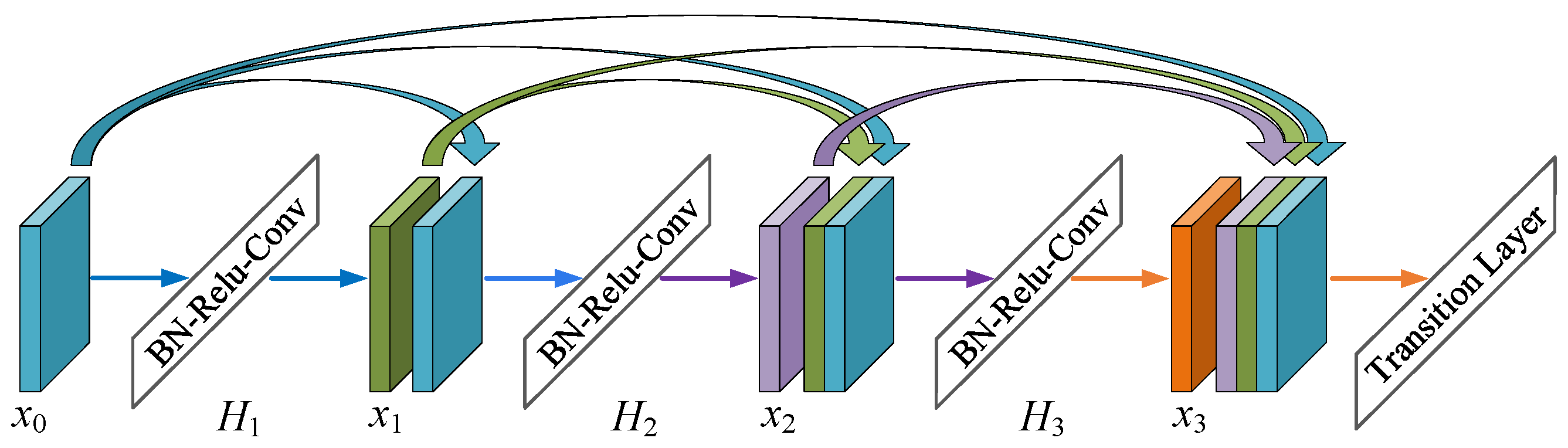
Dense connected learning module: This module comprises DBs and transition layers. RGB feature maps undergo convolution and dimension reduction via $7\times 7$ convolution layers and $3\times 3$ max-pooling layers to extract shallow feature information. Following feature extraction, the feature information needs to traverse three sets of DBs, with a transition layer connecting every two sets of DBs. When passing through DBs, feature reuse is performed on feature maps from different layers in the channel dimension based on a dense connection mechanism, which is conducive to the extraction of deeper feature information and the combination of shallow- and deep-layer information in the network, which greatly improves feature utilization. Meanwhile, transition layers are introduced to reduce feature dimensions, which reduces network parameter redundancy and enhances the overall efficiency of the model’s learning and computation.

(3)

Attention mechanism module: Adding the CBAM attention module between the dense connection learning module and the classification module of DenseNet-S can effectively enhance the network’s recognition precision, as evidenced by extensive experimentation. The feature map, $F$, output by Dense Block 3 enters the CAM module, where max-pooling and average-pooling operations are performed, resulting in two $1\times 1\times 552$ one-dimensional feature vectors. Then, the two feature vectors are sent into the full connection layer for calculation and the sum operation. After the activation operation, the CAM module generates channel attention weights, $M_{\mathrm{C}\mathrm{A}\mathrm{M}}$, which are then multiplied with the feature map, $F$, to derive $F_1$, which is the input feature map for the SAM module. In the SAM module, the feature map, $F_1$, undergoes separate max-pooling and average-pooling operations according to spatial position, and the two results are spliced to generate an $8\times 8\times 2$ feature map. Subsequently, this map undergoes dimensional reduction through a 1-channel convolution layer. The spatial attention weight, $M_{\mathrm{S}\mathrm{A}\mathrm{M}}$, is then obtained via Sigmoid function activation. Ultimately, the feature obtained by multiplying the weights, $M_{\mathrm{S}\mathrm{A}\mathrm{M}}$, with the input feature map, $F_1$, represents the feature enhanced by CBAM.

(4)

Classification module: This module consists of an adaptive average-pooling layer, two fully connected layers, and a Softmax classifier. Firstly, the feature maps enhanced by CBAM are converted into one-dimensional feature vectors using adaptive average pooling, which are then input into the fully connected layer. Then, the feature information output from the fully connected layer is input into the Softmax classifier. The Softmax function is used to calculate the probability value of each PQD type corresponding to the LT feature image, and the category with the maximum value is output as the classification result to achieve the identification of the PQD type.

Figure 5. PQD classification framework based on LT and lightweight DenseNet. The red lines represent the LT corresponding to PQDs with waveform distortion, while the dotted lines indicate the LT corresponding to normal signal waveforms.

Figure 5. PQD classification framework based on LT and lightweight DenseNet. The red lines represent the LT corresponding to PQDs with waveform distortion, while the dotted lines indicate the LT corresponding to normal signal waveforms.

4. Case Studies: Part I: Simulation Analysis

4.1. Experimental Environment and Data Preparation

In modern power systems, the widespread integration of distributed sources and loads, as well as power electronic devices, has exacerbated the composite nature of PQDs. To more comprehensively cover the analysis scope of complex PQDs under real-world power grid operating conditions, according to IEEE Standard 1159-2019, a total of 31 types of composite disturbances are generated by superimposing nine basic disturbance mathematical models. Among these, the numbers of double, triple, and quadruple disturbances are 16, 10, and 5, respectively. The configuration parameters for the amplitude variation, duration, and other features of the one-dimensional PQD signal waveforms are shown in Table 1. The nominal system frequency is 50 Hz, with a sampling rate of 12.8 kHz, and each sampling process covers four cycles. For each disturbance type, 1000 samples with uniformly distributed amplitude and phase are generated under different signal-to-noise ratio (SNR) conditions (no noise, 60 dB, 40 dB, and 20 dB), ensuring coverage of most disturbance scenarios. Through the PQD data visualization process in Section 2.2, the samples are converted into two-dimensional feature trajectory images using Lissajous curves, resulting in a total of 41 types of the PQD LT dataset.

This study constructs the PQD classification model based on the PyTorch 1.12.1 deep learning framework, with detailed experimental environment parameters as shown in

Table 3. Parameters of the experimental environment.

Configuration	Parameter	Configuration	Parameter
OS	Win10 64bit	Python	3.9
CPU	Ryzen 3970X	Pyts	0.12.0
GPU	RTX 3090	Pytorch	1.12.1
RAM	DDR4 128G	CUDA	11.6

. The LT dataset is divided into training, validation, and testing sets in a ratio of 60%, 20%, and 20%, respectively. During model training, we use the cross-validation method to obtain the optimal deep learning classifier based on classification accuracy and loss performance on the validation set.

4.2. Hyperparameter Settings and Performance Evaluation Metrics

To optimize the overall performance of the classification algorithm, hyperparameter tuning is required for the deep learning model. This tuning process is carried out by observing the performance metrics on the validation and test sets. Regarding the hyperparameter settings, the initial learning rate is set to 0.0001, the number of training epochs is 50, and the batch size is 64. The training process adopts the cross-entropy loss function for loss computation and employs the Adam optimizer to update the model parameters.

To comprehensively evaluate the overall performance of the proposed algorithm in PQD classification tasks, in terms of the accuracy metric, we adopt the average classification accuracy (Acc) for performance evaluation. In terms of the efficiency metric, we adopt floating-point operations (FLOPs), the number of model parameters (Params), model size (Size), and average time as evaluation indicators. The calculation formula for Acc is as follows:

$$\mathrm{Acc}={\displaystyle \frac{\mathrm{TP}+\mathrm{TN}}{\mathrm{TP}+\mathrm{TN}+\mathrm{FP}+\mathrm{FN}}}$$

(5)

where TP and TN represent the number of correctly classified positive and negative samples, respectively; and FP and FN represent the number of misclassified positive and negative samples, respectively.

The computations performed in a CNN primarily consist of FLOPs, which are widely used to assess model complexity [18]. The FLOPs, F_s, for traditional convolutional layers, grouped convolutional layers, depthwise separable convolutional layers, and fully connected layers are respectively formulated as follows:

$$F_{\mathrm{s}1}=2H_{out}{D}_{out}{C}_{in}{K}_h{K}_d{C}_{out}$$

(6)

$$F_{\mathrm{s}2}=2H_{out}{D}_{out}{C}_{in}{K}_h{K}_d{C}_{out}/s$$

(7)

$$F_{\mathrm{s}3}=2H_{out}{D}_{out}{C}_{in}(K_h{K}_d+C_{out})$$

(8)

$$F_{\mathrm{s}4}=2C_{in}{C}_{out}$$

(9)

where H_out and D_out represent the height and width of the output feature map, respectively. C_in and C_out represent the number of input and output channels, respectively. K_h and K_d represent the height and width of the convolution kernel, respectively. s refers to the number of groups in the grouped convolution layer.

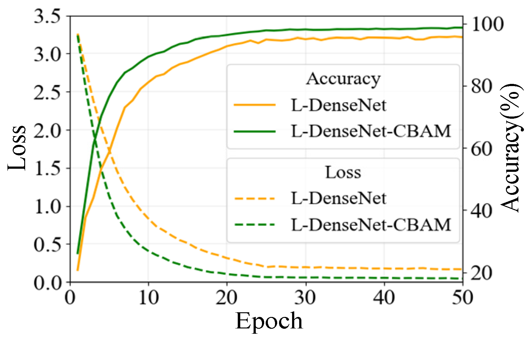
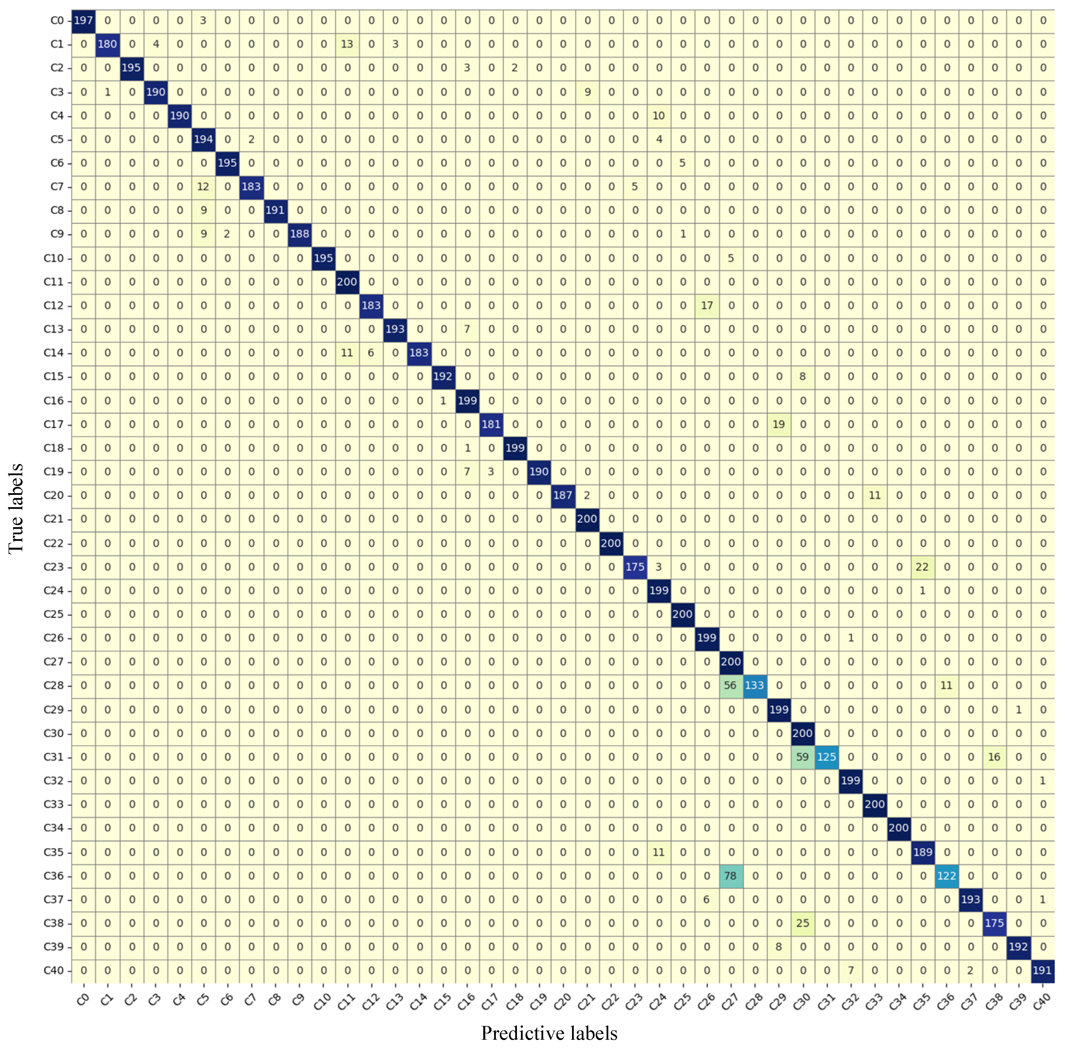
4.3. Classification Performance Evaluation of the Lightweight L-DenseNet-CBAM

To verify the performance of the proposed algorithm on the PQD classification task, we use the constructed LT image dataset of PQDs and rely on the same experimental environment. The L-DenseNet-CBAM model, which integrates the CBAM attention mechanism, and its skeleton network, L-DenseNet, which does not incorporate the CBAM module, are trained and tested. The classification accuracy and loss variation curves on the validation set during 50 training epochs are shown in Figure 6. Additionally, we evaluate the classification performance of both models under different SNR scenarios on the test set, as illustrated in

Table 4. Performance comparison of the two proposed models on the test set.

Model	Overall Classification Accuracy
	0 dB	60 dB	40 dB	20 dB
L-DenseNet	95.38	94.70	92.45	89.94
L-DenseNet-CBAM	98.83	98.05	96.18	93.86

.

As shown in Figure 6, the L-DenseNet-CBAM model, which integrates the attention mechanism module, exhibits significant improvements in both classification accuracy and convergence speed compared to L-DenseNet during the iterative training process. After reaching the convergent state, the accuracy and loss of the fusion model stabilize around 98.8% and 0.04, respectively, whereas the accuracy and loss of L-DenseNet fluctuate around 95.3% and 0.21. This indicates that while the skeleton model achieves relatively high PQD classification accuracy, the introduction of the CBAM module further enhances the ability of the classification network to extract fine-grained features of LT images corresponding to the PQD signals, thereby capturing the feature information in the input image more accurately.

In addition, as can be seen in Table 4, L-DenseNet-CBAM exhibits a significant advantage in PQD classification accuracy over L-DenseNet across four noise levels: 0 dB, 60 dB, 40 dB, and 20 dB, with classification accuracy on the test set improving by 3.45%, 3.35%, 3.73%, and 3.92%, respectively. This further demonstrates that integrating the CBAM attention mechanism between the dense connection learning module and the classification module enhances the model’s ability to capture key feature information, thereby achieving further improvement in the model classification performance.

4.4. Performance Comparison with Advanced PQD Classification Methods

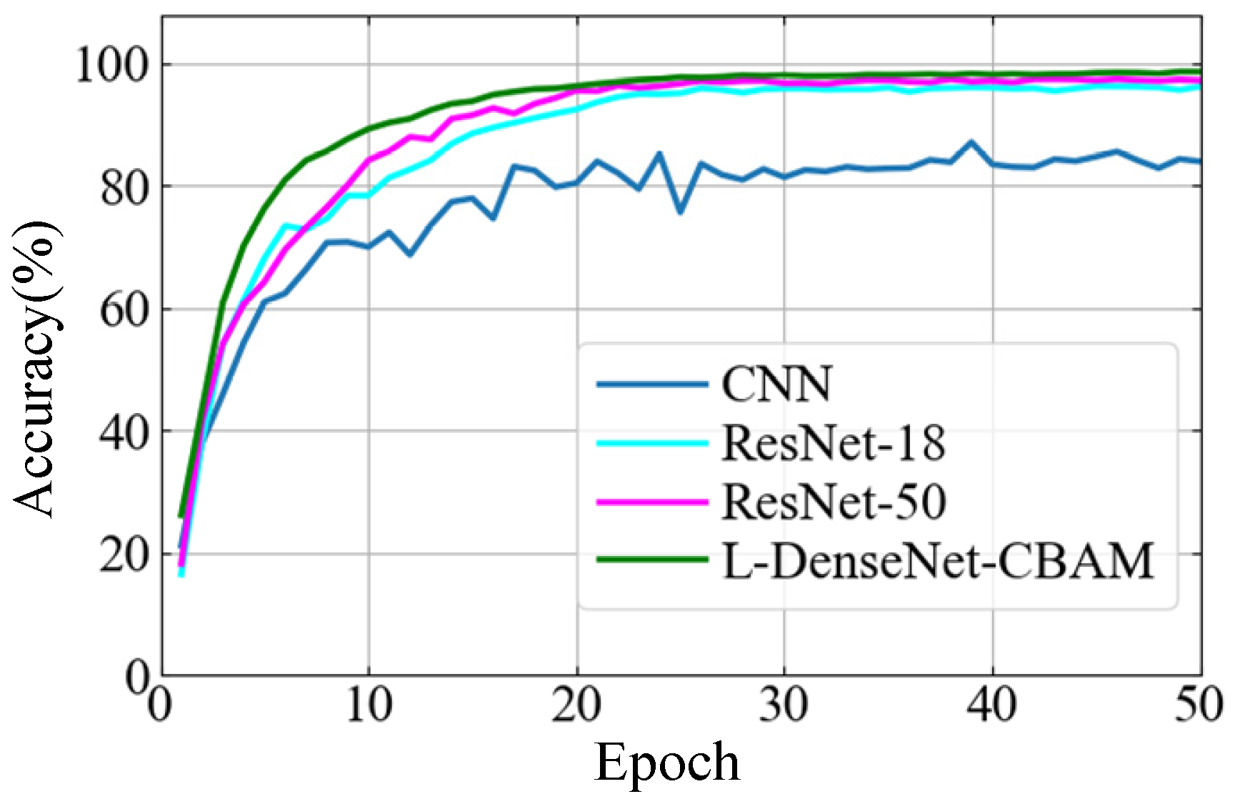
4.4.1. Performance Comparison with Advanced Image Recognition Models

To validate the advantages of the L-DenseNet-CBAM model in the PQD classification task, three advanced image classification networks that have been applied to PQD classification tasks, namely, CNN [11], ResNet-18 [12], and ResNet-50 [13], are selected as benchmark models for comparative analysis under the same LT dataset and experimental conditions. To accommodate the classification task in this paper, the number of neurons in the fully connected layers of the benchmark models is fine-tuned. The classification accuracy curves of each model on the validation set during training are shown in Figure 7, while the overall classification performance comparison on the test set is presented in

Table 5. Performance comparison of L-DenseNet-CBAM and existing advanced recognition networks on the test set.

Model	Overall Classification Accuracy
	0 dB	60 dB	40 dB	20 dB
CNN [11]	87.45	86.22	84.96	81.17
ResNet-18 [12]	96.52	95.85	94.51	91.22
ResNet-50 [13]	97.25	96.68	94.87	92.53
L-DenseNet-CBAM	98.83	98.05	96.18	93.86

. Note that, before being input into the network, the LT images need to be upsampled to 224 × 224 to meet the input size requirements of ResNet 18 and ResNet 50. Additionally, the images are resized to 200 × 200 to match the input specifications of the CNN model.

It can be seen in Figure 7 and Table 5 that CNN exhibits significantly lower classification performance during the training stage and on the test set compared to the other three models. This discrepancy is primarily due to the relatively simplified network architecture of CNN, which limits its ability to extract deep image feature information effectively. On the other hand, compared to the two ResNet models, the proposed fusion model demonstrates obvious advantages in learning efficiency during the early training stage and convergence speed, ultimately stabilizing at approximately 98.8%. In terms of performance on the test set, L-DenseNet-CBAM achieves higher overall classification accuracy than ResNet-18 and ResNet-50 under SNR levels of 0, 20, 40, and 60 dB, with improvements of 2.31%/1.58%, 2.20%/1.37%, 1.67%/1.31%, and 2.64%/1.33%, respectively. These results validate the superiority of the proposed fusion model in executing PQD classification tasks.

4.4.2. Performance Comparison with Advanced PQD Classification Algorithms

To further validate the superiority of the proposed algorithm framework in PQD classification, it is compared with eight published advanced classification algorithms, which are divided into machine learning-based algorithms and deep learning-based algorithms. The machine learning-based algorithms include DWT&SVM [6], ST&RF [7], and VMD&LGBM [8], which were originally designed for 10, 13, and 15 types of PQDs, respectively. The deep learning-based algorithms comprise FCN&LSTM [9] and DNN [10], which take one-dimensional signals as model inputs, as well as GAF&CNN [11], TC&ResNet18 [12], and ITC&ResNet50 [13], which convert one-dimensional signal sequences into two-dimensional images and then combine them with image recognition networks. These five deep learning-based algorithms target 12, 16, 17, 26, and 28 types of PQDs, respectively. To better align with practical measurement conditions in engineering applications, the performance of each algorithm is tested in a noise environment of 60 dB.

To ensure the fairness of each algorithm in the classification performance test, based on the same 41-type PQD signal dataset, each algorithm is used for signal processing and model training. Meanwhile, a hyperparameter optimization method based on grid search is adopted to solve the problem of parameter tuning difficulty caused by the complexity of the dataset to improve the overall algorithm performance. The sequential grid search, as detailed in [20], is used to determine the optimal parameters in turn. Compared with the global grid search, this approach significantly improves efficiency while maintaining the search quality. Accuracy is selected as the performance evaluation metric. The grid search results for the optimal hyperparameters are shown in

Table 6. Grid search results of optimal hyperparameters.

Model	Hyperparameters
	Item	Range	Values
SVM	Kernel	linear, poly, rbf, sigmoid	rbf
	Regulation parameter c	0.5, 1, 10, 100	1
	Gamma	Scale, auto	scale
RF	Criterion	gini, entropy	gini
	Decision tree number	400, 500, 600, 700	600
	The max depth	None, 5, 10, 20	None
LGBM	Estimator court	100, 200, 300, 400	200
	Max tree depth	1, 20, 50, 80	20
	Leave number	100, 200, 300, 400	100
	lambda	0, 100, 200, 300	200
FCN-LSTM	Batch size	16, 32, 64, 128	128
	Convolutional kernel size	(1,1), (3,3), (5,5)	(3,3)
	Number of neurons	128, 256, 512, 1024	512
	Optimizer	SGD, Adam, Nadam	Adam
	Dropout rate	0, 0.2, 0.4, 0.6	0.4
	Hidden activation function	ReLU, Tanh, Sigmoid	ReLU
DNN	Batch size	16, 32, 64, 128	32
	Convolutional kernel size	(1,1), (3,3), (5,5)	(3,3)
	Activation function	ReLU, Tanh, Sigmoid	Tanh
	BN layer	With or without	With
	Fully connected layer number	1, 2, 3, 4	3
	Optimizer	SGD, Adam, Nadam	Nadam
	Dropout rate	0, 0.2, 0.4, 0.6	0
CNN	Batch size	16, 32, 64, 128	64
	Convolutional kernel Size	(1,1), (3,3), (5,5)	(5,5)
	Activation function	ReLU, Tanh, Sigmoid	ReLU
	Fully connected layer number	1, 2, 3, 4	1
	Optimizer	SGD, Adam, Nadam	Adam
ResNet18	Batch size	16, 32, 64, 128	64
	Activation function	ReLU, Tanh, Sigmoid	ReLU
	The optimizer	SGD, Adam, Nadam	SGD
ResNet50	Batch size	16, 32, 64, 128	64
	Activation function	ReLU, Tanh, Sigmoid	ReLU
	The optimizer	SGD, Adam, Nadam	SGD
Proposal	Batch size	16, 32, 64, 128	64
	Activation function	ReLU, Tanh, Sigmoid	ReLU
	Optimizer	SGD, Adam, Nadam	Adam

. The comprehensive performance of each trained classification model on the test set is shown in

Table 7. Comprehensive performance comparison between the proposed algorithm and advanced classification algorithms in terms of accuracy and efficiency.

Algorithm	Params (M)	Size (MB)	FLOPs (G)	Time (ms)		Accuracy
				Signal Processing (ms)	Model Classification (ms)
DWT&SVM [6]	10.92	85.65	32.72	16.83	13.82	88.75
ST&RF [7]	/	1014.17	/	59.44	29.38	84.91
VMD&LGBM [8]	/	7.29	/	24.26	11.94	89.28
FCN-LSTM [9]	1.72	6.58	0.54	/	18.37	77.51
DNN [10]	0.17	0.64	0.11	/	16.43	90.23
GAF&CNN [11]	1.53	5.83	0.13	109.93	9.64	91.56
TC&ResNet18 [12]	11.19	42.73	1.82	34.75	41.90	95.63
ITC&ResNet50 [13]	23.57	90.11	4.13	57.71	74.33	96.78
Proposed	1.88	6.94	0.22	12.26	11.06	98.05

. Here, time refers to the average time taken by each algorithm to classify a signal sample in the test set, including signal processing time and model classification time.

It can be seen in Table 7 that for 41 types of complex PQD datasets, which incorporate up to four distinct and intertwined single disturbances within the same waveform, the accuracy of machine learning-based algorithms does not exceed 90%. This is mainly because, for highly nonlinear and dynamically changing complex composite disturbance signals, the manual feature extraction methods designed based on expert experience cannot fully extract high-order coupling features, resulting in insufficient generalization performance and limiting its accuracy performance. Meanwhile, in terms of efficiency performance, since the manual feature extraction methods generally need to perform complex time-frequency feature decoupling and high-dimensional component separation operations, their signal processing efficiency is lower than that of the proposed LT because the latter only needs to construct an ideal signal for simple curve synthesis. Furthermore, due to the lightweight architecture design of L-DenseNet-CBAM, its classification efficiency is also higher than that of the three machine learning classifiers. One-dimensional deep learning algorithms directly take sequence data as model input without any data processing, thus outperforming other algorithms in terms of efficiency performance. However, their limitations in information mining of complex temporal sequence data still constrain their recognition accuracy for complex PQDs. Based on the deep feature mining capabilities and strong generalization of image recognition networks, the accuracy performance metrics of two-dimensional deep learning algorithms are superior to those of machine learning-based algorithms and one-dimensional deep learning algorithms. The proposed algorithm can achieve a classification accuracy of 98.05%, significantly outperforming GAF&CNN, TC&ResNet18, and ITC&ResNet50. In addition, due to the rapidity of data conversion and the lightweight design of the model structure, the total time for converting and classifying a signal sample is only 23.32 ms, fully meeting the real-time performance requirements of real-world PQ monitoring data analysis.

4.5. Noise Robustness Performance Evaluation

Noise environments can easily distort PQD signals, interfering with the algorithm’s ability to accurately identify their true types and leading to a decline in classification performance. Therefore, to evaluate the anti-noise capability of the algorithm, based on the classification performance results of the model in different SNR environments, as shown in Table 4, the specific classification effects on various disturbances are tested in a strong noise environment of 20 dB. The test results and their corresponding confusion matrix are presented in

Table 8. Classification results of the proposed algorithm in the 20 dB SNR environment.

Label	Type	Accuracy	Label	Type	Accuracy
C0	Normal	98.5%	C21	Interr + Oscill	100%
C1	Sag	90%	C22	Interr + Notch	100%
C2	Swell	97.5%	C23	Har + Flicker	87.5%
C3	Interruption	95%	C24	Har + Oscill	99.5%
C4	Harmonic	95%	C25	Pulse + Flicker	100%
C5	Oscillatory transient	97%	C26	Sag + Pulse + Flicker	99.5%
C6	Pulse	97.5%	C27	Sag + Har + Oscill	100%
C7	Flicker	91.5%	C28	Sag + Har + Flicker	66.5%
C8	Notch	95.5%	C29	Swell + Pulse + Flicker	99.5%
C9	Spike	94%	C30	Swell + Har + Oscill	100%
C10	Sag + Har	97.5%	C31	Swell + Har + Flicker	62.5%
C11	Sag + Oscil	100%	C32	Interr + Pulse + Flicker	99.5%
C12	Sag + Pulse	91.5%	C33	Interr + Har + Oscill	100%
C13	Sag + Notch	96.5%	C34	Har + Pulse + Flicker	100%
C14	Sag + Spike	91.5%	C35	Har + Oscill + Flicker	94.5%
C15	Swell + Har	96%	C36	Sag + Har + Oscill + Flicker	61%
C16	Swell + Oscill	99.5%	C37	Sag + Har + Pulse + Flicker	96.5%
C17	Swell + Pulse	90.5%	C38	Swell + Har + Oscill + Flicker	87.5%
C18	Swell + Notch	99.5%	C39	Swell + Har + Pulse + Flicker	96%
C19	Swell + Spike	95%	C40	Interr + Har + Pulse + Flicker	95.5%
C20	Interr + Har	93.5%	Overall Accuracy		93.86%

Note that since the names interruption, harmonic, and oscillatory transient are relatively long, they are abbreviated as Interr, Har, and Oscill when describing composite disturbances.

and Figure 8, respectively.

As can be seen in Figure 8 and Table 8, the recognition rate of C0-Normal has not reached 100%. This is mainly because, in a 20 dB strong noise environment, the noise interference causes relatively severe distortion of the signal waveform, resulting in high-frequency fluctuations in its amplitude. In other words, the corresponding LT deformation characteristics of C0 are similar to those of C5-Oscillatory transient. Therefore, three groups of samples are identified as C5. Meanwhile, due to the presence of clearly distinguishable amplitude deviation components (C1/C2/C3) and C5 and C8, three groups of double disturbances (C11/C21/C22) can be identified with 100% accuracy. On this basis, three triple disturbances involving C4 (C27/C30/C33), which also have excellent feature representation capabilities in strong noise environments, can likewise achieve 100% classification accuracy. In addition, the samples of C25 and C34 are accurately classified due to the presence of clearly characterized C6-pulse and C7-Flicker, which have similar features to C5 in a strong noise environment. On the other hand, the proposed algorithm performs poorly in the classification of C28, C31, and C36, with classification accuracies below 70%. This is mainly because the waveform fluctuation characteristics of C7 under a strong noise environment of 20 dB are highly similar to those of C5. When both appear on the same waveform, the characteristics of the former are easily masked by the latter, thereby causing confusion in determination. Therefore, 56 and 11 groups of samples in C28 are misclassified as C27 and C36, respectively, 59 and 16 groups of samples in C31 are determined as C30 and C38, respectively, and 78 groups of samples in C36 are confused as C27.

Overall, despite certain accuracy limitations for specific disturbance types in a strong noise environment of 20 dB, the proposed algorithm framework still achieves an overall PQD classification accuracy of 93.86%, demonstrating excellent classification performance and noise robustness.

5. Case Studies: Part II: Real-World Measured Data Analysis

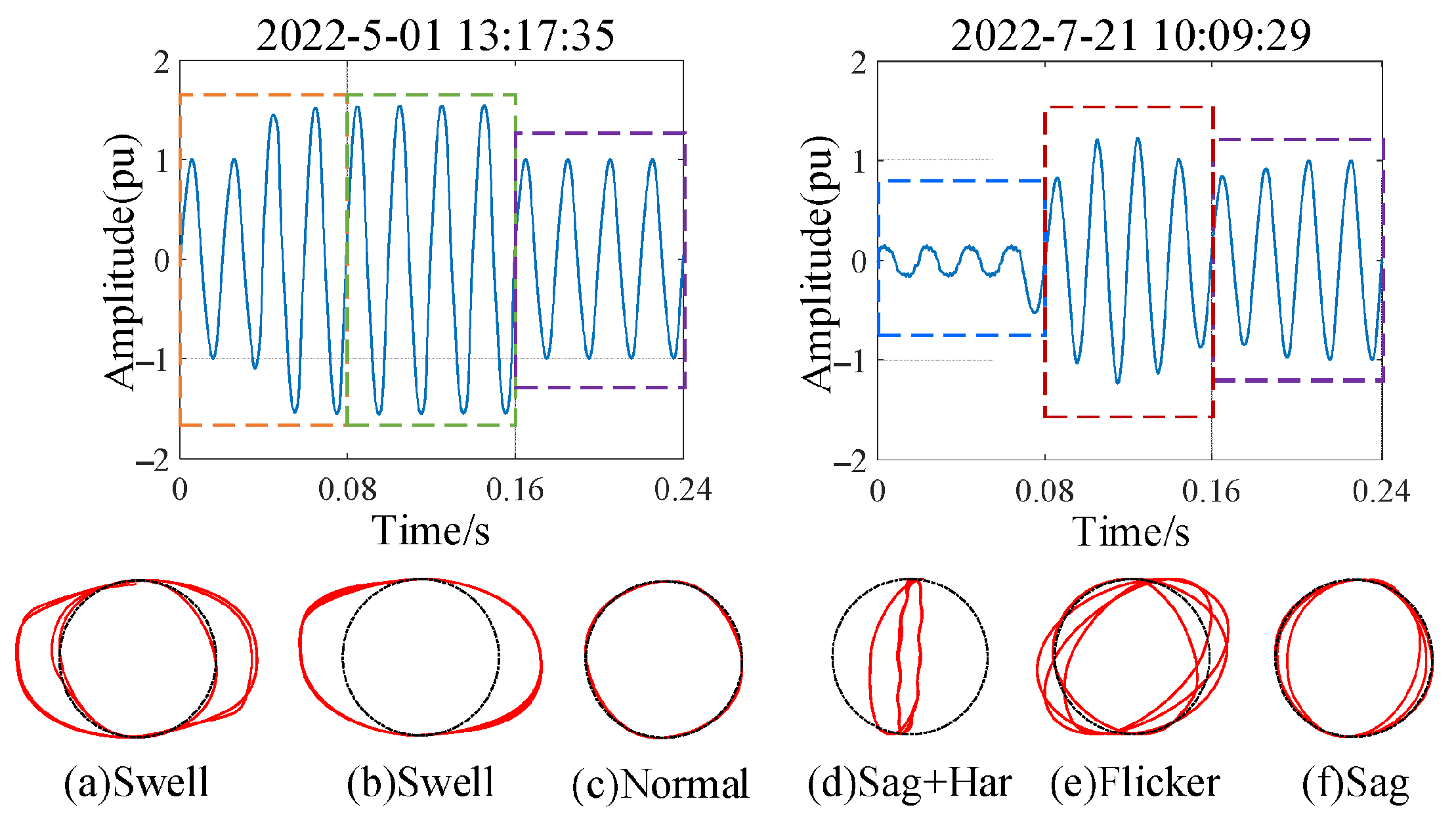
5.1. Engineering Effectiveness Analysis of the Proposed PQD Classification Algorithm

To verify the effectiveness of the proposed algorithm in practical engineering applications, classification performance tests are conducted using measured disturbance signal data collected from PQ monitoring sensors at a 10 kV substation in the southern Jiangsu power grid, China. The nominal frequency of the system is 50 Hz, and the sampling rate of the PQ monitoring sensor is 12.8 kHz, meaning that one sample point is recorded every 78 μs. To verify the classification performance of the proposed algorithm for continuous sliding window sample slices, each collected signal waveform sample has a duration of 0.24 s (12 cycles), resulting in a total of 69 signal samples. Since slicing is performed every four cycles, a total of 207 disturbance signal samples are included in the test. To meet the input requirements of the proposed image classification model, each waveform sample is normalized and sliced every four cycles. Meanwhile, according to the LT conversion process in Section 2.2, the ideal reference signal is constructed through (2) and combined with the target slice sample, which are respectively used as the Y-axis and X-axis of the Cartesian coordinate system for Lissajous curve synthesis, thereby generating the LT representations of the measured disturbance signals. The real-world measured waveforms and their sliced LT representation for typical PQDs are shown in Figure 9. It can be observed that the LT corresponding to the measured disturbance signals still exhibits morphological characteristics similar to the trajectories of standard signals, demonstrating that LT conversion maintains excellent feature representation capability for measured signal data. To better reflect real-world measurement conditions, we retain the optimal L-DenseNet-CBAM trained model in the 60 dB SNR environment and classify all LT samples corresponding to the measured signals, with the results presented in

Table 9. Classification results of PQD measured signals using LT+L-DenseNet-CBAM.

Label	Type of PQDs	Number of Samples	Classification Results
C1	Sag	68	C1: 61/C3: 2/C1 + C5: 4/C1 + C8: 1
C2	Swell	25	C2: 25
C3	Interruption	3	C3: 3
C4	Harmonic	24	C4: 23/C4 + C5: 1
C6	Pulse	5	C6: 5
C7	Flicker	34	C7: 30/C4 + C7: 3/C6 + C7: 1
C1 + C4	Sag + Har	18	C1 + C4: 16/C1: 2
C1 + C5	Sag + Oscill	12	C1 + C5: 9/C1 + C4: 2/C1 + C4 + C5: 1
C6 + C7	Pulse + Flicker	5	C6 + C7: 5
C2 + C9	Swell + Spike	5	C2 + C9: 5
C1 + C4 + C7	Sag + Har + Flicker	5	C1 + C4 + C7: 5
C3 + C4 + C5	Interr + Har + Oscill	3	C3 + C4 + C5: 2/C1 + C4: 1

.

It can be seen in Table 9 that in terms of single disturbance classification performance, the proposed algorithm demonstrates excellent accuracy for disturbance types C2, C3, C4, and C5, while partial confusion occurs for C1 and C7. Specifically, for the C1-Sag type, two samples are misclassified as interruptions due to their large voltage drop amplitude, which is close to the critical threshold between sag and interruption. Meanwhile, due to the influence of environmental noise, four groups of samples are determined to contain oscillatory transients. Furthermore, due to the widespread integration of power electronic devices and nonlinear loads in practical power systems, high-order harmonics are continuously injected during operation, resulting in certain distortions in voltage waveforms. Consequently, one sample is identified as Sag + Notch. Similarly, for the C7-Flicker, the introduction of high-order harmonics leads to three samples being recognized as double disturbances involving harmonic components. Moreover, one sample is detected as containing a pulse component due to the presence of a severe noise point. In terms of the classification of compound disturbances with more complex signal fluctuation characteristics, due to the distortion interference from environmental noise and injected harmonics on the PQD signal waveform, there are a total of five groups of samples in the C1 + C4/C1 + C5 types with determination confusion, resulting in certain classification deviations. In the case of C3 + C4 + C5, one sample with a voltage drop amplitude near the critical threshold and a low-magnitude, short-duration oscillatory component is misclassified as C1 + C4. In summary, due to factors such as environmental noise, operational conditions, and measurement errors, real-world disturbance signals exhibit greater complexity and coupling than ideal simulated signals, posing a significant challenge for accurate classification. Nevertheless, the proposed algorithm achieves a high classification accuracy of 91.30% on complex real-world measured disturbance signals, thereby verifying its effectiveness and reliability in practical engineering applications.

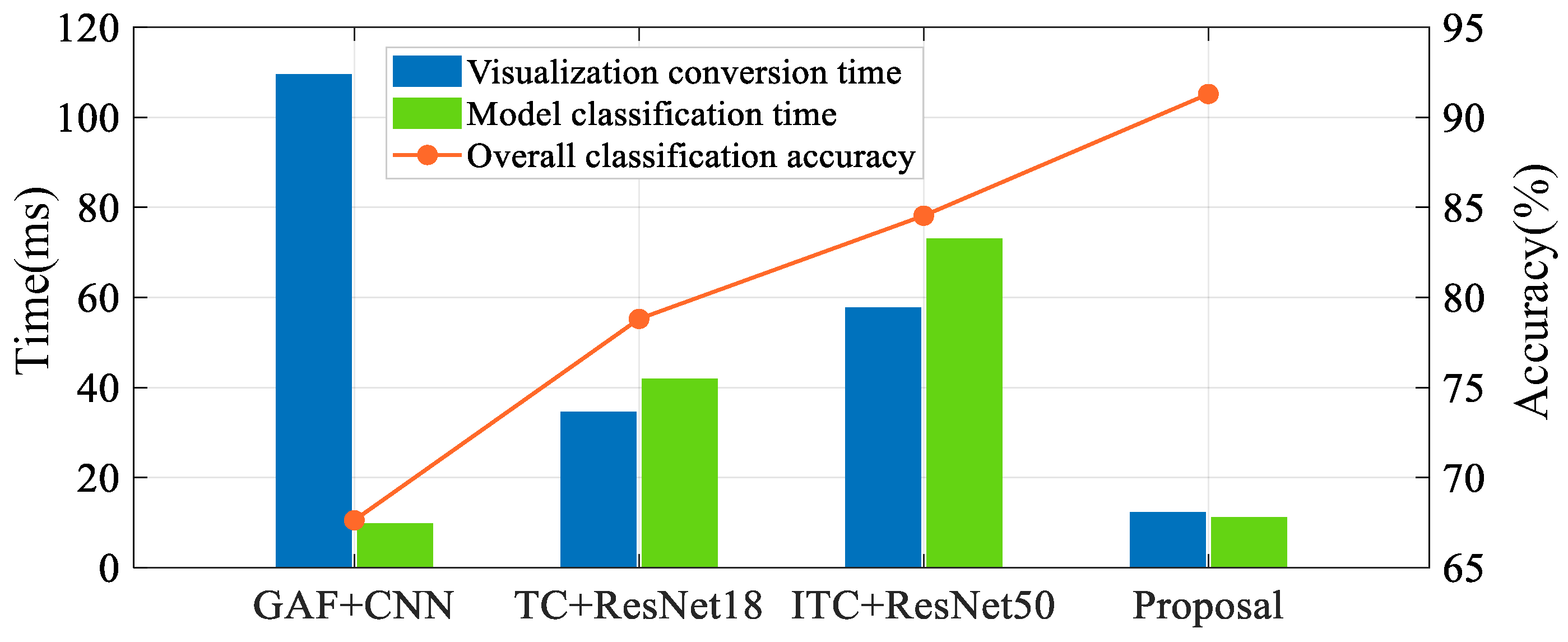
5.2. Comprehensive Performance Comparison with the Existing PQD Classification Algorithms

In order to further verify the superiority of the proposed algorithm in the PQD classification task of engineering practice, we select the top three existing PQD classification algorithms ranked by accuracy performance in Section 4.4.2: GAF + CNN [11], TC + ResNet-18 [12], and ITC + ResNet-50 [13]. These serve as benchmark algorithms for performance comparison. Among them, the size of the sequence visualization images remains consistent with the original settings, while the hyperparameters of the classification network are configured identically to those in this paper. Under the same experimental conditions, 41 types of PQDs are generated, with 1000 samples per type for the GAF, TC, and ITC image datasets, which are divided in the same proportions and used as inputs for the classification network. After training the CNN, ResNet-18 and ResNet-50 classification networks and obtaining the models that perform best on the validation set, they are respectively applied to the GAF, TC, and ITC image datasets converted from real-world measured signals. The classification results are then comprehensively compared with those of the proposed algorithm, as shown in Figure 10 and

Table 10. Comprehensive performance evaluation metrics of various PQD classification algorithms.

Algorithm	Visualization Conversion Time	Model Classification Time	Accuracy
GAF + CNN [11]	109.55 ms	9.76 ms	67.63%
TC + ResNet18 [12]	34.58 ms	41.95 ms	78.81%
ITC + ResNet50 [13]	57.78 ms	73.05 ms	84.54%
Proposal	12.26 ms	11.22 ms	91.30%

. The times for visualization conversion and model classification are both the average durations obtained from 50 consecutive tests for a signal sample.

It can be seen that in terms of classification accuracy, since GAF is prone to losing important feature information, such as signal amplitude, during the encoding process, and the real-time signal state changes are more complex, while the depth of the CNN network is relatively shallow and unable to capture the deep semantic information of the image. As a result, the overall classification accuracy is only 67.63%. During signal visualization, TC exhibits significant curve jumps and endpoint effects, which interfere with the classification network’s ability to capture essential feature information, thereby reducing the model’s classification performance. As an improved version of TC, ITC effectively eliminates curve jumps and endpoint effects using ESM. However, this method tends to cause the loss of envelope feature information during signal processing. As a result, its accuracy is also limited. In terms of classification efficiency, the proposed algorithm significantly outperforms other methods in visualization transformation efficiency due to the simplicity of the LT conversion process, which requires only the construction of an ideal reference signal. Additionally, due to its lightweight structural design, the model achieves higher classification efficiency compared to the larger-scale ResNet-18/ResNet-50. However, its performance is slightly inferior to that of CNN, as CNN has lower Params, FLOPs, and a smaller model size, making it structurally simpler. Nevertheless, the inherent accuracy limitations caused by its weaker feature extraction capability may render it unsuitable for practical engineering PQD classification tasks. Thus, the effectiveness and superiority of the proposed LT + L-DenseNet-CBAM framework in real-world measured PQD classification tasks have been fully validated. With the increasing deployment of power electronic devices leading to a massive growth in PQ monitoring data, the proposed scheme can further enhance PQD data processing and classification efficiency, thereby achieving real-time situational awareness of the power system’s health status and providing crucial support for the subsequent timely adoption of effective solutions.

6. Conclusions

To address the challenge of the difficulty associated with achieving accurate and rapid classification of complex PQDs in the context of modern power systems, this paper proposes an efficient PQD classification algorithm based on LT and lightweight DenseNet. Firstly, based on the concept of Lissajous curves, an ideal signal is constructed and combined with a disturbance signal to form a trajectory curve with distinct and easily identifiable features, thereby enhancing visualization efficiency while concretizing temporal characteristics. Secondly, a lightweight L-DenseNet architecture with a dense connection mechanism is designed to improve the comprehensiveness of feature extraction and enhance classification efficiency. Furthermore, by introducing the CBAM attention mechanism, the performance of L-DenseNet in capturing trajectory feature information has been further optimized. The simulation experimental results demonstrate that for a dataset of 41 types of complex PQD containing up to four types of single disturbances superimposed on the same waveform, compared with the existing eight advanced PQD classification algorithms, the proposed framework achieves optimal overall performance in terms of classification accuracy and efficiency. In a 60 dB noise environment, the proposed framework achieves an accuracy of 98.08% and requires only 23.32 ms to classify a signal sample. Compared with the existing most advanced ITC + ResNet-50, it improves accuracy by 1.27% and reduces classification time by 82.34%. Furthermore, the measured disturbance signal experiments at the grid substation show that LT + L-DenseNet-CBAM can achieve a classification accuracy of 91.30% and a processing time of just 23.48 ms on the measured PQD signal set, which has more complex coupling characteristics. Relative to ITC + ResNet-50, these results represent improvements of 6.76% in accuracy and 82.05% in efficiency, thereby confirming the proposed algorithm’s effectiveness and superiority in PQD classification tasks. It fully meets the high-performance requirements of the power grid operation and maintenance department for processing and analyzing massive PQ monitoring data.

In the future, we will focus on addressing three challenges: (1) When processing real-world disturbance signals with more complex fluctuation patterns, the classification accuracy of the proposed algorithm still has room for improvement. Subsequently, more abundant on-site measured disturbance data need to be collected from engineering practice to further enhance the generalization performance of the algorithm. (2) The second challenge involves exploring edge computing-based PQD classification solutions by deploying the trained lightweight classification network on edge platforms that are closer to device terminals but resource-constrained. This will further improve the efficiency performance of PQ situational awareness. (3) The third challenge involves investigating frequency distortion-related PQDs. Future efforts will focus on identifying representative frequency distortion patterns and integrating adaptive signal processing techniques to improve detection sensitivity. This line of research will enhance the algorithm’s robustness in scenarios in which fundamental frequency deviations interact with other disturbance components, especially under the evolving conditions of modern power systems.

References

1. Chakraborty, S.; Modi, G.; Singh, B. A Cost Optimized-Reliable-Resilient-Realtime- Rule-Based Energy Management Scheme for a SPV-BES-Based Microgrid for Smart Building Applications. IEEE Trans. Smart Grid 2023, 14, 2572–2581. [Google Scholar] [CrossRef]
2. Vasquez, J.; Jaramillo, M.; Carrión, D. An Intelligent Framework for Multiscale Detection of Power System Events Using Hilbert–Huang Decomposition and Neural Classifiers. Appl. Sci. 2025, 15, 6404. [Google Scholar] [CrossRef]
3. Mendia, J. Power Quality Monitoring Part 1: The importance of standards compliant power quality measurements. Analog. Dialogue 2022, 56, 1–4. [Google Scholar]
4. IEEE Std 2938 TM-2023; IEEE Guide for Economic Loss Evaluation of Sensitive Industrial Customers Caused by Voltage Sags. IEEE Power and Energy Society: Piscataway, NJ, USA, 2023.
5. Ptak, T.; Brooks, J.; Stock, R. A systematic review and typology of power outage literature: Critical infrastructure, climate change and social impacts. Renew. Sustain. Energy Rev. 2025, 218, 115778. [Google Scholar] [CrossRef]
6. Borras, M.; Bravo, J.; Montano, J. Disturbance ratio for optimal multi-event classification in power distribution networks. IEEE Trans. Ind. Electron. 2016, 63, 3117–3124. [Google Scholar] [CrossRef]
7. Reddy, V.; Sodhi, R. A modified S-transform and random forests-based power quality assessment framework. IEEE Trans. Instrum. Meas. 2018, 67, 78–89. [Google Scholar] [CrossRef]
8. Mishra, S.; Mallick, R.K.; Gadanayak, D.A.; Nayak, P.; Sharma, R.; Panda, G.; Al-Numay, M.S.; Siano, P. Real time intelligent detection of PQ disturbances with variational mode energy features and hybrid optimized light GBM classifier. IEEE Access 2024, 12, 47155–47172. [Google Scholar] [CrossRef]
9. Xu, W.; Duan, C.; Wang, X.; Dai, J. Power Quality Disturbance Identification Method Based on Improved Fully Convolutional Network. In Proceedings of the 2022 5th Asia Conference on Energy and Electrical Engineering (ACEEE), Kuala Lumpur, Malaysia, 8–10 July 2022; pp. 1–6. [Google Scholar]
10. Wang, S.; Chen, H. A novel deep learning method for the classification of power quality disturbances using deep convolutional neural network. Appl. Energy 2019, 235, 1126–1140. [Google Scholar] [CrossRef]
11. Shukla, J.; Panigrahi, B.; Ray, P. Power quality disturbances classification based on Gramian angular summation field method and convolutional neural networks. Int. Trans. Electr. Energy Syst. 2021, 31, e13222. [Google Scholar] [CrossRef]
12. Lan, M.; Liu, Y.; Jin, T.; Gong, Z.; Liu, Z. An improved recognition method based on visual trajectory circle and ResNet18 for complex power quality disturbances. Proc. CSEE 2022, 42, 6274–6285. [Google Scholar]
13. Yuan, D.; Liu, Y.; Hu, H.; Lan, M.; Jin, T.; Mohamed, M. A Novel Recognition Method for Complex Power Quality Disturbances Based on Visualization Trajectory Circle and Machine Vision. IEEE Trans. Instrum. Meas. 2022, 71, 1–13. [Google Scholar] [CrossRef]
14. IEEE Std 1159 TM-2019; IEEE Recommended Practice for Monitoring Electric Power Quality. IEEE: Washington, DC, USA, 2019.
15. Karacor, D.; Nazlibilek, S.; Sazli, M.; Akarsu, E. Discrete Lissajous figures and applications. IEEE Trans. Instrum. Meas. 2014, 63, 2963–2972. [Google Scholar] [CrossRef]
16. Abu-Siada, A.; Mir, S. A new on-line technique to identify fault location within long transmission lines. Eng. Fail. Anal. 2019, 105, 52–64. [Google Scholar] [CrossRef]
17. Izad, M.; Mohsenian-Rad, H. A Synchronized Lissajous-Based Method to Detect and Classify Events in Synchro-Waveform Measurements in Power Distribution Networks. IEEE Trans. Smart Grid 2022, 13, 2170–2184. [Google Scholar] [CrossRef]
18. Huang, G.; Liu, Z.; LAURENS, V. Densely connected convolutional networks. In Proceedings of the 2017 IEEE Conference on Computer Vision and Pattern Recognition(CVPR), Honolulu, HI, USA, 21–26 July 2017; pp. 2261–2269. [Google Scholar]
19. Woo, S.; Park, J.; LEE, J. CBAM: Convolutional block attention module. In Proceedings of the 15th European Conference on Computer Vision (ECCV), Munich, Germany, 8–14 September 2018; pp. 3–19. [Google Scholar]
20. Takiddin, A.; Ismail, M.; Zafar, U.; Serpedin, E. Deep autoencoder based anomaly detection of electricity theft cyberattacks in smart grids. IEEE Syst. J. 2022, 16, 4106–4117. [Google Scholar] [CrossRef]
Figure 2. Lissajous trajectories of PQD signals. The red lines represent the LT corresponding to PQDs with waveform distortion, while the dotted lines indicate the LT corresponding to normal signal waveforms.
Applsci 15 08021 g002
Figure 1. Signal waveforms of PQDs.
Applsci 15 08021 g001
Figure 3. Structure of the dense connected block.
Applsci 15 08021 g003
Figure 4. Structure of the CBAM attention mechanism module.
Applsci 15 08021 g004
Figure 6. Training performance of L-DenseNet with/without CBAM on the validation set.
Applsci 15 08021 g006
Figure 7. Accuracy performance comparison of L-DenseNet-CBAM and advanced image recognition networks on the validation set.
Applsci 15 08021 g007
Figure 8. Confusion matrix of 41 types of PQD classification results in a strong noise environment of 20 dB. The background color indicates the quantity of classification results; the darker the color, the greater the number of samples in the corresponding category.
Applsci 15 08021 g008
Figure 9. Measured waveforms and their Lissajous trajectories for typical PQDs. The red lines represent the LT corresponding to PQDs with waveform distortion, while the dotted lines indicate the LT corresponding to normal signal waveforms.
Applsci 15 08021 g009
Figure 10. Comparison of accuracy and efficiency performance between the proposed algorithm and three advanced deep learning algorithms.
Applsci 15 08021 g010