
CoTD-VAE: Interpretable Disentanglement of Static, Trend, and Event Components in Complex Time Series for Medical Applications


Abstract
1. Introduction
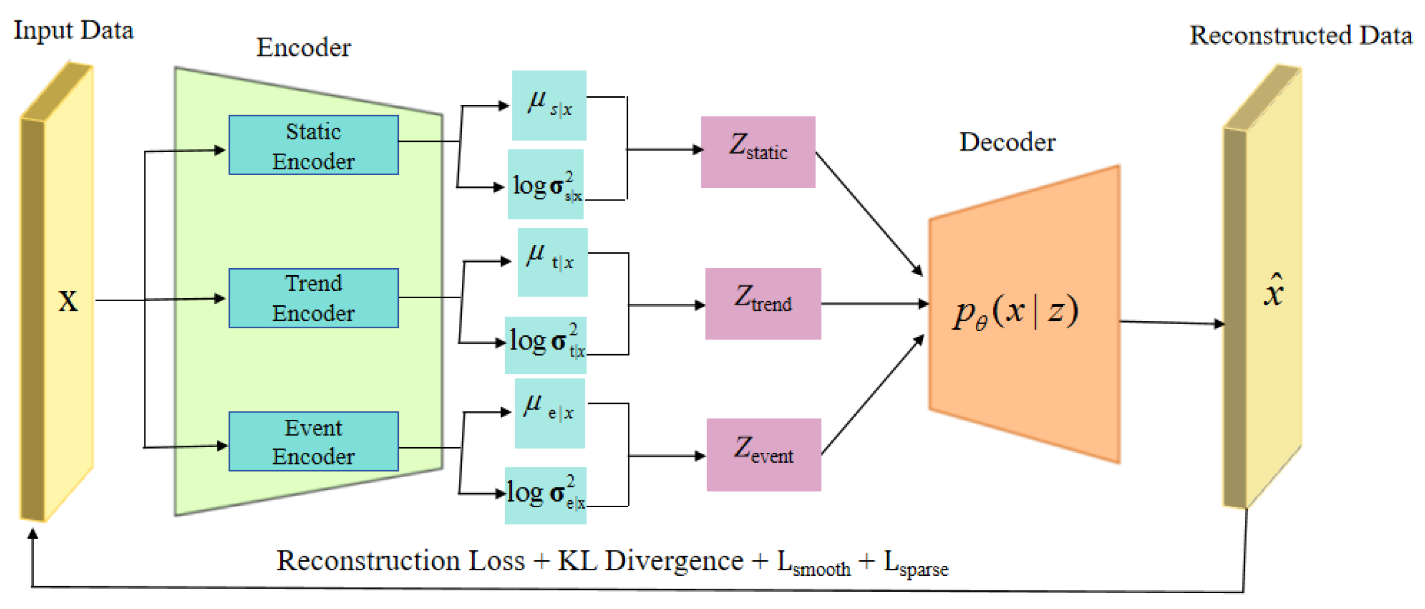
- We propose a novel disentangled variational autoencoder called “CoTD-VAE”. It can disentangle medical time series data into three parts: static, trend, and event.
- CoTD-VAE is given explicit temporal constraints, which are the loss of trend smoothness and the loss of event sparsity. These constraints improve the model’s ability to capture and distinguish dynamic changes in medical data at different timescales.
- We evaluated the proposed CoTD-VAE and its learned Disentangled representation by running an experiment on a real healthcare risk prediction task. The results of the experiment showed that the proposed CoTD-VAE and its learned Disentangled representation are valid and better than other models.
2. Related Work
2.1. Medical Time Series Analysis
2.2. Disentangled Representation Learning
2.3. Disentangled Representation Learning for Time Series Based on LSTM, Transformer and VAE
3. Methods
4. Experiments
4.1. Datasets
4.2. Baselines
4.3. Ablation Experiments
- No Smoothness: It would be beneficial to consider removing the loss of trend smoothing and testing the impact of the trend smoothing constraints on the model performance.
- No Sparsity: It might be worthwhile to explore removing the loss of event sparsity and testing the impact of the event sparsity constraints on the model performance. By comparing the performance difference between these variants and the full model, we can hopefully quantify the contribution of these two components to the overall performance and verify the validity of our proposed temporal constraints.
5. Results
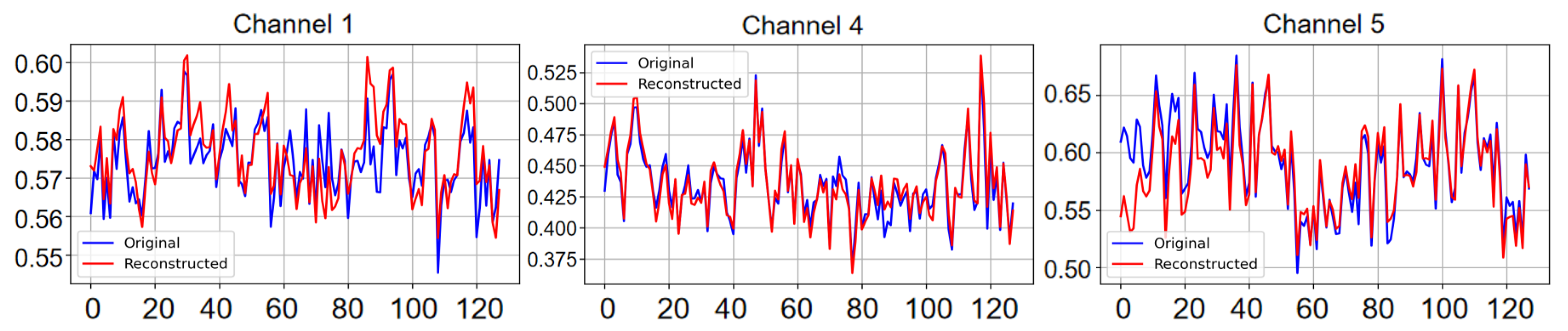
5.1. Reconstruction Task
5.2. Classification Task
5.3. Ablation and Sensitivity Analysis
5.3.1. Ablation Study
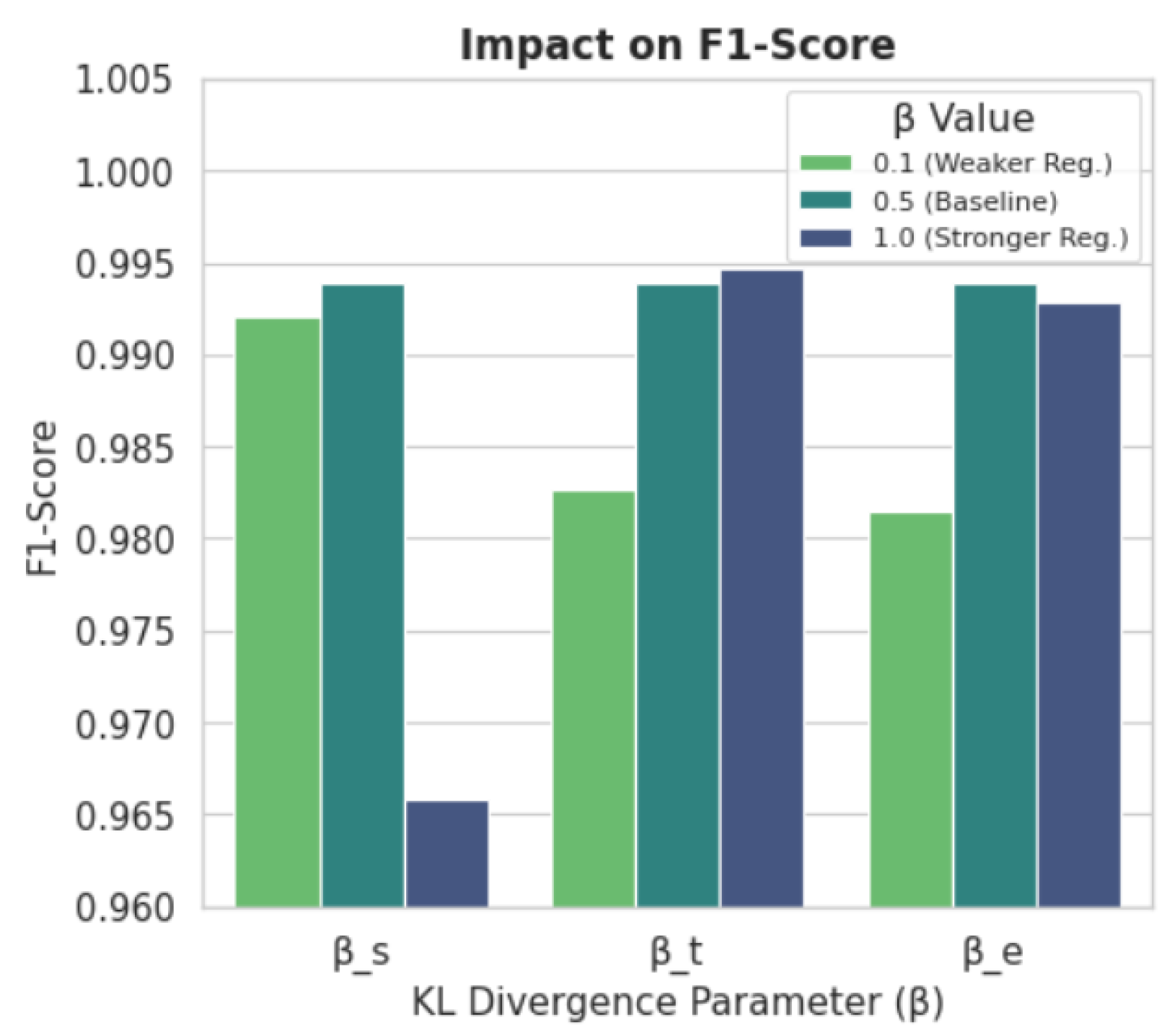
5.3.2. Sensitivity Analysis
5.4. Interpretability Analysis
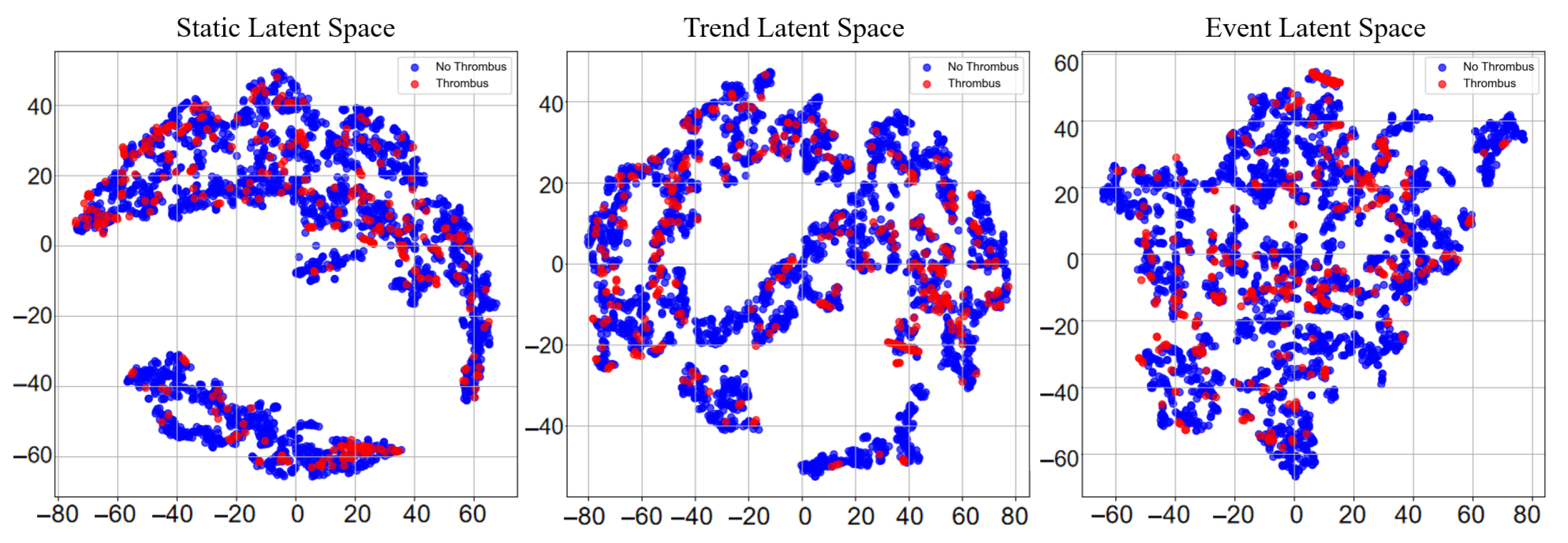
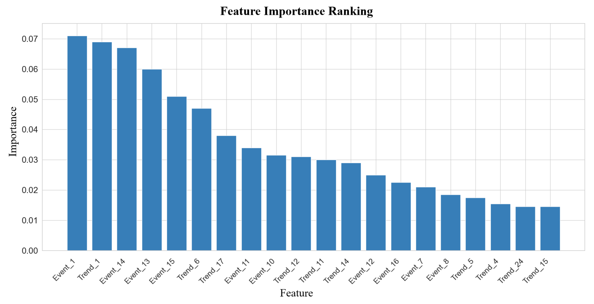
5.4.1. Clinical Decision Insight from MIMIC-IV
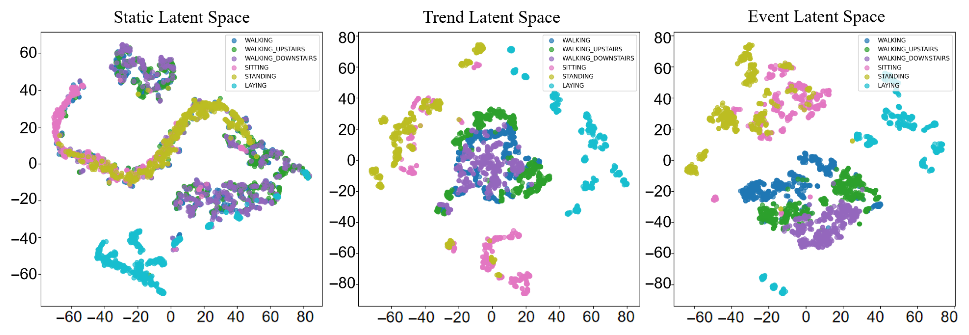
5.4.2. Representation Validation on UCI HAR
6. Discussion
7. Conclusions
- Further optimization of model architecture: Exploring more advanced sequence modeling architectures (e.g., more complex attention mechanisms) or different disentanglement methods to further enhance the separability and expressiveness of latent representations. Also, investigating how to adaptively determine the dimensions of each latent space and the weights of the regularization terms (e.g., the and parameters) instead of using fixed hyperparameter settings.
- More fine-grained latent factor analysis and clinical association: Conducting more in-depth analysis of the disentangled static, trend, and event latent spaces, for example, by using clustering, visualization, or other statistical methods, to identify clinically meaningful subgroups or patterns. Crucially, future work will involve close collaboration with clinical experts to validate the specific interpretations of these learned latent factors and to assess their association strength with specific disease states or risk events.
- Application to wider medical time series tasks: Applying the CoTD-VAE model to other types of medical time series data (e.g., physiological waveforms, continuous glucose monitoring data, etc.), as well as different clinical tasks, such as early disease diagnosis, disease progression prediction, treatment response assessment, or patient phenotyping.
- Enhancing model generalization ability and transferability: Investigating how to improve the generalization ability of trained models across different hospitals or patient populations. Exploring federated learning or transfer learning techniques in order to utilize data from multiple sources while protecting data privacy, aiming to train more robust models.
- Integration with causal inference: Exploring the combination of disentangled representations with causal inference methods to better understand the causal relationships between different latent factors and how they jointly influence patient risk outcomes. This will help reveal the underlying disease mechanisms and provide guidance for clinical interventions.
Author Contributions
Funding
Institutional Review Board Statement
Informed Consent Statement
Data Availability Statement
Conflicts of Interest
Appendix A. Sensitivity Analysis Results

| Parameter Tested | Value | Accuracy | Precision | Recall | F1-Score | AUC |
|---|---|---|---|---|---|---|
| Baseline Config | – | 0.9981 | 1.0000 | 0.9878 | 0.9939 | 1.0000 |
| learning_rate | 1 × 10⁻³ | 0.9980 | 1.0000 | 0.9875 | 0.9937 | 1.0000 |
| 1 × 10⁻⁴ | 0.9969 | 0.9997 | 0.9804 | 0.9899 | 1.0000 | |
| 0.1 | 0.9976 | 1.0000 | 0.9849 | 0.9924 | 1.0000 | |
| 1.0 | 0.9985 | 1.0000 | 0.9904 | 0.9952 | 1.0000 | |
| 0.1 | 0.9975 | 1.0000 | 0.9842 | 0.9921 | 1.0000 | |
| 0.5 | 0.9978 | 1.0000 | 0.9862 | 0.9930 | 1.0000 | |
| 0.1 | 0.9980 | 1.0000 | 0.9871 | 0.9935 | 1.0000 | |
| 0.5 | 0.9976 | 1.0000 | 0.9846 | 0.9922 | 1.0000 | |
| 0.1 | 0.9975 | 1.0000 | 0.9842 | 0.9921 | 1.0000 | |
| 1.0 | 0.9896 | 1.0000 | 0.9341 | 0.9659 | 1.0000 | |
| 0.1 | 0.9946 | 1.0000 | 0.9659 | 0.9827 | 1.0000 | |
| 1.0 | 0.9983 | 1.0000 | 0.9894 | 0.9947 | 1.0000 | |
| 0.1 | 0.9943 | 1.0000 | 0.9637 | 0.9815 | 0.9999 | |
| 1.0 | 0.9978 | 1.0000 | 0.9859 | 0.9929 | 1.0000 |
References
- Sakib, M.; Mustajab, S.; Alam, M. Ensemble deep learning techniques for time series analysis: A comprehensive review, applications, open issues, challenges, and future directions. Clust. Comput. 2025, 28, 1–44. [Google Scholar] [CrossRef]
- Kumaragurubaran, T.; Senthil Pandi, S.; Vijay Raj, S.R.; Vigneshwaran, R. Real-time Patient Response Forecasting in ICU: A Robust Model Driven by LSTM and Advanced Data Processing Approaches. In Proceedings of the 2024 2nd International Conference on Networking and Communications (ICNWC), Chennai, India, 2–4 April 2024; pp. 1–6. [Google Scholar]
- Aminorroaya, A.; Dhingra, L.; Zhou, X.; Camargos, A.P.; Khera, R. A Novel Sentence Transformer Natural Language Processing Approach for Pragmatic Evaluation of Medication Costs in Patients with Type 2 Diabetes in Electronic Health Records. J. Am. Coll. Cardiol. 2025, 85, 407. [Google Scholar] [CrossRef]
- Patil, S.A.; Paithane, A.N. Advanced stress detection with optimized feature selection and hybrid neural networks. Int. J. Electr. Comput. Eng. (IJECE) 2025, 15, 1647–1655. [Google Scholar] [CrossRef]
- Xie, F.; Yuan, H.; Ning, Y.; Ong, M.E.H.; Feng, M.; Hsu, W.; Chakraborty, B.; Liu, N. Deep learning for temporal data representation in electronic health records: A systematic review of challenges and methodologies. J. Biomed. Inform. 2022, 126, 103980. [Google Scholar] [CrossRef] [PubMed]
- Lan, W.; Liao, H.; Chen, Q.; Zhu, L.; Pan, Y.; Chen, Y.-P. DeepKEGG: A multi-omics data integration framework with biological insights for cancer recurrence prediction and biomarker discovery. Briefings Bioinform. 2024, 25, bbae185. [Google Scholar] [CrossRef] [PubMed]
- Li, S.; Chen, Q.; Liu, Z.; Pan, S.; Zhang, S. Bi-SGTAR: A simple yet efficient model for circRNA-disease association prediction based on known association pair only. Knowl.-Based Syst. 2024, 291, 111622. [Google Scholar] [CrossRef]
- Li, Y.; Lu, X.; Wang, Y.; Dou, D. Generative time series forecasting with diffusion, denoise, and disentanglement. Adv. Neural Inf. Process. Syst. 2022, 35, 23009–23022. [Google Scholar]
- Neloy, A.A.; Turgeon, M. A comprehensive study of auto-encoders for anomaly detection: Efficiency and trade-offs. Mach. Learn. Appl. 2024, 17, 100572. [Google Scholar] [CrossRef]
- Asesh, A. Variational Autoencoder Frameworks in Generative AI Model. In Proceedings of the 2023 24th International Arab Conference on Information Technology (ACIT), Ajman, United Arab Emirates, 6–8 December 2023; IEEE: Piscataway, NJ, USA, 2023; pp. 01–06. [Google Scholar]
- Wang, X.; Chen, H.; Tang, S.; Wu, Z.; Zhu, W. Disentangled representation learning. IEEE Trans. Pattern Anal. Mach. Intell. arXiv 2024, arXiv:2211.11695. [Google Scholar] [CrossRef] [PubMed]
- Liang, S.; Pan, Z.; Liu, W.; Yin, J.; De Rijke, M. A survey on variational autoencoders in recommender systems. ACM Comput. Surv. 2024, 56, 1–40. [Google Scholar] [CrossRef]
- Hyland, S.L.; Faltys, M.; Hüser, M.; Lyu, X.; Gumbsch, T.; Esteban, C.; Bock, C.; Horn, M.; Moor, M.; Rieck, B.; et al. Early prediction of circulatory failure in the intensive care unit using machine learning. Nat. Med. 2020, 26, 364–373. [Google Scholar] [CrossRef] [PubMed]
- McGinn, T.G.; Guyatt, G.H.; Wyer, P.C.; Naylor, C.D.; Stiell, I.G.; Richardson, W.S.; Evidence-Based Medicine Working Group. Users’ guides to the medical literature: XXII: How to use articles about clinical decision rules. JAMA 2000, 284, 79–84. [Google Scholar] [CrossRef] [PubMed]
- Box, G.E.P.; Jenkins, G.M.; Reinsel, G.C.; Ljung, G.M. Time Series Analysis: Forecasting and Control; John Wiley & Sons, Inc.: Hoboken, NJ, USA, 2015. [Google Scholar]
- Shakandli, M.M. State Space Models in Medical Time Series. Ph.D. Thesis, University of Sheffield, Sheffield, UK, 2018. [Google Scholar]
- Morid, M.A.; Sheng, O.R.L.; Dunbar, J. Time series prediction using deep learning methods in healthcare. ACM Trans. Manag. Inf. Syst. 2023, 14, 1–29. [Google Scholar] [CrossRef]
- Rajwal, S.; Aggarwal, S. Convolutional neural network-based EEG signal analysis: A systematic review. Arch. Comput. Methods Eng. 2023, 30, 3585–3615. [Google Scholar] [CrossRef]
- Renc, P.; Jia, Y.; Samir, A.E.; Was, J.; Li, Q.; Bates, D.W.; Sitek, A. Zero shot health trajectory prediction using transformer. NPJ Digit. Med. 2024, 7, 256. [Google Scholar] [CrossRef] [PubMed]
- Lentzen, M.; Linden, T.; Veeranki, S.; Madan, S.; Kramer, D.; Leodolter, W.; Fröhlich, H. A transformer-based model trained on large scale claims data for prediction of severe COVID-19 disease progression. IEEE J. Biomed. Health Inform. 2023, 27, 4548–4558. [Google Scholar] [CrossRef] [PubMed]
- Higgins, I.; Matthey, L.; Pal, A.; Burgess, C.P.; Glorot, X.; Botvinick, M.M.; Mohamed, S.; Lerchner, A. beta-VAE: Learning Basic Visual Concepts with a Constrained Variational Framework. In Proceedings of the International Conference on Learning Representations, San Juan, Puerto Rico, 2–4 May 2016. [Google Scholar]
- Kim, H.; Mnih, A. Disentangling by Factorising. In Proceedings of the International Conference on Machine Learning, Stockholm, Sweden, 10–15 July 2018. [Google Scholar]
- Kumar, A.; Sattigeri, P.; Balakrishnan, A. Variational inference of disentangled latent concepts from unlabeled observations. arXiv 2017, arXiv:1711.00848. [Google Scholar]
- Dupont, E. Learning disentangled joint continuous and discrete representations. Adv. Neural Inf. Process. Syst. 2018, 31. [Google Scholar]
- Kim, M.; Wang, Y.; Sahu, P.; Pavlovic, V. Relevance factor vae: Learning and identifying disentangled factors. arXiv 2019, arXiv:1902.01568. [Google Scholar]
- Liu, Z.; Li, M.; Han, C.; Tang, S.; Guo, T. STDNet: Rethinking disentanglement learning with information theory. IEEE Trans. Neural Netw. Learn. Syst. 2024, 35, 10407–10421. [Google Scholar] [CrossRef] [PubMed]
- Liu, X.; Sanchez, P.; Thermos, S.; O’Neil, A.Q.; Tsaftaris, S.A. Learning disentangled representations in the imaging domain. Med Image Anal. 2022, 80, 102516. [Google Scholar] [CrossRef] [PubMed]
- Cheng, J.; Gao, M.; Liu, J.; Yue, H.; Kuang, H.; Liu, J.; Wang, J. Multimodal disentangled variational autoencoder with game theoretic interpretability for glioma grading. IEEE J. Biomed. Health Inform. 2021, 26, 673–684. [Google Scholar] [CrossRef] [PubMed]
- Yu, H.; Welch, J.D. MichiGAN: Sampling from disentangled representations of single-cell data using generative adversarial networks. Genome Biol. 2021, 22, 158. [Google Scholar] [CrossRef] [PubMed]
- Qiu, Y.L.; Zheng, H.; Gevaert, O. Genomic data imputation with variational auto-encoders. GigaScience 2020, 9, giaa082. [Google Scholar] [CrossRef] [PubMed]
- Lim, M.H.; Cho, Y.M.; Kim, S. Multi-task disentangled autoencoder for time-series data in glucose dynamics. IEEE J. Biomed. Health Inform. 2022, 26, 4702–4713. [Google Scholar] [CrossRef] [PubMed]
- Hahn, T.V.; Mechefske, C.K. Self-supervised learning for tool wear monitoring with a disentangled-variational-autoencoder. Int. J. Hydromechatronics 2021, 4, 69–98. [Google Scholar] [CrossRef]
- Wu, S.; Haque, K.I.; Yumak, Z. ProbTalk3D: Non-Deterministic Emotion Controllable Speech-Driven 3D Facial Animation Synthesis Using VQ-VAE. In Proceedings of the 17th ACM SIGGRAPH Conference on Motion, Interaction, and Games, Arlington, VA, USA, 21–23 November 2024. [Google Scholar]
- Wang, Z.; Xu, X.; Zhang, W.; Trajcevski, G.; Zhong, T.; Zhou, F. Learning latent seasonal-trend representations for time series forecasting. Adv. Neural Inf. Process. Syst. 2022, 35, 38775–38787. [Google Scholar]
- Liu, X.; Zhang, Q. Combining Seasonal and Trend Decomposition Using LOESS with a Gated Recurrent Unit for Climate Time Series Forecasting. IEEE Access 2024, 12, 85275–85290. [Google Scholar] [CrossRef]
- Kim, J.-Y.; Cho, S.-B. Explainable prediction of electric energy demand using a deep autoencoder with interpretable latent space. Expert Syst. Appl. 2021, 186, 115842. [Google Scholar] [CrossRef]
- Klopries, H.; Schwung, A. ITF-VAE: Variational Auto-Encoder using interpretable continuous time series features. IEEE Trans. Artif. Intell. 2025. [Google Scholar] [CrossRef]
- Staffini, A.; Svensson, T.; Chung, U.; Svensson, A.K. A disentangled VAE-BiLSTM model for heart rate anomaly detection. Bioengineering 2023, 10, 683. [Google Scholar] [CrossRef] [PubMed]
- Buch, R.; Grimm, S.; Korn, R.; Richert, I. Estimating the value-at-risk by Temporal VAE. Risks 2023, 11, 79. [Google Scholar] [CrossRef]
- Kapsecker, M.; Möller, M.C.; Jonas, S.M. Disentangled representational learning for anomaly detection in single-lead electrocardiogram signals using variational autoencoder. Comput. Biol. Med. 2025, 184, 109422. [Google Scholar] [CrossRef] [PubMed]
- Li, Y.; Chen, Z.; Zha, D.; Du, M.; Ni, J.; Zhang, D.; Chen, H.; Hu, X. Towards learning disentangled representations for time series. In Proceedings of the 28th ACM SIGKDD Conference on Knowledge Discovery and Data Mining, Washington, DC, USA, 14–18 August 2022; pp. 3270–3278. [Google Scholar]
- Pinheiro Cinelli, L.; Araújo Marins, M.; Barros da Silva, E.A.; Lima Netto, S. Variational Autoencoder. In Variational Methods for Machine Learning with Applications to Deep Networks; Springer International Publishing: Cham, Switzerland, 2021; pp. 111–149. [Google Scholar]
- Fortuin, V.; Baranchuk, D.; Rätsch, G.; Mandt, S. Gp-vae: Deep probabilistic time series imputation. In Proceedings of the International Conference on Artificial Intelligence and Statistics, Virtual, 26–28 August 2020; PMLR: Birmingham, UK, 2020; pp. 1651–1661. [Google Scholar]
- Hsu, W.-N.; Zhang, Y.; Glass, J. Unsupervised learning of disentangled and interpretable representations from sequential data. Adv. Neural Inf. Process. Syst. 2017, 30. [Google Scholar]
- Rezende, D.J.; Mohamed, S.; Wierstra, D. Stochastic Backpropagation and Approximate Inference in Deep Generative Models. In Proceedings of the 31st International Conference on Machine Learning, PMLR, Beijing, China, 21–26 June 2014; Volume 32, pp. 1278–1286. [Google Scholar]
- Zhao, Y.; Zhao, W.; Boney, R.; Kannala, J.; Pajarinen, J. Simplified temporal consistency reinforcement learning. In Proceedings of the International Conference on Machine Learning, PMLR, Honolulu, HI, USA, 23–29 July 2023; pp. 42227–42246. [Google Scholar]
- Tibshirani, R. Regression shrinkage and selection via the lasso. J. R. Stat. Soc. Ser. B Stat. Methodol. 1996, 58, 267–288. [Google Scholar] [CrossRef]
- Hoyer, P.O. Non-negative sparse coding. In Proceedings of the 12th IEEE Workshop on Neural Networks for Signal Processing, Martigny, Switzerland, 6 September 2002; IEEE: Piscataway, NJ, USA, 2002; pp. 557–565. [Google Scholar]
- Hu, W.; Yang, Y.; Cheng, Z.; Yang, C.; Ren, X. Time-series event prediction with evolutionary state graph. In Proceedings of the 14th ACM International Conference on Web Search and Data Mining, Virtual, 8–12 March 2021; pp. 580–588. [Google Scholar]
- Giannakopoulos, T.; Pikrakis, A. Introduction to Audio Analysis: A MATLAB® Approach; Academic Press: Cambridge, MA, USA, 2014. [Google Scholar]
- Lan, W.; Li, C.; Chen, Q.; Yu, N.; Pan, Y.; Zheng, Y.; Chen, Y.-P. LGCDA: Predicting CircRNA-Disease Association Based on Fusion of Local and Global Features. IEEE/ACM Trans. Comput. Biol. Bioinform. 2024, 21, 1413–1422. [Google Scholar] [CrossRef] [PubMed]
- Anguita, D.; Ghio, A.; Oneto, L.; Parra, X.; Reyes-Ortiz, J.L. Human activity recognition on smartphones using a multiclass hardware-friendly support vector machine. In Ambient Assisted Living and Home Care: 4th International Workshop, IWAAL 2012, Vitoria-Gasteiz, Spain, 3–5 December 2012; Proceedings 4; Springer: Berlin/Heidelberg, Germany, 2012; pp. 216–223. [Google Scholar]
- Johnson, A.E.W.; Bulgarelli, L.; Shen, L.; Gayles, A.; Shammout, A.; Horng, S.; Pollard, T.J.; Moody, B.; Gow, B.; Lehman, L.-W.H.; et al. MIMIC-IV, a freely accessible electronic health record dataset. Sci. Data 2023, 10, 1. [Google Scholar] [CrossRef] [PubMed]
- Xie, F.; Xiao, F.; Tang, X.; Luo, Y.; Shen, H.; Shi, Z. Degradation State Assessment of IGBT Module Based on Interpretable LSTM-AE Modeling Under Changing Working Conditions. IEEE J. Emerg. Sel. Top. Power Electron. 2024, 12, 5544–5557. [Google Scholar] [CrossRef]
- Madhukar, S.R.; Singh, K.; Kanniyappan, S.P.; Krishnan, T.; Sarode, G.C.; Suganthi, D. Towards Efficient Energy Management of Smart Buildings: A LSTM-AE Based Model. In Proceedings of the 2024 International Conference on Electronics, Computing, Communication and Control Technology (ICECCC), Bengaluru, India, 2–3 May 2024; pp. 1–6. [Google Scholar]
- Han, Z.; Tian, H.; Han, X.; Wu, J.; Zhang, W.; Li, C.; Qiu, L.; Duan, X.; Tian, W. A Respiratory Motion Prediction Method Based on LSTM-AE with Attention Mechanism for Spine Surgery. Cyborg Bionic Syst. 2023, 5, 0063. [Google Scholar] [CrossRef] [PubMed]
- Prabhakar, C.; Li, H.; Yang, J.; Shit, S.; Wiestler, B.; Menze, B.H. ViT-AE++: Improving Vision Transformer Autoencoder for Self-supervised Medical Image Representations. In Proceedings of the International Conference on Medical Imaging with Deep Learning, Nashville, TN, USA, 10–12 July 2023. [Google Scholar]
- Vaswani, A.; Shazeer, N.M.; Parmar, N.; Uszkoreit, J.; Jones, L.; Gomez, A.N.; Kaiser, L.; Polosukhin, I. Attention is All you Need. In Proceedings of the Neural Information Processing Systems, Long Beach, CA, USA, 4–9 December 2017. [Google Scholar]
- Sun, W.; Xiong, W.; Chen, H.; Chiplunkar, R.; Huang, B. A Novel CVAE-Based Sequential Monte Carlo Framework for Dynamic Soft Sensor Applications. IEEE Trans. Ind. Inform. 2024, 20, 3789–3800. [Google Scholar] [CrossRef]
- Kim, J.; Kong, J.; Son, J. Conditional Variational Autoencoder with Adversarial Learning for End-to-End Text-to-Speech. arXiv 2021, arXiv:2106.06103. [Google Scholar]

| Model | MSE () | MAE () |
|---|---|---|
| LSTM-AE | 3.311 | 3.837 |
| Transformer-AE | 0.438 | 1.589 |
| -VAE | 6.616 | 5.145 |
| CVAE | 5.776 | 4.852 |
| CoTD-VAE | 3.267 | 3.422 |
| Model | Accuracy | Macro-Averaged F1 | Macro-Averaged Precision | Macro-Averaged Recall |
|---|---|---|---|---|
| LSTM-AE | 0.8850 | 0.8851 | 0.8888 | 0.8862 |
| Transformer-AE | 0.8599 | 0.8586 | 0.8582 | 0.8591 |
| -VAE | 0.8677 | 0.8661 | 0.8670 | 0.8666 |
| CVAE | 0.8717 | 0.8605 | 0.8627 | 0.8618 |
| CoTD-VAE | 0.9026 | 0.9027 | 0.9030 | 0.9027 |
| Metric | Model | Walk | Walk Up | Walk Down | Sit | Stand | Lay |
|---|---|---|---|---|---|---|---|
| F1 Score | LSTM-AE | 0.893 | 0.881 | 0.947 | 0.782 | 0.807 | 1.000 |
| Transformer-AE | 0.831 | 0.836 | 0.882 | 0.791 | 0.813 | 0.999 | |
| -VAE | 0.909 | 0.845 | 0.849 | 0.794 | 0.826 | 0.973 | |
| CVAE | 0.759 | 0.811 | 0.684 | 0.984 | 0.942 | 0.983 | |
| CoTD-VAE | 0.901 | 0.865 | 0.962 | 0.832 | 0.857 | 1.000 | |
| Precision | LSTM-AE | 0.860 | 0.987 | 0.899 | 0.790 | 0.797 | 1.000 |
| Transformer-AE | 0.834 | 0.832 | 0.874 | 0.793 | 0.819 | 0.998 | |
| -VAE | 0.896 | 0.861 | 0.820 | 0.824 | 0.802 | 0.998 | |
| CVAE | 0.770 | 0.801 | 0.765 | 0.978 | 0.895 | 0.968 | |
| CoTD-VAE | 0.888 | 0.869 | 0.962 | 0.853 | 0.846 | 1.000 | |
| Recall | LSTM-AE | 0.929 | 0.796 | 1.000 | 0.774 | 0.818 | 1.000 |
| Transformer-AE | 0.829 | 0.841 | 0.890 | 0.788 | 0.806 | 1.000 | |
| -VAE | 0.921 | 0.830 | 0.881 | 0.766 | 0.852 | 0.950 | |
| CVAE | 0.748 | 0.822 | 0.619 | 0.990 | 0.994 | 0.998 | |
| CoTD-VAE | 0.913 | 0.860 | 0.962 | 0.813 | 0.868 | 1.000 |
| Model | Accuracy | Precision | Recall | F1-Score | AUC |
|---|---|---|---|---|---|
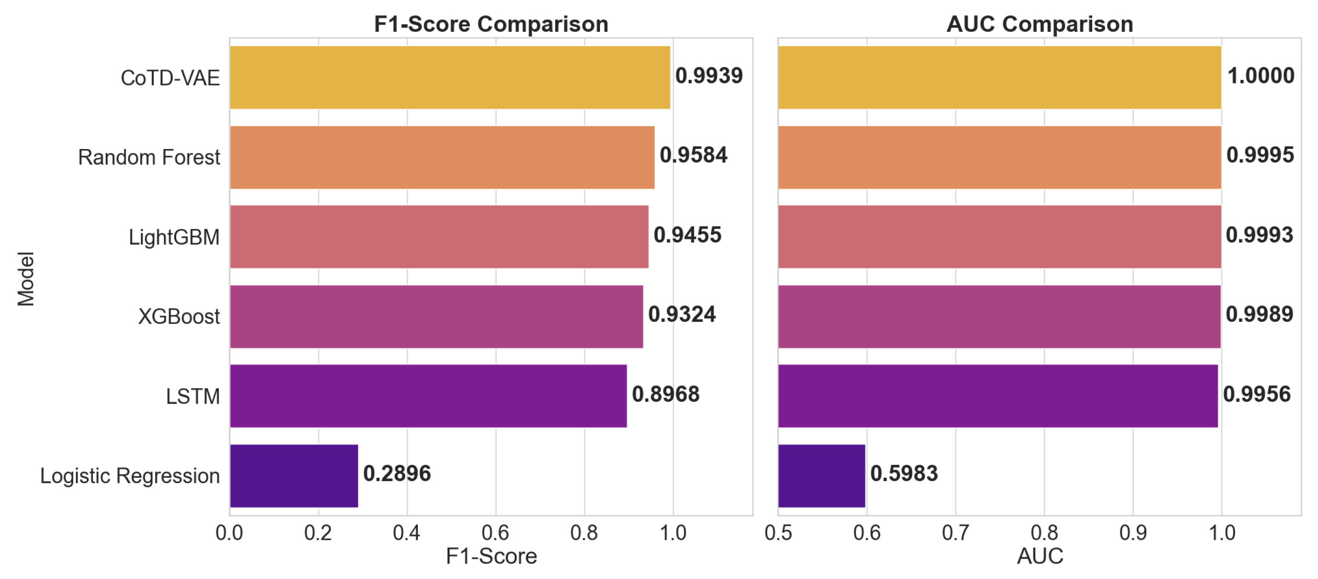
| CoTD-VAE | 0.9981 | 1.0000 | 0.9878 | 0.9939 | 1.0000 |
| Random Forest | 0.9863 | 0.9234 | 0.9961 | 0.9584 | 0.9995 |
| LightGBM | 0.9819 | 0.9008 | 0.9949 | 0.9455 | 0.9993 |
| XGBoost | 0.9773 | 0.8804 | 0.9910 | 0.9324 | 0.9989 |
| LSTM | 0.9641 | 0.8214 | 0.9875 | 0.8968 | 0.9956 |
| Logistic Regression | 0.6002 | 0.2013 | 0.5162 | 0.2896 | 0.5983 |
| Model | Accuracy | F1 Score | AUC |
|---|---|---|---|
| CoTD-VAE | 0.8707 | 0.6092 | 0.918 |
| No Smoothness | 0.8345 | 0.5588 | 0.912 |
| No Sparsity | 0.8248 | 0.5488 | 0.905 |
Disclaimer/Publisher’s Note: The statements, opinions and data contained in all publications are solely those of the individual author(s) and contributor(s) and not of MDPI and/or the editor(s). MDPI and/or the editor(s) disclaim responsibility for any injury to people or property resulting from any ideas, methods, instructions or products referred to in the content. |
© 2025 by the authors. Licensee MDPI, Basel, Switzerland. This article is an open access article distributed under the terms and conditions of the Creative Commons Attribution (CC BY) license (https://creativecommons.org/licenses/by/4.0/).
Share and Cite
Huang, L.; Chen, Q. CoTD-VAE: Interpretable Disentanglement of Static, Trend, and Event Components in Complex Time Series for Medical Applications. Appl. Sci. 2025, 15, 7975. https://doi.org/10.3390/app15147975
Huang L, Chen Q. CoTD-VAE: Interpretable Disentanglement of Static, Trend, and Event Components in Complex Time Series for Medical Applications. Applied Sciences. 2025; 15(14):7975. https://doi.org/10.3390/app15147975
Chicago/Turabian StyleHuang, Li, and Qingfeng Chen. 2025. "CoTD-VAE: Interpretable Disentanglement of Static, Trend, and Event Components in Complex Time Series for Medical Applications" Applied Sciences 15, no. 14: 7975. https://doi.org/10.3390/app15147975
APA StyleHuang, L., & Chen, Q. (2025). CoTD-VAE: Interpretable Disentanglement of Static, Trend, and Event Components in Complex Time Series for Medical Applications. Applied Sciences, 15(14), 7975. https://doi.org/10.3390/app15147975