Integrated Investigation of the Time Dynamics of Forest Fire Sequences in Basilicata Region (Southern Italy)

Abstract

The time fluctuations of forest fires occurring in Basilicata, a region situated in Southern Italy, between 2004 and 2023 were investigated using various analytical approaches. Analysis revealed a clustering of fire occurrences over time, as indicated by a significantly high coefficient of variation. This suggests that the fire sequence does not follow a Poisson distribution and instead exhibits a clustered structure, largely driven by the heightened frequency of events during the summer seasons. The analysis of monthly forest fire occurrences and total burned area indicates a significant correlation between the two. This correlation is reinforced by shared patterns, notably an annual cycle that appears to be influenced by meteorological factors, aligning with the yearly fluctuations in the region’s weather conditions typical of a Mediterranean climate. Furthermore, the relationship between the Standardized Precipitation Evapotranspiration Index (SPEI) and forest fires revealed that the accumulation period of the SPEI corresponds to the cycle length of the fires: longer cycles in fire occurrences align with higher accumulation periods in SPEI data.

1. Introduction

Forest fires could be considered as natural processes that play a crucial role in sustaining various life cycles and maintaining the biodiversity of numerous ecosystems [1]; however, they are undoubtedly perceived as destructive natural phenomena [2] causing land degradation [3], facilitating alien plant invasion and patch homogenization, and creating positive feedback mechanisms favoring fuel loading, and fire spreading and intensity [3,4]. Although fires have long been utilized as a manner of fertilizing soil and controlling plant growth, they can change vegetation, increase soil erosion, and are one of the factors causing desertification of previously fertile areas [5].

Investigating the time dynamics of fire sequences in a specific region is of great importance, since it could reveal features of fire dynamics linked with the meteo-climatic variability of that region or with the identification of the anthropogenic mechanisms of fire ignition. Thus, the application of robust methodologies allowing to extract features hidden in the complex time fluctuations of fire sequences is crucial. Telesca et al. [6] analyzed the fire sequence that occurred in Ticino (Switzerland) by using the Allan Factor method [7] revealing several features of fire dynamics like (1) the Poissonian behavior of the time distribution of the sequence at small timescales and the non-Poissonian character at larger timescales (or time clustering), suggesting the existence of “memory phenomena” in the time distribution of the fires; (2) the presence at low altitudes of two different fire regimes that tend to merge into one single fire regime at higher altitudes, suggesting the mixing of natural and anthropogenic mechanisms, with the predominance of natural-caused (lightning) fires at higher altitudes; (3) the existence of daily periodicities that respond to the diurnal weather changes, like the increase and decrease in temperature and solar radiation, influencing the daily fluctuation of the dead fuel moisture content of open woodland fuel [8,9]; and (4) the presence of the yearly cycle, which is the typical seasonal variability, as a result of the cumulative impact of weather and climate as well as vegetation, specifically, the litter and herb layer in the forest stand understory, which follows a seasonal growth cycle. Similar temporal patterns were found in other regions of southern Europe, such as Tuscany [10] and Portugal [11].

The temporal clustering of fires suggests a correlation among them: a fire in a previously unburned area creates a mosaic of burned and unburned vegetation patches, leading to feedback behavior that influences the likelihood of the occurrence of subsequent fires [12,13].

Although human-induced fires are dominant in most Mediterranean regions [14], the fuel amount and moisture that depend on climate variability govern the conditions of fire ignition and its characteristics [15], like its intensity, spread, and propagation that are also influenced by wind [16,17].

In the future, fires in Europe are expected to increase in number of events and intensity, and the climate has been recognized as one of the main drivers for future fire regimes [18,19]. In fact, projected climate scenarios indicate an increase in the duration and the severity of fire seasons due to the strengthening of warming and the increase in drought events for most southern European countries [20]. The fuel amount and moisture can be considered as the manifestation of the link between climate and fire [21,22,23]; in fact, fire spread is limited by fuel amount during high-drought periods, and by fuel moisture during low-drought periods, and both conditions play an important role in shaping fire regimes, especially in Mediterranean-type ecosystems [24]. The close link between climate and fires was analyzed in several works; in particular, it was suggested that drought conditions concomitantly with high temperatures could provoke the occurrence of larger fires [25,26,27,28,29,30]. However, climate can impact on fire activity across multiple timescales. For instance, Pausas (2004) [31] found that in southeastern Spain year-to-year variations were anticorrelated with concurrent summer rainfalls and positively correlated with summer rainfalls that occurred 2 years before. Similarly, significant correlation was revealed between forest fire activity and lagged climate variables in several southern European countries [17,26,30]. Turco et al. [32], using a large, high-quality database provided by the European Forest Fire Information System (EFFIS) [33], analyzed the impact of concomitant drought and previous wet conditions on the summer burned area in Mediterranean Europe by modeling the relationship between the Standardized Precipitation Evapotranspiration Index (SPEI) and the burned area; they found a statistically significant relationship between fire and same-summer droughts, while antecedent climate conditions appear to impact fire activity much less.

From the above, it is evident that forest fires represent a complex natural phenomenon that cannot be disentangled by other factors, like climate and weather, anthropogenic activities, and vegetation conditions [15].

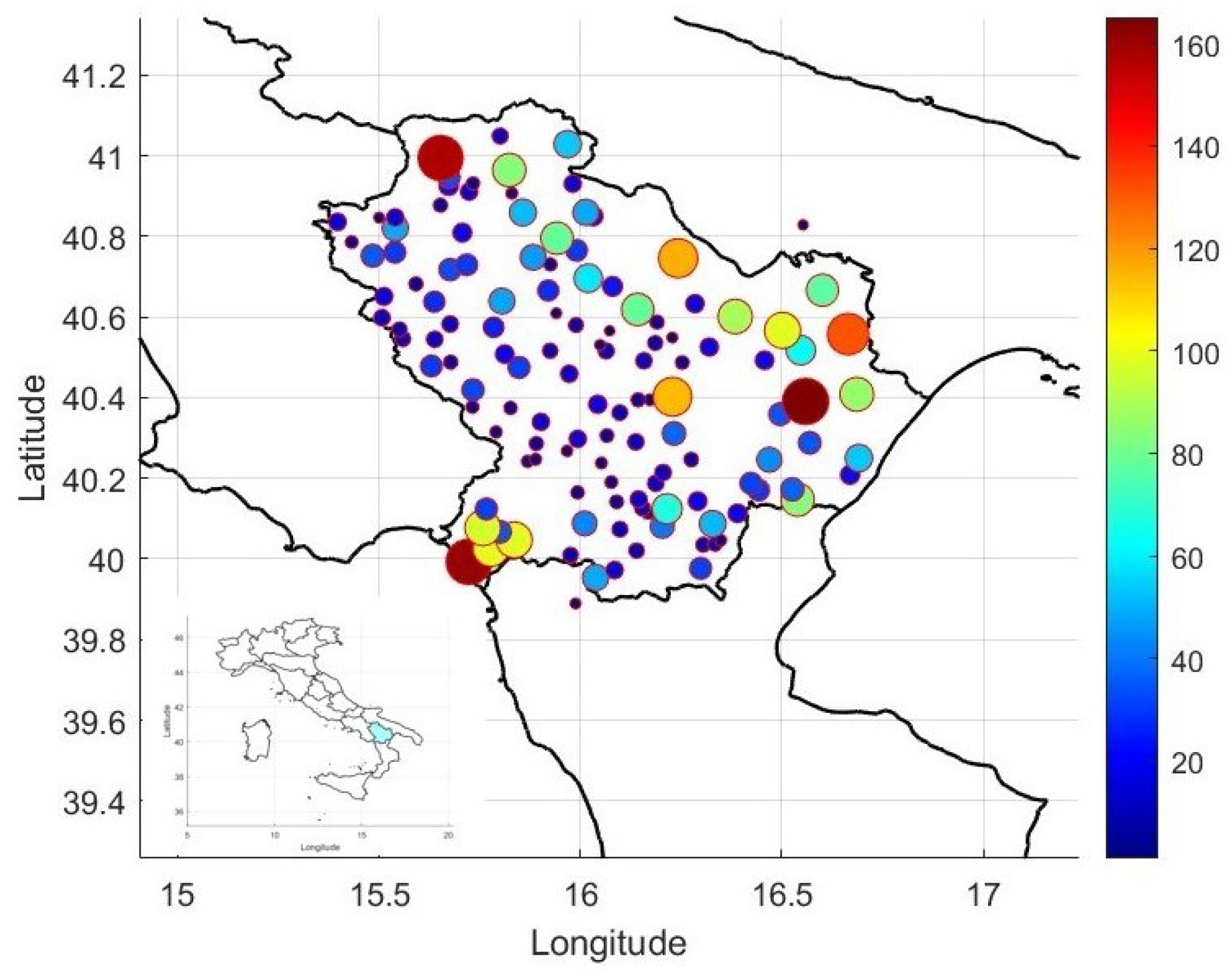
Forest fires, as a complex phenomenon, require advanced statistical methodologies to be thoroughly investigated from multiple perspectives. And in this context the objectives of this study are twofold: (1) To integrate different statistical approaches for the analysis of forest fire temporal dynamics, employing a combination of advanced techniques that, to our knowledge, have not been jointly applied in previous researches. While individual methods have been used in isolated cases, this study integrates them to explore the time dynamics of fire sequences and to investigate both short- and long-term relationships between fire activity and climatic variables, thereby offering a deeper and more holistic understanding of the underlying processes. (2) To conduct a high-resolution, localized analysis focused specifically on the Basilicata region (Southern Italy), representing the first study to investigate the temporal behavior of forest fires and their climatic drivers at fine spatial and temporal scales. Unlike most previous studies that analyze broader areas (e.g., entire countries or ecoregions) and rely on coarse temporal aggregations (e.g., annual or decadal), our study provides a detailed view capable of capturing fine-scale patterns and regional specificities.

This paper is organized as follows. Section 2 presents the study area, the forest fire dataset, and the Standardized Precipitation Evapotranspiration Index (SPEI), a well-known drought indicator. Section 3 outlines the statistical methods employed to investigate the fire sequence and its relationship with the SPEI. The results and a discussion of the main findings are provided in Section 4 and Section 5, respectively, while the conclusions are presented in Section 6.

2. Data

2.1. Study Area

The study area is the Basilicata region located in Southern Italy (Figure 1). The regional territory is about 10,000 km² mostly characterized by mountains (47%) and hills (45%) with a small flat percentage (8%). The climate is prevailing Mediterranean humid in the Apennine Mountain range and Mediterranean dry in the hilly and flat areas. The Regional Forest Atlas reports for the forest area of the Basilicata an extent of around 355,409 hectares, in full accordance with the National Inventory being drawn up by Forests and Carbon Reservoirs which attributes approximately 345,000 hectares of wooded area to the Basilicata region. Deciduous oak forests occupying 51.8% of the territory represent the majority of the forest cover, followed by beech forest (8.4%), Mediterranean macchia (7.9%), shrublands (6.9%), and other deciduous broad-leaved forests (5.5%); the remaining 19.5% are mainly made up of evergreen broad-leaved forests, Mediterranean pine forests, chestnut stands, hygrophilous forests, and garrigue. The rest of the territory is mainly devoted to agricultural activities.

2.2. Forest Fire Catalogue

The catalogue of forest fires is freely available at https://rsdi.regione.basilicata.it/ (accessed on 20 March 2025). For each fire event, the catalogue reports the date of occurrence, the location, and the extent of the burned area, along with other information. The fire data were pre-processed to produce the interevent times (i.e., the time interval between two consecutive fire events in days) and the monthly number of fires and monthly total burned area.

2.3. The Standardized Precipitation Evapotranspiration Index

The Standardized Precipitation Evapotranspiration Index (SPEI) is an index used to estimate drought intensity. The SPEI relies on a monthly climatic water balance, which involves subtracting potential evapotranspiration from precipitation. Details of the calculation of the SPEI can be found in [34]. If the SPEI is positive, this indicates above-normal wet conditions, while if it negative, this identifies dry situations.

The SPEI was obtained from http://sac.csic.es/spei/database.html (accessed on 20 March 2025), which contains data at the global scale, with a 0.5 degrees spatial resolution and a monthly time resolution. The SPEI is provided with accumulation times ($T_a$) ranging from 1 to 48 months starting in January 1901.

For our purposes, we extracted the SPEI for $T_a$ from 1 to 48 months at location (40.25°, 16.25°), which is included in the investigated area. The extracted SPEI_B from May 2004 to November 2018 (that is the period of investigation of the fire sequence) is representative of the climatic (wet/dry) conditions of the area under study. Figure 2 shows the time variation of SPEI_B for some typical $T_a$.

3. Methods

A fire sequence of N events can be represented as a temporal point process $x\left(t\right)$ marked by the burned area A

$$x\left(t\right)=\sum _i^N{A}_i\delta (t-t_i)$$

(1)

where $t_i$ is the time of occurrence of the fire i with burned area $A_i$ and $\delta \left(t\right)$ is the Dirac’s delta function that is zero for all t except $t_i$.

After choosing a specific time window, such as one month or one year, an alternative representation of the fire occurrence is the time series depicting the count of fires or the cumulative burned area within that window.

3.1. The Coefficient of Variation

The coefficient of variation $C_v$ [35] is a simple quantity used to investigate the time structure of a sequence; in particular, it allows to discern if the sequence is periodic or quasi-periodic, purely random, or time-clusterized. A periodic or quasi-periodic sequence is characterized by events that occur regularly or almost regularly on time. In a purely random sequence, the events occur randomly on time, like a Poisson process; in this case the events occur homogeneously in time and the occurrence rate is almost constant. In a time-clusterized sequence, the events occur in clusters and not homogeneously; thus, the frequency of event occurrence changes with the time. The coefficient of variation is defined as

$$C_v={\displaystyle \frac{{\widehat{\sigma }}_T}{{\widehat{\mu }}_T}}$$

(2)

where ${\widehat{\sigma }}_T$ is the standard deviation and ${\widehat{\mu }}_T$ is the average of the set of time intervals between two consecutive fire events $\{T_i,i=1,\dots ,N\}$ known as interevent intervals.

For a Poissonian sequence $C_v$ is 1. If the set of events is governed by cyclic or quasi-periodic dynamics, $C_v<1$. If the sequence is time-clustered, $C_v>1$. The 95% confidence interval of the estimate of $C_v$ can be calculated by generating a huge number of surrogate Poissonian sequences with the same number of events and same mean interevent time of the original one.

It should be emphasized that while a Poisson process implies a $C_v$ equal to 1, the converse is not necessarily true; that is, a $C_v$ of 1 does not necessarily imply that the process is Poissonian. The coefficient of variation can be considered a global measure of the time structure of a sequence.

3.2. The Allan Factor

The Allan Factor (AF) is a tool commonly employed to analyze the temporal dynamics of various natural phenomena [36]. Compared to the coefficient of variation ($C_v$), it provides a more refined assessment of the temporal structure within a sequence. While $C_v$ can distinguish between Poissonian, clustered, or regular event patterns, the AF additionally identifies the specific temporal scales at which these behaviors occur. To compute the AF, the time axis is partitioned into contiguous, equally sized intervals of duration $\tau$, referred to as the timescale. Within each interval, the number of events is counted, yielding a sequence $\left\{N_k\left(\tau \right)\right\}$ where $N_k$ denotes the number of events falling in the k-th window [37]. The Allan Factor is then defined by the following formula:

$$AF\left(\tau \right)={\displaystyle \frac{<{(N_{k+1}\left(\tau \right)-N_k\left(\tau \right))}^2>}{2<N_k\left(\tau \right)>}}$$

(3)

where $<..>$ indicates the average value. A Poissonian sequence, whose events are uncorrelated and independent, is characterized by the AF being rather flat for all the investigated timescales assuming a value around 1, except for very large timescales due to finite-size effects [38]. A decrease in the AF at a specific timescale indicates that the sequence exhibits periodic behavior at that scale [39]. Conversely, a time-clustered sequence is characterized by a scale-dependent AF; in particular, for a fractal (self-similar) process, the AF increases with the timescale $\tau$ following a power-law relationship:

$$AF\left(\tau \right)\approx {\tau }^{\alpha }.$$

(4)

A power-law behavior of the AF indicates that the sequence is characterized by correlation among the events [37]. The exponent $\alpha$ is called the fractal exponent and quantifies the intensity of the time clusterization or time correlation. Thus, if the null hypothesis $\alpha =0$ is not rejected against the alternative hypothesis $\alpha >0$, the sequence of interevent intervals $\left(T_i\right)$ is assumed to follow a Poissonian behavior. Conversely, if there is sufficient evidence to reject the null hypothesis $\alpha =0$, the sequence $\left(T_i\right)$ is assumed to exhibit a time-clustered pattern.

In order to investigate the significance of the AF, random sequences can be generated with two surrogate methods: (1) the Poissonian surrogate method, consisting of generating Poisson-distributed sequences with the same rate as the original one; and (2) the random permutating method [40], consisting of generating random shuffles of the interevent times of the original sequence; with the second surrogate method, the distribution of the original interevent times does not change. After calculating the AF for each surrogate, the distribution of AF values for each timescale $\tau$ is computed. For instance, by setting a confidence level of 97.5%, the 97.5% confidence curve corresponds to the envelope of all 97.5th percentiles. If the AF is significantly above the Poissonian confidence level, it indicates a notable deviation from Poissonian behavior. Similarly, if it is well above the confidence curve derived from random shuffles of interevent times, this suggests that the clustering behavior is not driven by the probability density of interevent times.

3.3. The Schuster’s Spectrum

The Schuster test has been used to investigate periodic patterns in natural point processes [41]. Assuming that the probability of event occurrences follows a sinusoidal function with period T, each occurrence time $t_k$ of the k-th event can be associated with a phase ${\theta }_k={\displaystyle \frac{2\pi t_k}{T}}$. This transforms the sequence of N occurrence times into a two-dimensional unit-length random walk, where each step changes direction according to the phase ${\theta }_k$.

Let D be the distance between the starting point and the endpoint of this walk. The probability p of obtaining a distance greater than or equal to D under the null hypothesis of uniformly distributed occurrence times corresponds to the probability that such a pattern could arise by chance. This probability is referred to as Schuster’s p-value, and it is given by:

$$p=e^{-{\displaystyle \frac{D^2}{N}}}.$$

(5)

Therefore, the likelihood of a periodicity at period T increases as the Schuster’s p-value decreases. The number M of Schuster’s tests performed is given by [42]

$$M={\displaystyle \frac{t}{ϵ}}\left({\displaystyle \frac{1}{T_{min}}}-{\displaystyle \frac{1}{T_{max}}}\right).$$

(6)

where $T_{min}$ and $T_{max}$ are, respectively, the minimum and the maximum of the periods to be tested, and $ϵ$ is usually 1.

As demonstrated in [42], if the Schuster p-value of a periodicity T is significantly lower than $T/t$, then T can be considered to be not due to chance.

3.4. The Correlogram-Based Periodogram

The power spectrum of a time series represents the frequency distribution of series’ power at different frequency bands. It is commonly employed to discern cyclic patterns within time series data, as manifested by peaks in the power spectrum corresponding to the periods of these cycles. In the case of purely random processes, such as white noise, the power spectrum remains approximately constant across all frequencies; this signifies that the series is entirely uncorrelated, with each value being completely independent of the others.

In this study, since the time series we will analyze are short, we will employ the correlogram-based periodogram, which has proven to be an efficient method for estimating the power spectrum of short time series with only a few dozen samples [43].

The simple model of periodic series is:

$$y_n=\beta cos(\omega t+\varphi )+{ϵ}_n$$

(7)

with $\beta >0$, $0<\omega <\pi$, $\varphi$ distributed as a uniform random variable in $(-\pi ,\pi ]$, and $\left\{{ϵ}_n\right\}$ denoting a sequence of uncorrelated random variables with zero mean and standard deviation $\sigma$, independent of $\varphi$.

The classical periodogram is given by

$$I\left(\omega \right)={\displaystyle \frac{1}{N}}|\sum _{n=1}^N{y}_n{e}^{-i\omega n}{|}^2,0\le \omega \le \pi$$

(8)

with N being the length of the series, and it is calculated for

$${\omega }_l={\displaystyle \frac{2\pi l}{N}}, l=0,1,\dots ,a$$

(9)

where $a=\left[{\displaystyle \frac{N-1}{2}}\right]$ and $\left[x\right]$ indicates the integer part of x. If a strong cycle with frequency ${\omega }_0$ modulates the series, the periodogram peaks at ${\omega }_0$, while, if the series is uncorrelated $(\beta =0)$, according to Priestley [44], the classical periodogram is uniformly distributed across the frequencies. To improve the detection of periodic components in a time series, Ahdesmäki et al. [43] introduced the correlogram-based periodogram, which has been shown to be a more effective tool for identifying cyclic patterns compared to the traditional approach. The periodogram $I\left(\omega \right)$ is equivalent to the correlogram:

$$S\left(\omega \right)=\sum _{k=-N+1}^{N-1}\widehat{r}\left(k\right)e^{-i\omega k}$$

(10)

where

$$\widehat{r}\left(m\right)={\displaystyle \frac{1}{N}}\sum _{k=1}^{N-m}{y}_k{y}_{k+m}$$

(11)

estimates the autocorrelation function. By using the sample autocorrelation function

$$\rho \left(m\right)={\displaystyle \frac{\frac{1}{N}{\sum }_{i=1}^N(x_i-\overline{x})(y_i-\overline{y})}{{\sigma }_x{\sigma }_y}}$$

(12)

where $\overline{x}$ indicates the mean, the correlogram-based periodogram proposed by Ahdesmäki et al. [43] for estimating the power spectral density of a series is the following:

$$\tilde{S}\left(\omega \right)=2Re\left(\sum _{k=0}^L\tilde{\rho }\left(k\right)e^{-i\omega k}\right)-\tilde{\rho }\left(0\right).$$

(13)

where the real part of x is indicated by $Re\left(x\right)$, the series’ length by N, and the biased Spearman rank correlation coefficient by $\tilde{\rho }\left(m\right)$. If the classical periodogram is always positive, the correlogram-based periodogram could be negative; therefore, the absolute value is taken.

To test the significance of a frequency ${\omega }_l$, the g-statistics could be used:

$$g={\displaystyle \frac{\left|\tilde{S}\left({\omega }_l\right)\right|}{{\sum }_{i=1}^a\left|\tilde{S}\left({\omega }_i\right)\right|}}.$$

(14)

A large value of g at a specific frequency indicates that this frequency carries substantial power in the signal, suggesting it is statistically significant. The statistical significance of a tested frequency can be evaluated using a simulation-based approach [43]. Specifically, by employing Equation (7), we generate a set of random time series, and for each simulated series, the corresponding g-value is computed using Equation (14). The collection of these g-values is then used to approximate the distribution of the g-statistic, from which the associated p-value is estimated. A low p-value indicates a strong presence of the tested frequency in the original series.

3.5. Empirical Mode Decomposition

The Empirical Mode Decomposition (EMD), introduced by Huang et al. [45], is a method designed to decompose a time series $x\left(t\right)$ into a set of components known as Intrinsic Mode Functions (IMFs). These IMFs must fulfill two criteria: (1) the count of local extrema and zero-crossings can differ by no more than one; and (2) at every point in time, the mean of the upper and lower envelopes—constructed from the local maxima and minima, respectively—is zero. While Empirical Mode Decomposition (EMD) was adopted in this study due to its adaptive and data-driven nature, it is worth noting that other signal decomposition techniques, such as the Wavelet Transform (WT) [46] and Singular Spectrum Analysis (SSA) [47], are also commonly employed. EMD offers the advantage of not requiring a priori selection of basis functions or decomposition levels (as in WT), or the number of components (as in SSA), making it particularly suitable for non-linear and non-stationary time series such as those analyzed in this work.

To decompose a series into the IMFs, the following sifting algorithm is employed [48]:

• Detect all minima and maxima points of the original signal $x\left(t\right)$.
• Form the lower envelope $E_{\mathrm{lower}}\left(t\right)$ and upper envelope $E_{\mathrm{upper}}\left(t\right)$ by using the cubic spline interpolation technique for minima and maxima data points.
• Calculate the mean envelope $E_{\mathrm{mean}}\left(t\right)={\displaystyle \frac{E_{\mathrm{lower}}\left(t\right)+E_{\mathrm{upper}}\left(t\right)}{2}}$.
• Compute the signal $s\left(t\right)=x\left(t\right)-E_{\mathrm{mean}}\left(t\right)$.
• Verify the two conditions for $s\left(t\right)$ to determine if it qualifies to be an IMF.
• If $s\left(t\right)$ qualifies to be an IMF, then set ${\mathrm{IMF}}_n\left(t\right)=s\left(t\right)$ and repeat the procedure from step (1) for the residual signal $\mathrm{res}\left(t\right)=x\left(t\right)-s\left(t\right)$; otherwise, replace $x\left(t\right)$ with $s\left(t\right)$ and repeat the procedure.
• Repeat steps (1) to (6) until a monotonic residual signal $\mathrm{res}\left(t\right)$ is obtained.

4. Results

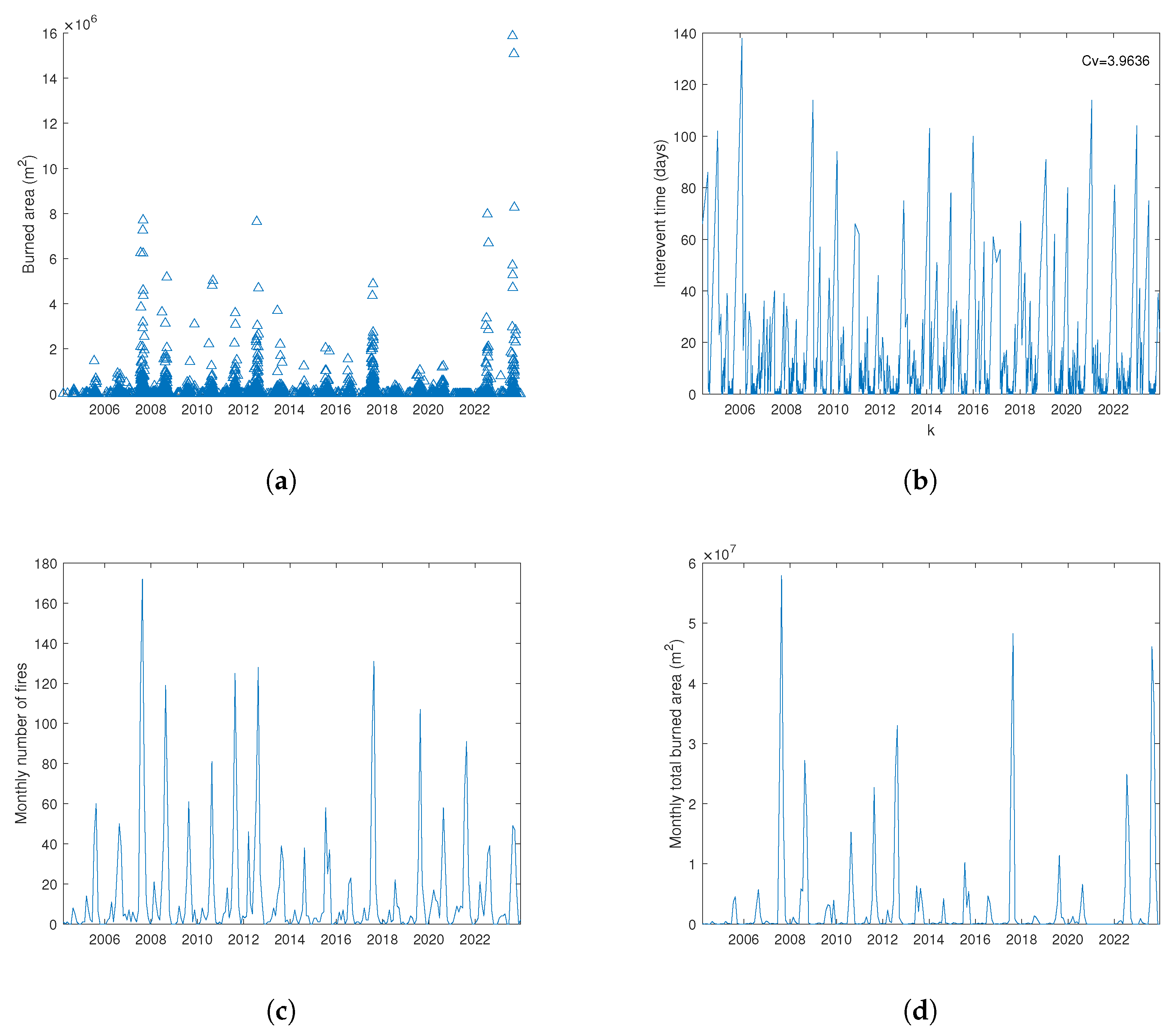
We analyzed the sequence of fires that occurred in the Basilicata region (Southern Italy) from 2004 to 2023 (Figure 3a).

Considering the series of the interevent times (Figure 3b), we found $C_v=3.96$. To calculate the 95% confidence interval of this estimate, a total of 1000 Poisson surrogate fire sequences were generated, each having the same number of fires and the same mean interevent time as the original series. The resulting 95% confidence interval for $C_v$ is given by $\left[0.96,1.03\right]$, where the lower and upper bounds correspond to the 2.5th and 97.5th percentiles, respectively, of the $C_v$ distribution obtained from the Poissonian surrogate sequences. As can be seen, the fire series is highly time-clusterized at a global scale, being $C_v$ well beyond the 95% confidence interval. The time clustering of the fire sequence is rather high due to the temporal occurrence pattern of fire events, which is much denser during the summer months; therefore, considering the entire sequence, there is an increase in frequency during the summer, structuring the entire sequence as composed of a set of clusters.

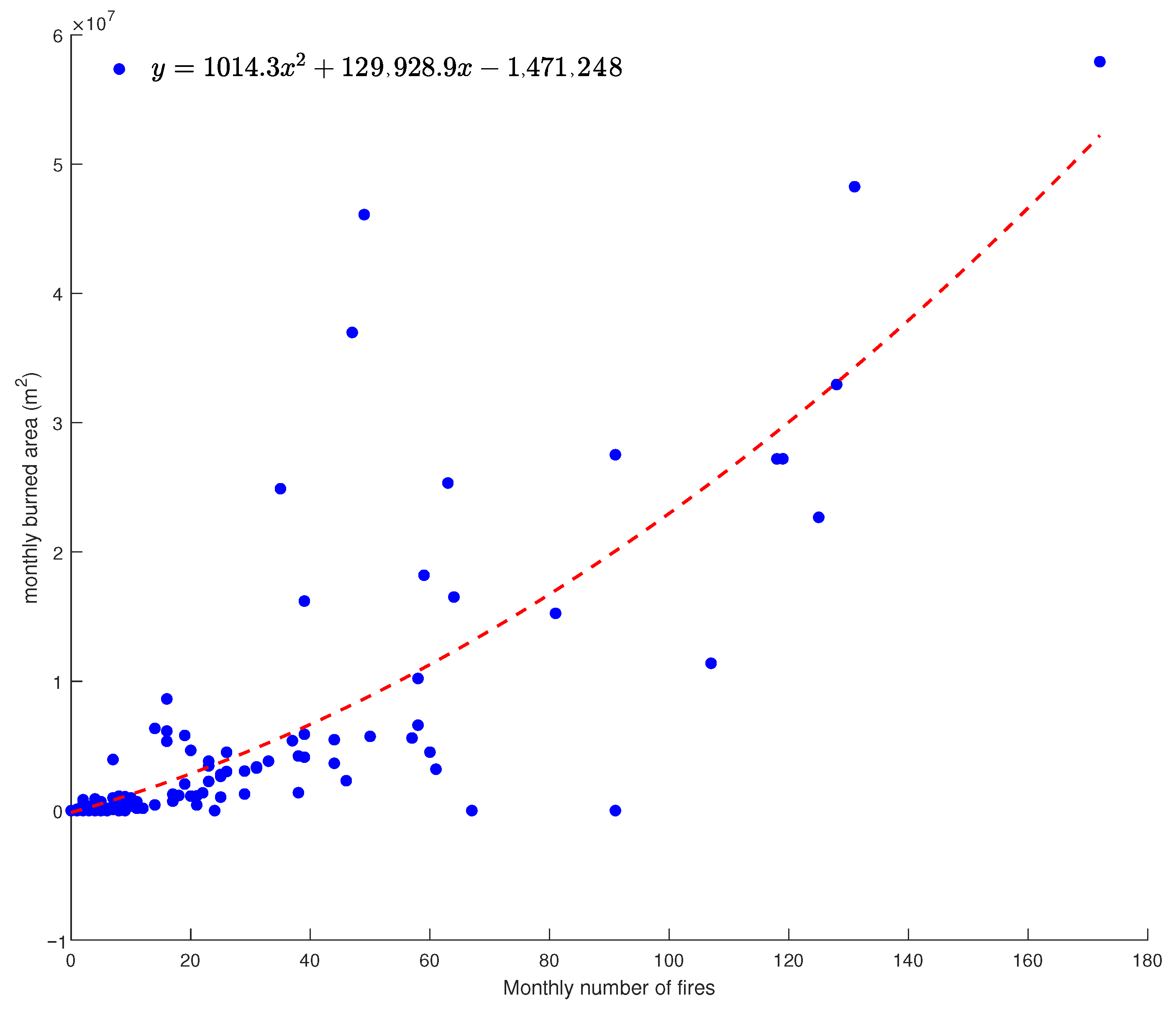
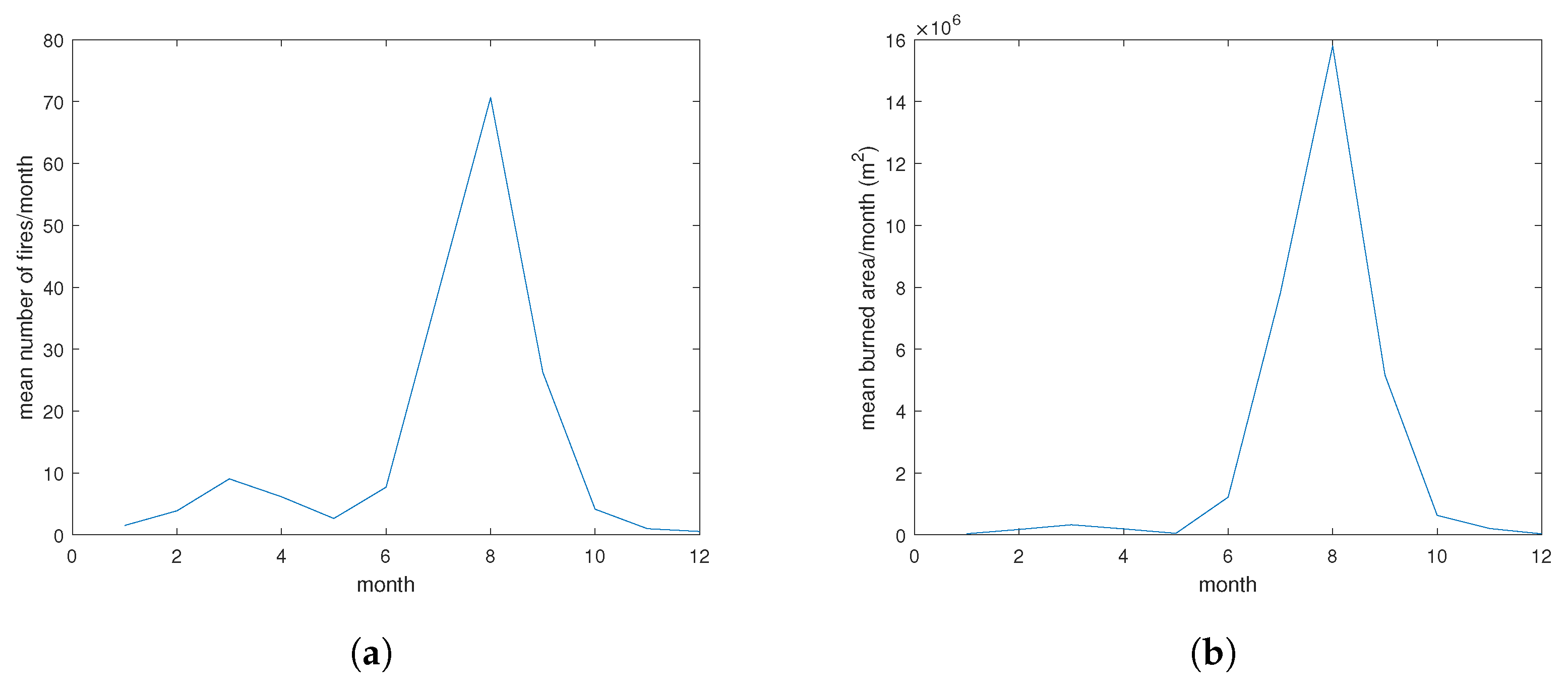
Figure 3c,d display the monthly number of fires and the monthly total burned area, respectively; the two variables are very similar, as confirmed by the relationship between them (Figure 4).

Figure 5a shows the AF for the analyzed fire sequence and the 97.5% confidence level calculated for 100 random sequences obtained with the Poissonian surrogate method and the random permutating method. The confidence envelopes were constructed from the pointwise 97.5th percentiles of the surrogate ensemble. No additional smoothing was applied to the confidence bands, in order to preserve their natural variability and accurately reflect the statistical variability across timescales. The AF of the original sequence of fires increases with $\tau$, indicating that the sequence is clusterized in time. The AF is well above the confidence curve obtained by Poissonian surrogates, suggesting that its non-Poissonian character is significant for all the investigated timescales. The AF falls below the confidence level for the random shuffles of interevent times up to approximately one week; this suggests that the clustering behavior is influenced by the probability density of interevent times within this shorter timescale range. Conversely, for longer timescales, the clustering behavior depends on the ordering of interevent times. At the 1-year timescale, the AF exhibits a drop, indicating the presence of annual periodic fluctuations in the fire sequence. Between about 2 weeks and 3 months, we can identify a fractal behavior, revealed by the power-law increase of the AF with $\tau$; within this timescale range the fractal exponent $\alpha \sim 1.4$, which indicates that the fire series is characterized by correlation among the events.

Figure 5b displays the Schuster spectrum. For each tested period, ranging from 1 day up to half the total duration of the observation period, the corresponding p-value (represented by circles) was computed. Several periods exhibit p-values below the 99% confidence threshold (indicated by the red line). Notably, periods of approximately 3 months and 1 year stand out as having the lowest p-values, indicating a strong periodic component at these timescales. The yearly period is in agreement with the annual timescale identified in the previous AF analysis, signaling the presence of the 1-year periodicity in the time dynamics of the fires. In addition, a period of about 5 years is revealed in Schuster’s spectrum.

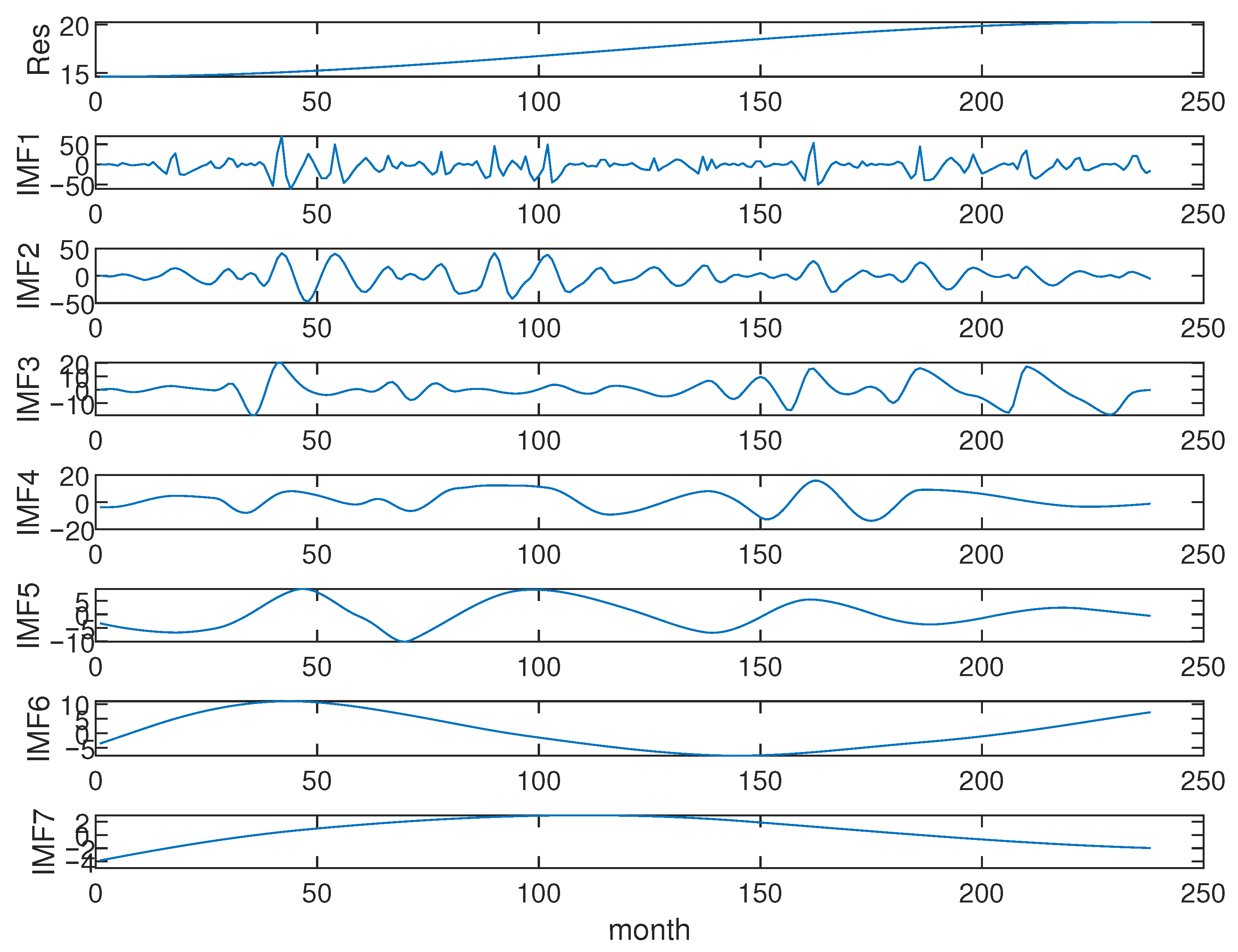
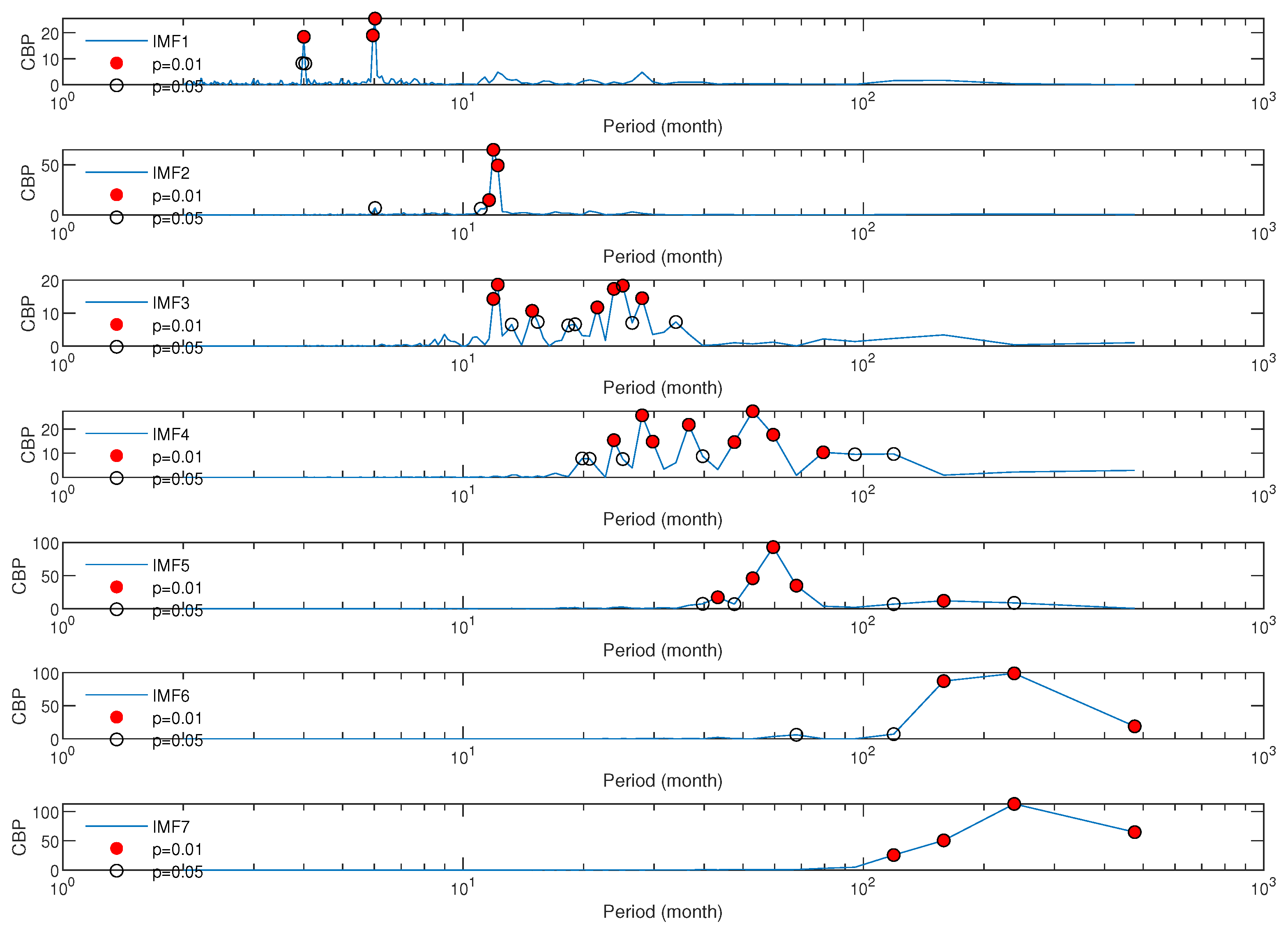
We applied the EMD analysis to the monthly number of fires and the monthly total burned area. Figure 6 shows results of the EMD of the monthly counts, while Figure 7 shows the correlogram-based periodogram (CBP) of the IMFs. The CBP’s evidence period is significant at 95% (hollow circles) and at 99% (red circles). Among the peaks significant at 99%, the highest ones signal the characteristic modulating frequencies of the IMFs. IMF₁ exhibits periodicities of 4 months and 6 months; IMF₂ is marked by an annual periodicity, while IMF₃ shows periodicities of about 12 months and 25 months; IMF₄ is marked by periods of 28, 36 and 53 months, while IMF₅ by a cycle of 60 months. IMF₆ and IMF₇ represent the long-term components of the monthly counts, since they are modulated by periods corresponding approximately to the length of the series.

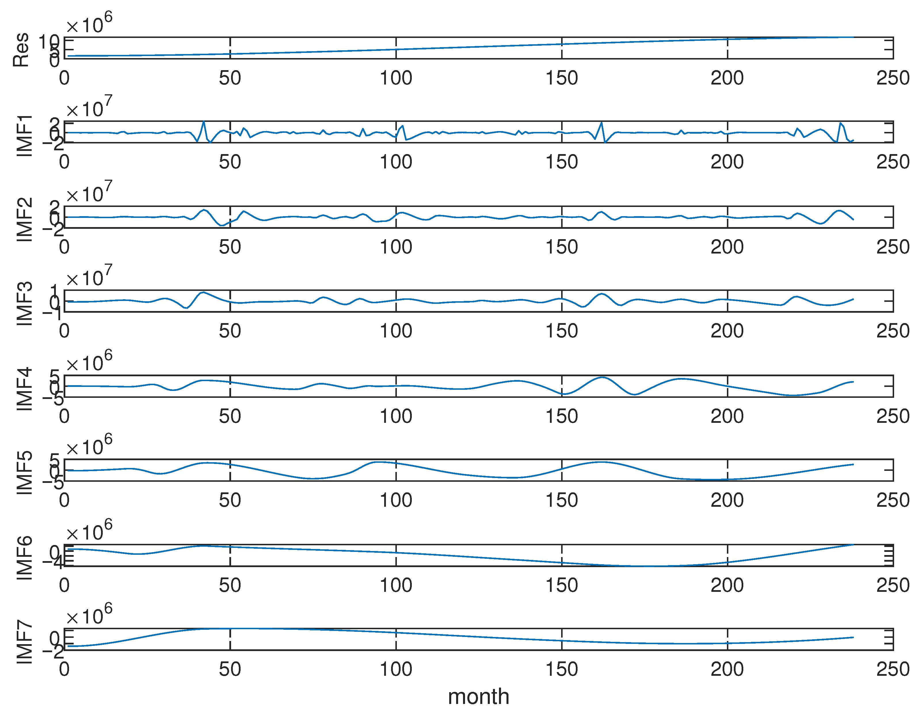
Figure 8 shows the results of the EMD of the monthly total area, and Figure 9 shows the CBP of the IMFs. The first two IMFs are characterized by the same modulating frequencies as the first two IMFs in the monthly counts. The third IMF shows only one main characteristic periodicity at 12 months. The fourth IMF is mainly modulated by 26-month and 48-month periodicities, while the fifth one mainly by a 60-month periodicity. IMF₆ and IMF₇ represent the long-term components of the monthly burned area as for the monthly counts.

Table 1. Main periodicities of the IMFs of the monthly number of fires and monthly burned area (the highest ones are bolded).

	Monthly Number	Monthly BA
IMF1	4 months, 6 months	4 months, 6 months
IMF2	1 year	1 year
IMF3	1 year, ≈25 months	1 year
IMF4	28 months, ≈3 years, 53 months	≈26 months, ≈ 4 years
IMF5	≈5 years	≈5 years
IMF6	≈20 years	≈20 years
IMF7	≈20 years	≈20 years

shows the main periodicities for each IMF of the monthly number and burned area series (the highest one is in bold).

The monthly counts and the monthly total burned area unveil various components: intra-annual, with the main modulating periods at 4 and 6 months; annual; quasi-bi-annual; intermediate-term, with the main modulating periods from about 3 to 5 years; and long-term, with the main modulating periods at about 20 years.

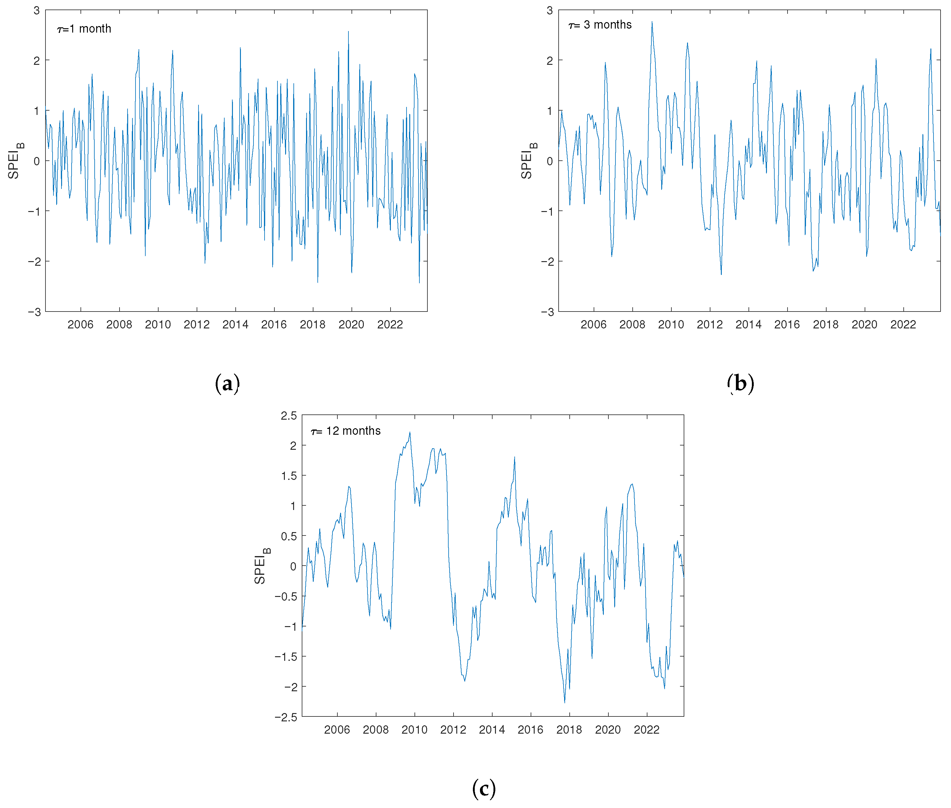
We explored the relationship between SPEI_B (calculated for the Basilicata region) and the IMF components of monthly counts and total burned area derived from EMD. Pearson’s correlation coefficient $\rho$ was computed between each ${\mathrm{SPEI}}_B\left(T_a\right)$ for $T_a=1,\dots ,48$ and each IMF. The left panels of Figure 10 and Figure 11 illustrate the correlation coefficient $\rho$ as a function of $T_a$ for the monthly counts and monthly total burned area, respectively. At the top of each plot in the left panel, the maximum $\left|\rho \right|$, its p-value, and the corresponding accumulation time $T_{a,max}$ are displayed. The right panels of Figure 10 and Figure 11 exhibit the comparison between the SPEI_B at $T_{a,max}$ alongside the corresponding IMF. Taking into account only the correlation coefficients with a p-value less than 0.05, the $T_{a,max}$ of SPEI_B that exhibit correlations with the IMFs of the monthly counts are 1, 3, 10, 30, 36, and 48 months. 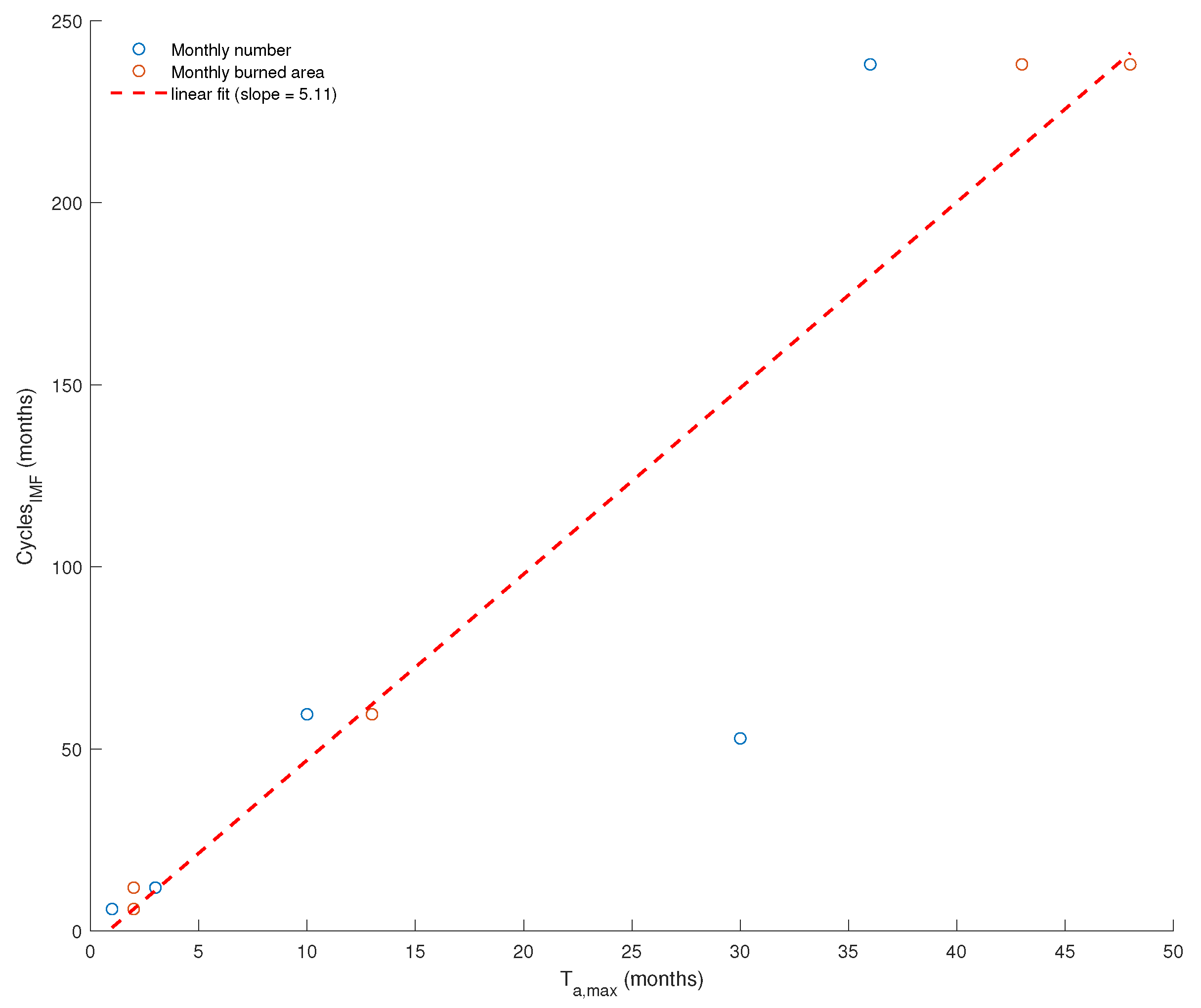Similarly, the significant timescales of SPEI_B that show correlations with the IMFs of the monthly total burned area are 2, 13, 43, and 48 months.

Table 2. Results of correlation analysis between SPEI_B and the IMF of the monthly number of fires.

${\mathit{T}}_{\mathit{a},\mathit{max}}$ (SPEIB)	IMF	$\mathit{\rho }$
1 month	IMF1	−0.18
3 months	IMF2	−0.19
10 months	IMF5	−0.51
30 months	IMF4	0.34
36 months	IMF6	0.21
48 months	IMF7	0.70

and

Table 3. Results of correlation analysis between SPEI_B and the IMF of the monthly total burned area.

${\mathit{T}}_{\mathit{a},\mathit{max}}$ (SPEIB)	IMF	$\mathit{\rho }$
2 months	IMF1	−0.13
2 months	IMF2	−0.11
13 months	IMF5	0.46
43 months	IMF6	0.34
48 months	IMF7	0.73

summarize the results of the correlation analysis between SPEI_B and IMFs of the monthly number of fires and total burned area, respectively.

5. Discussion

This study was conducted to explore the time dynamics of the sequence of forest fires recorded in Basilicata (Southern Italy). The occurrence of forest fires can be modeled as a stochastic point process, where each event is defined by its time of occurrence and the extent of the burned area. By employing various representations of the fire process, including interevent times and count series, alongside several statistical measures, we examined the fire regimes in the investigated sequence.

5.1. Time-Clustering

The fire activity exhibits time-clusterized or non-Poissonian behavior, as evidenced by the coefficient of variation $C_V$ significantly larger than 1, and by the non-flat behavior of the AF curve across all timescales. This finding suggests the existence of time-clustered behavior within the dynamics of fires, indicating correlated structures in the temporal distribution of fire events. For timescales shorter than ≈2 weeks, the time-clustering is influenced by the probability density function of the interevent times. This suggests that the time dynamics of fires is primarily determined by the distribution of short and long intervals between consecutive fires. On larger timescales, the time-clustering depends upon the ordering of interevent times. This implies that the temporal structure of events is primarily shaped by the specific succession of fires. In particular, between ≈2 weeks (${\tau }_1$) and 3 months (${\tau }_2$), the time-clustering of the fire activity is characterized by a scaling behavior (power law in log-log scales) with scaling exponent $\alpha \approx 1.4$ that indicates the existence of a fractal or self-similar structure in the time distribution of the fire events. The fractal structure is very common in many natural phenomena, and thus, it could be reasonably considered a natural behavior of the fire time dynamics. The fractal nature of fire activity across timescales ranging from a few days to a few months indicates that fire occurrences exhibit a consistent temporal structure that remains unchanged regardless of the scale considered; in other words, the time distribution of fire events remains nearly constant as we move from larger to smaller timescales.

If a scaling exponent $\alpha \approx$ 0 indicates that the process is Poissonian, and thus characterized by independent and uncorrelated events, a value of $\alpha \approx$ 1.4 suggests a rather high degree of clusterization and correlation among the fire events. In a joint analysis of wildfire occurrences and weather conditions in Japan, Ref. [49] discovered that there is a significant likelihood of fire occurrence when the average humidity drops below 60%, indicating a strong correlation between fire events and climate; and Ref. [50] in their analysis of the temporal clustering of humidity events (identified by instances when humidity drops below 60%), discovered that the temporal clustering of the humidity process exhibits fractal behavior with an exponent approximately equal to 1.07, in agreement with that of Japanese wildfires.

The found fractal behavior of our fire dataset agrees with that discovered in other fire sequences, and it is very likely that its behavior might be induced by similar meteo-climatic patterns.

5.2. Characteristic Timescales

The timescale ${\tau }_1\approx 2$ weeks is consistent with the findings of [6,50] focused on fire activities that occurred in several areas of the world, and could have an anthropic origin [50]; indeed, activities related, for instance, to agriculture, such as burning stubble during the summer months, might be scheduled on a quasi-weekly basis and this could have an effect by exerting the quasi-weekly timescale. Ref. [51] used statistical methodologies well suited for detecting weekly periodicities in time series of fire counts and for identifying the weekday with the lowest number of fires; their study revealed how the anthropogenic activity impacts on the seasonal character of global vegetation burning, by precisely individuating a global fire activity cycle with a minimum on weekends. Such a minimum was presumably due to labor laws in most countries and the influence of the Christian religion that prescribes Sunday as the weekday of rest. However, it cannot be excluded that weekly meteo-climatic factors could affect fuel moisture in a site-specific way [52].

The increased occurrence of fires during the summer months might lead to the emergence of the timescale ${\tau }_2\approx 3$ months, representing the upper timescale of the fractal regime in the time distribution of fire events, but also linked with the seasonality of the meteo-climatic conditions of the investigated area. Until a timescale of about 3 months, fire events exhibit consistent scaling properties, likely driven by similar meteo-climatic conditions. However, beyond ${\tau }_2$, there may occur a blending of various temporal dynamics influenced by different meteo-climatic conditions, causing the time distribution of fires to deviate from fractal behavior, as evidenced by the lack of scaling observed in the AF curve for timescales larger than ${\tau }_2$.

5.3. Cycles

The annual cycle stands out as the most apparent periodicity in the analyzed fire sequence, evidenced by the drop in the AF curve occurring approximately over a one-year timescale. This is also reflected in Schuster’s spectrum, where the most significant period (corresponding to the lowest p-value) aligns with one year. The annual cycle is also discernible in the second IMF of the EMD applied to the monthly fire number and the monthly total burned area. The nature of the yearly cycle is undoubtedly meteorological, as it mirrors the annual periodicity of the meteorological and climatic conditions in the investigated area, characterized by a Mediterranean climate that follows a yearly cycle.

Both the monthly number of fires and the total burned area exhibit a similar average annual bell-shaped pattern: fires are at their lowest in winter, gradually increase in spring, peak in summer, and then decrease in autumn (Figure 12). The striking similarity between the two patterns confirms a high correlation between the number of fires and the burned area, as illustrated in Figure 4. Forest fires are primarily influenced by factors such as relatively high temperatures and human activities related to land management, like the burning of stubble after harvesting crops. These factors typically reach their peak during the summer months, particularly in August.

In addition to the annual cycle, the other cycles identified in the IMFs (i.e., sub-annual, interannual, and decadal) can also be considered as induced by the meteo-climatic seasonality of the investigated area.

5.4. Relationship Between Fires and SPEI

The inter-relationship between fires and climate has always been a subject of paramount importance in the scientific context devoted to fires. While fires undoubtedly affect climate change, climatic factors, like rainfall and temperature, not only directly impact the probability of fires but can also indirectly alter vegetation productivity (i.e., fuel abundance), consequently affecting the intensity of fires [53,54,55]. In regions abundant with biomass, the primary factors driving wildfire activity are typically high temperatures and seasonal drought conditions [56,57]. Extreme and prolonged droughts, induced by abnormal fluctuations in the climate system like El Niño, have consistently served as significant catalysts for regional fires [54,58]. On a global scale, greater seasonal variation with summer and autumn being the seasons with the most frequent fire occurrence worldwide was found by using satellite data and investigating the spatial distribution, intensity, emission changes, and meteorological differences between fires in different fire-active and fire-prone regions [59].

The SPEI is a well-known drought driver and its link with fires was demonstrated in several studies. For instance, it was statistically shown that same-summer-drought conditions play a dominant role for fires in Mediterranean Europe [26]; in particular, the correlation between burned area and coincident SPEI3 (i.e., calculated for an accumulation period $T_a$ = 3 months) for July and August (when usually the temperature reaches its highest value) is large in all the Mediterranean ecosystems that are characterized by a relatively high abundance of fine fuels able to dry out quickly during a single summer [32]. A correlation analysis between the SPEI (decomposed in trend and season through the LOESS method [60]) and fires in inland areas of Spain showed that short-term droughts (SPEI3 and SPEI6) have a more significant impact on fire occurrence than prolonged droughts (SPEI12 and SPEI24), while the seasonal cycles of burned area seem to be strongly associated to SPEI24, thus with prolonged dry conditions [61].

The monthly fire counts in the Basilicata region, investigated in the present study, exhibit cycles that show significant correlations (with a p-value less than 0.05) with SPEI at specific accumulation periods (Table 2). Specifically, short-term cycles (4 and 6 months) governing the first IMF are negatively correlated with SPEI1, representing the one-month accumulation period of drought. The second IMF, reflecting the annual cycle, shows a significant negative correlation with SPEI3. Additionally, SPEI10, with a longer accumulation period (10 months), is strongly negatively correlated with the fifth IMF, which is dominated by the 5-year cycle. Conversely, the 4–5 year long cycle, modulating the fourth IMF, exhibits a good positive correlation with a long accumulation period, SPEI30. Similarly, the long-term IMFs (IMF6 and IMF7) are positively correlated with SPEI36 and SPEI48 that are characterized by the longest accumulation time $T_a$. Likewise, the monthly total burned area displays correlations with SPEI at nearly identical accumulation periods (Table 3). The first IMF, governed by the 4 and 6 month periodicities, shows a negative correlation with SPEI2. Similarly, the annual cycle is negatively correlated with SPEI2. The interannual cycle (≈5 years) governing the fifth IMF’s time variation is strongly correlated with SPEI13. Furthermore, IMF6 and IMF7, characterized by fluctuations dominated by the 20 year cycle, exhibit a positive correlation with SPEI43 and SPEI48, similarly to the monthly number of fires. Figure 13 shows the relationship between cycles in fires (monthly number and total burned area) and accumulation periods of the SPEI; such a relationship suggests that the larger the periodicity in fires, the longer the accumulation period of the SPEI. As shown in [62], the temporal evolution of the SPEI exhibits increasing smoothness with longer accumulation periods; thus, at shorter periods, it appears to fluctuate akin to random noise, while at longer periods, it varies smoothly with time exhibiting a certain persistence. Hence, it is plausible that the SPEI at shorter accumulation periods would amplify the influence of smaller cycles in fires, whereas those at longer accumulation periods would primarily drive the larger cycles in fires.

The negative correlation between the SPEI (at accumulation periods less than 10 months) and fires (both monthly occurrence and total burned area) is unsurprising, as negative SPEI values signify hot and dry conditions. Therefore, the negative correlation between the SPEI and fires suggests that as meteorological and climatic conditions become hotter and drier in the studied area, the total burned area increases and the frequency of fire occurrences rises. Conversely, humid conditions would restrict the spread and extent of fires. This pattern is characteristic of IMFs modulated by periodicities spanning from 4 months to 5 years. On the contrary, the IMF with the long-term behavior reveals the most robust positive correlation with SPEIn (n from 30 to 48), indicating that over decadal temporal scales, prolonged periods of hot and dry conditions would counteract the occurrence and spatial extent of fires, while persistent humid conditions would favor them. This could be interpreted in connection with the accumulation of burnable biomass under favorable conditions.

6. Conclusions

The diverse analyses conducted in this study enabled us to characterize the dynamic temporal patterns of fire occurrence and their relationship with drought in the Basilicata region of Southern Italy. We discovered that the fire sequence exhibits clustering over time, with characteristic timescales ranging from weekly, likely stemming from anthropogenic causes, to 3 months, attributed to meteorological and climatic influences. These distinct timescales overlay a clustered, non-Poissonian behavior that exhibits fractal properties between them. The comparative analysis of the monthly number of fires and the total burned area reveals a strong correlation between them. This correlation is further supported by the common cycles, especially the annual one evident in the second IMF of their EMD. This cycle clearly originates from meteorological factors, as it mirrors the annual cycle of the meteo-climatic conditions of the region under study, featured by the Mediterranean climate. The links between the SPEI and fire activity were investigated by analyzing the correlations between SPEI values (computed over accumulation periods ranging from 1 to 48 months) and the IMFs obtained from the EMD of both the monthly number of fires and the total burned area; the correlation analysis unveiled that the accumulation time of the SPEI corresponds to the cycle length of the fire time series: the longer the cycle of the fire time series, the higher the accumulation time of the SPEI (Figure 13).