Research on Wheel Flat Recognition Based on Wayside Wheel–Rail Force

Abstract

A wheel flat is the most common fault of a railway freight car, a type of complex transport equipment. A wheel flat will cause continuous regular impact on the rail, damage the rail and the railway structure, affecting the safety and stability of rail transport. This article studied the relationship between wheel flats and wheel–rail impacts using multi-body dynamics simulation through SIMPACK and, through a field test, validates the detection of a flat wheel. The results show that using the simulation method can obtain similar data to the measured wheel–rail force in the wayside detection device. The simulation data show that the data collected by 14 shear vertical force acquisition channels can completely cover the wheel surface of the heavy-duty railway 840 mm diameter wheel. According to the flat length-speed-impact diagram, the mapping relationship can be fitted using polynomial regression. Based on the measured wheel–rail impact forces, the size of wheel flats can then be deduced from this established mapping relationship. Through a field test, the detection method has been validated.

1. Introduction

Due to uneven braking forces, wheels may experience locking and skidding, leading to the formation of wheel flats (as shown in Figure 1). A wheel flat causes the wheel to generate continuous and regular impacts on the rail, inducing abnormal rail vibrations. In extreme cases, the wheel–rail force can even reach 10–20 times the normal value [1]. Meanwhile, these impacts increase axle stress: the equivalent stress at the axle’s critical section can double compared to normal conditions, potentially causing axle fractures and posing significant safety hazards to train operations.

Wheel flat defects are prevalent in China’s railway transportation industry, particularly in heavy-haul railways. Owing to heavy loads and the need to connect multiple carriages, trains are prone to uneven braking forces, which facilitate wheel flat formation. Additionally, the enormous axle loads further amplify the damage caused by wheel flats to both rails and vehicles. Currently, the inspection and diagnosis of wheel flats—especially detailed parameters such as flat length and depth—still rely on manual daily maintenance and overhaul, consuming substantial human and material resources. Therefore, leveraging intelligent equipment to diagnose wheel flats and monitor their development offers significant economic benefits for modern railway freight transportation.

Using wayside detection equipment, wheel–rail forces of all vehicles traversing the test section can be monitored to diagnose wheel faults. While wheel–rail impact patterns derived from these forces can directly identify the presence of wheel flats, they cannot discriminate specific fault characteristics such as flat length and depth. To obtain precise fault parameters of wheel flats, in-depth research is required to establish a mapping relationship between wheel–rail forces and fault features through analyzing the interaction mechanism between wheel defects and wheel–rail impacts. This relationship enables the acquisition of detailed wheel flat information—such as dimension parameters—by detecting real-time wheel–rail force variations.

In recent years, scholars have conducted extensive research on wheel flattening and its effects on vehicle–track systems. As early as the late 1960s, Japanese researchers theoretically analyzed the impact mechanism of wheel flats, deriving the fundamental impact force formula and initiating successive studies on its dynamic effects [2,3,4]. Over the past two decades, investigations into wheel flat impacts and their influences on vehicle–track dynamics have seen significant advancements.

In 2002, Wu et al. [5] developed a numerical model to predict wheel–rail dynamic interactions under flat-induced excitations. Mazilu [6] (2007) proposed an analytical model using Green’s function to simulate wheel–rail interactions, simultaneously introducing a time-domain analysis method for impact forces. Based on these approaches, the study explored how rail wear—within rigid contact frameworks—affects wheel–rail contact force variations. Nielsen [7] (2008) validated a high-frequency coupled vehicle–track vibration model through field tests, analyzing vertical forces using measured wheel flat data. That same year, Steenbergen [8,9] conducted in-depth research on wheel–rail impacts, deriving criteria for speed-related contact loss and investigating the speed–flat length relationship.

Bian et al. [10] (2013) used ANSYS to study how flat length influences impact loads, while Martínez et al. [11] analyzed axle stress responses under wheel–rail elastic models. Uzzal et al. [12] investigated three-dimensional wheel–rail dynamic contact loads and lateral vehicle responses with wheel flats. Pieringer et al. [13] (2014) established a time-domain model incorporating a three-dimensional non-Hertzian contact framework (based on Kalker’s variational principle), analyzing dynamic interactions and quantifying flat impacts on conventional force modeling. Nielsen et al. [14] (2015) proposed a hybrid model for predicting ground vibrations from discrete wheel–rail irregularities (e.g., flats, welds). Bogdevicius et al. [15] (2016) formulated flat impact force expressions under hypothetical conditions, while Zhang et al. [16] developed a history-dependent nonlinear rubber spring model using fractional calculus for heavy-haul trains with nonlinear suspensions, comparing it with traditional Kelvin–Voigt models under flat impacts and random track irregularities.

In 2017, Steisunas et al. [17] analyzed passenger car vertical dynamics via wheel–rail vertical forces, evaluating ride stability with wheel flats. Wang et al. [18] numerically characterized new and worn flat geometries using vehicle–track coupling dynamics and non-Hertzian contact theory, developing a high-speed train model to assess bogie responses. Spiroiu et al. [19] (2018) systematically studied vehicle–track parameters and flat defects, analyzing wheel–rail force interactions and impact–speed relationships. Ren [20] (2019) constructed a 3D model considering flat length, width, and depth, investigating multi-dimensional effects on wheel–rail dynamics.

Recent studies highlight technological innovations: Gao et al. [21] (2020) developed a wheel flat detection system using reflective optical sensors to measure laser spot movements for impact force monitoring and defect identification. Liu et al. [22] integrated vehicle component and track elastic vibrations into a rigid–flexible coupling model, analyzing system vibration characteristics. Yang et al. [23] (2020) fitted flat models using field data, establishing coupled locomotive–track dynamics to analyze time–frequency domain responses. Chenyi et al. [24] used multisensor arrays and proposed a wheel flat recognition method that can position its location precisely. Xu et al. [25] (2021) applied FEM and multi-body dynamics to study flat effects on vehicle dynamics during turnout crossings, evaluating speed and flat size impacts. Momhur et al. [26] (2021) investigated dynamic impact loads considering speed and wheel diameter variations, providing insights into operational safety margins.

Following extensive research on wheel flats by scholars in recent years, the mechanisms of wheel–rail impact and the effects of flats on vehicle dynamics have been fundamentally clarified. Leveraging the impact characteristics and interaction patterns of wheel flats, diverse detection methods have emerged. Among these, wheel–rail force-based approaches are most widely adopted, including China’s TPDS (Truck Performance Detection System) [27,28,29,30] developed by the China Academy of Railway Sciences and TTCI’s (Transportation Technology Center Inc.) WILD (Wheel Impact Load Detector) system in the U.S. In prior work [31], the authors proposed a novel detection method: the Train Operation State Detection System (TODS), which uses a discrete wheel–rail force connecting method to detect spatial continuous wheel–rail force. This method offers advantages of reliable data acquisition, low installation cost, and less track damage [32]. However, since traditional wheel–rail force detection relies on discontinuous sampling data—distinct from directly measured continuous wheel–rail forces on the wheel itself—questions remain about whether conventional impact models and feature recognition algorithms are compatible with this new detection framework. Further investigation is required to validate the applicability of existing impact formulations and diagnostic algorithms for discontinuous force data.

To develop a reliable wheel flat recognition method for the TODS, this study simulates discrete wheel–rail forces to match the actual TODS measurement characteristics, analyzing the correlation between wheel flats and wheel–rail force signatures. This approach aims to establish quantitative relationships between wheel fault characteristics (flat length and depth) and wheel–rail impact parameters, providing theoretical foundations for TODS-based flat identification.

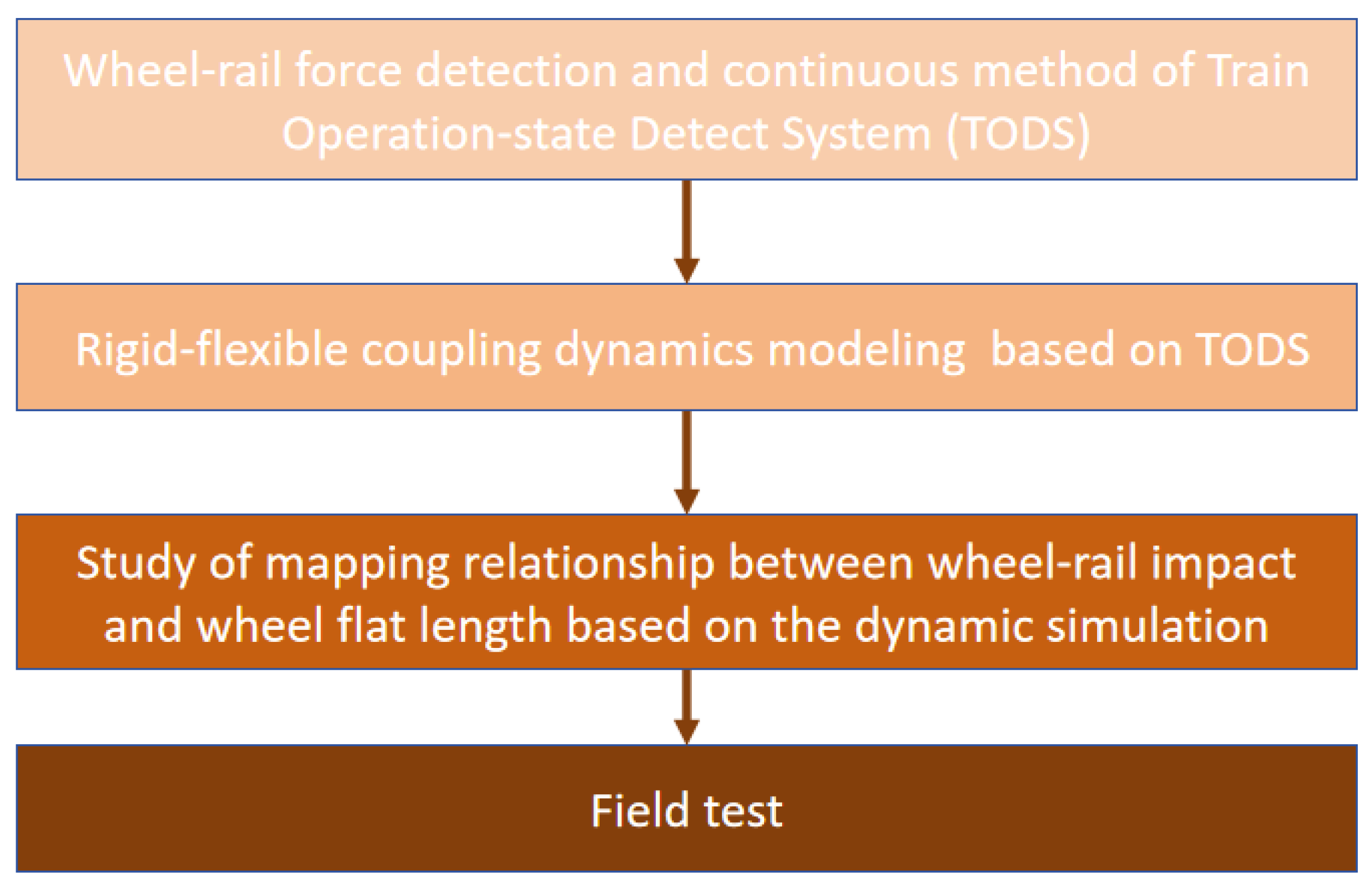
The paper’s structure is outlined in Figure 2:

Section 2 presents an overview of the Train Operation State Detection System (TODS), focusing on its wheel–rail force detection principle and discrete–continuous data reconstruction methodology.

Section 3 details the development of a rigid–flexible coupling dynamics model incorporating wayside wheel–rail force detection devices.

Section 4 investigates the characteristic mapping between wheel–rail impact responses and wheel flat parameters using simulation results.

Section 5 validates the theoretical relationships derived in Section 4 through field tests, analyzing real-world wheel–rail force data collected by on-site detection equipment.

2. Wheel–Rail Force Detection and Concatenation Method of Train Operation State Detect System (TODS)

Wheel–rail force detection methods are categorized into vehicle-mounted and wayside systems. Due to spatial limitations, wheel–rail forces measured on the track generally exhibit discrete and intermittent characteristics. In contrast, wheel–rail forces measured via vehicle-mounted sensors are typically continuous in both spatial and temporal dimensions. For wheel fault identification, wayside detection offers the most cost-effective solution. By attaching strain gauges to the rail web, this method measures wheel–rail forces within the span between two sleepers [31]. An alternative approach involves replacing sleepers with force sensors to monitor vertical forces at specific rail intervals. Among these, the shear strain gauge method is particularly efficient and economical, prompting extensive targeted research by scholars in recent years [32,33,34,35,36]. However, a critical limitation exists: the shear method can only capture wheel–rail forces within a single sleeper span. As a train passes through the detection zone, the collected data reflects only a small segment of the wheel tread. To overcome this, multiple detection zones are required so that combined data from all channels can cover the entire wheel circumference. Data from these parallel channels must then be integrated into a unified system, concatenated according to temporal and spatial sequences, to reconstruct continuous wheel–rail force profiles for each wheel.

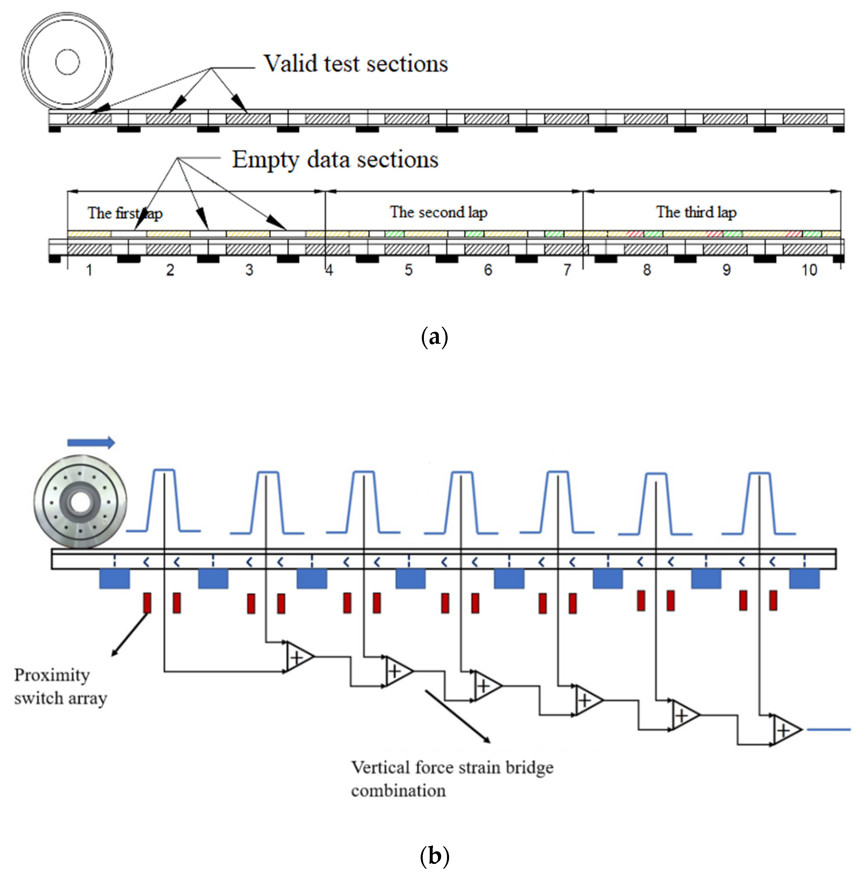
Figure 3 illustrates TODS’ wheel–rail force concatenation principle. The system employs the shear force method across 14 consecutive rail spans. For railway freight car wheels with a diameter of 840 mm, it has been proven that 14 test sections can cover the entire wheel surface [31]. As a wheel traverses the effective detection zone, each segment measures a partial wheel surface profile, followed by a data-free “blank zone” where no force monitoring occurs. During the first wheel rotation, the combined test zones cannot fully cover the entire tread. To achieve complete surface detection, the system extends the cumulative detection length, through proximity switch to detect the exact time when wheel entry/exit the detection zone, and split the data of each channel between the time, and then join the data in a single vector, and finally generate a complete, continuous wheel–rail force profile for each wheel.

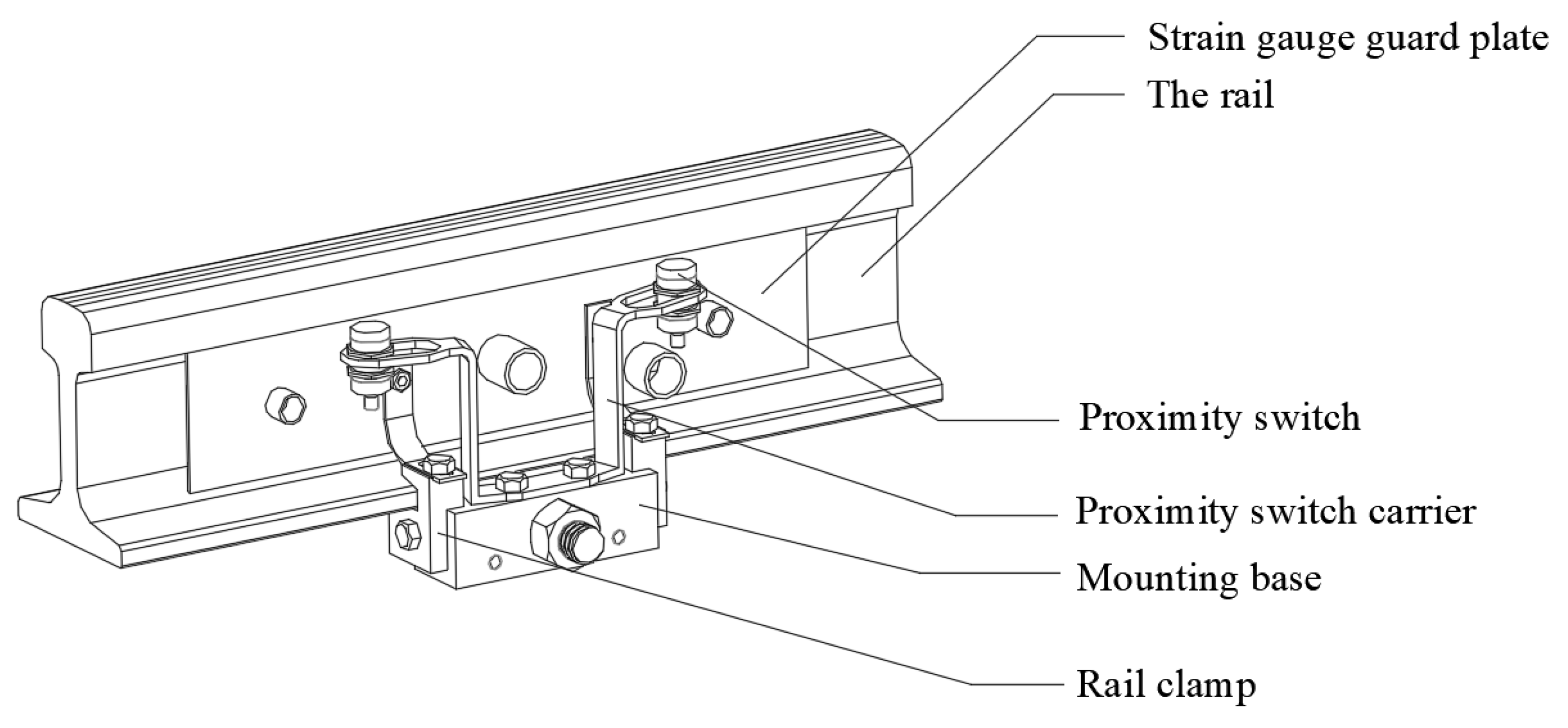
Figure 4 illustrates the rail-mounted proximity switch configuration. The sensing assembly is integrated into a custom-designed fixture comprising three rail clamps, a mounting base, a proximity switch carrier, two proximity switches, and two strain gauge guard plates. The entire fixture is anchored via the mounting base. The proximity switches are mounted on the carrier with a longitudinal center-to-center spacing of 240 mm, positioned directly above the shear measurement points on both rail sides. The switch tops are maintained at a 45 mm vertical clearance from the rail surface to ensure safety against rolling stock gauge intrusions. The proximity switch carrier attaches to the mounting base through two bottom circular holes, while the fixture secures to the rail foot via two bottom rail clamps and one opposing side clamp. As a wheel traverses the detection zone, the proximity switches record entry and exit timestamps. These timestamps enable the extraction of zone-specific wheel–rail force data, which are then temporally aligned and concatenated with data from adjacent segments (see Figure 4), forming a complete circumferential force profile. This design offers dual advantages: it avoids structural modification of the track and rail (since it is a non-intrusive installation method), ensuring low installation cost, while enabling simultaneous detection of additional wheel defects such as misalignment.

3. Rigid–Flexible Coupling Dynamics Model Based on TODS

To analyze the relationship between wheel faults and dynamic responses using TODS’ discrete wheel–rail force concatenation method, a vehicle–elastic track coupling dynamics model was developed using multi-body dynamics software (SIMPACK 2018) and finite element software (ANSYS 17.0). Figure 5 shows the vehicle–track coupling dynamics modeling diagram. In this model, wheels and rails are treated as flexible bodies: finite element mesh models were first created in ANSYS and then imported into SIMPACK for co-simulation. The carbody is modeled as a rigid body, excluding onboard equipment vibrations. The rail support system employs discrete supports, incorporating under-sleeper stiffness and rail fastener properties, while the truck’s elastic suspension nonlinearities are fully considered.

The vehicle model comprises 90 degrees of freedom (DOF):

Carbody, four side frames, two bolsters: Each with six DOF (three translational, three rotational).

Eight bearing saddles: Each with one vertical DOF.

Four wheelsets: Each with six DOF (three translational, three rotational), one bending DOF, and 1 torsional elastic DOF.

Eight wedges: Each with one vertical DOF.

Nonlinear wheel–rail contact geometry is integrated into the model. Key vehicle parameters are listed in

Table 1. Main values of parameters involved in the dynamic model.

Parameters	Units	Values
Carbody mass	kg	10,297
Bogie mass	kg	5485
Wheelset mass	kg	1171
Wheelset diameter	m	0.84
Bogie distance	m	8.2
Wheel base	m	1.83
Squeeze spring stiffness	MN/m	0.275
Axial stiffness of intertie	MN/m	14.8
Stiffness of primary suspension along the x-axis	MN/m	13
Stiffness of primary suspension along the y-axis	MN/m	11
Stiffness of primary suspension along the z-axis	MN/m	160
Stiffness of secondary suspension along the x-axis	MN/m	3.127
Stiffness of secondary suspension along the y-axis	MN/m	3.127
Stiffness of secondary suspension along the z-axis	MN/m	4.235
Carbody inertia about the x-axis	kg·m2	1.45 × 104
Carbody inertia about the y-axis	kg·m2	1.06 × 105
Carbody inertia about the z-axis	kg·m2	1.07 × 105
Length of flexible rail	m	12
Type of rail	kg/m	60
Stiffness of sleeper suspension along the x-axis	MN/m	40
Stiffness of sleeper suspension along the y-axis	MN/m	60
Stiffness of sleeper suspension along the y-axis	MN/m	160
Damping of sleeper suspension along the x-axis	Ns/m	1000
Damping of sleeper suspension along the y-axis	Ns/m	1000
Damping of sleeper suspension along the z-axis	Ns/m	10,000

. Wheel flat lengths are varied between 10 and 70 mm, and vehicle speeds between 10 and 80 km/h. The track model uses an elastic discrete support framework, where rail-under support elements represent fasteners and ballast layers.

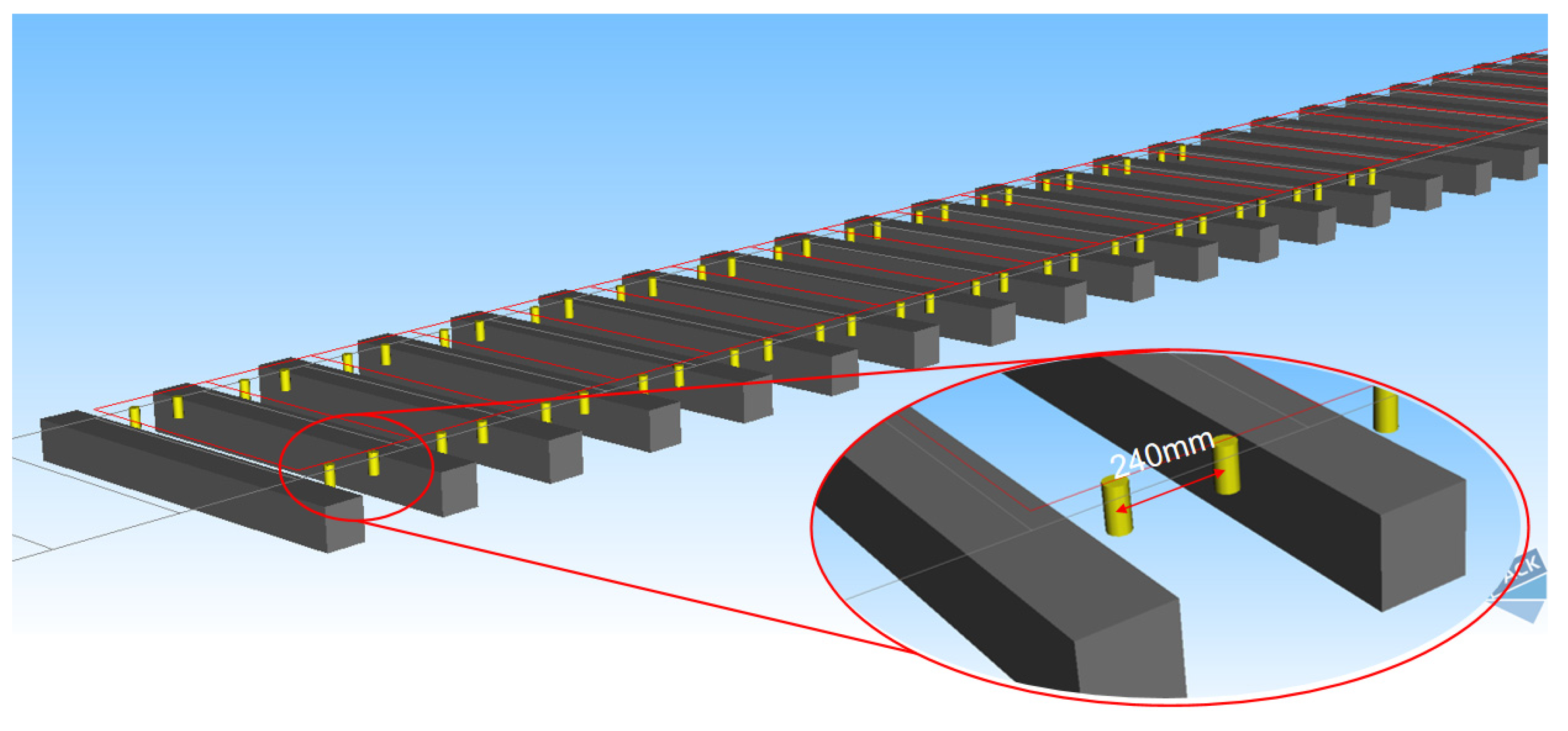
The hybrid coordinate system method was employed to model wheel elastic deformations while excluding the effects of parametric resonance from vehicle equipment. To generate wheel–rail force outputs consistent with field data collected by the TODS, a series of pressure sensors (a measurement module in SIMPACK, which can be understood as a data-readout tool) were integrated into the track model at 240 mm intervals between sleepers, as depicted in Figure 6. This sensor configuration enables precise timing of wheel passage through each detection zone, facilitating subsequent concatenation of discrete wheel–rail force measurements.

Wheel flats can be categorized into new flats and old flats. The geometry of a new wheel flat approximates a circular chord, though idealized new flats are rarely observable in practice. Once a flat forms, continued train operation rapidly rounds the flat’s sharp edges, transforming it into an old flat. For this reason, simulation analysis focuses on establishing a mathematical model of old flats to reflect real-world wear characteristics.

The formula for flat irregularity Z_p is as follows [37]:

$$Z_p={\displaystyle \frac{1}{2}}h\left[1-\cos \left({\displaystyle \frac{2\pi x}{L}}\right)\right]$$

(1)

where h = 2L/(16R);

L is the length of the wheel flat;

R is the radius of the wheel rolling circle;

x is the arc length along the wheel surface.

The wheel flat can be converted into the change in wheel radius, as follows:

$$R\left(\beta \right)=R-{\displaystyle \frac{R{\alpha }^2}{8}}\left[1-\mathrm{c}\mathrm{o}\mathrm{s}\left({\displaystyle \frac{\pi }{\alpha }}\beta \right)\right]$$

(2)

where α = L/(2R);

β is the wheel rotation angle.

The established old flat model describes wheel radius variations as a function of both flat length and wheel rotation angle. The relationship between wheel flat depth and length is illustrated in Figure 7.

With the vehicle–elastic track coupling dynamics model finalized, numerical simulations are conducted to derive the mapping relationship between wheel defects and wheel–rail forces, enabling reverse fault identification research.

4. Wheel Flat Shock Effect and Its Mapping Relationship

Figure 8 presents wheel–rail force simulation results for a 30 mm flat at 50 km/h. The vehicle traverses the elastic track segment between 0.7 and 1.7 s, revealing distinct wheel–rail force characteristics between elastic and non-elastic rail sections. The wheel flat induces periodic impact forces: when the flat length is 30 mm and speed reaches 80 km/h, the peak wheel–rail force reaches 150 kN—approximately six times the static wheel–rail force (≈25 kN). Under higher vehicle loads or speeds, these impacts could theoretically exceed current magnitudes.

Continuous periodic impact is a defining characteristic of wheel flat faults. Figure 8 illustrates continuous wheel–rail force profiles under a flat condition, but the TODS measures discrete wheel–rail forces. The model’s displacement sensor outputs mimic vehicle passage signals (as an alternative to the proximity switch in the simulation model), as shown in Figure 9. To align with real-world wayside detection data, discrete wheel–rail forces from the simulation model are processed, as depicted in Figure 10.

The top of Figure 10 shows the continuous wheel–rail force signal measured by the on-board wheel–rail force testing unit in SIMPACK. By combining the time when the vehicle enters/leaves the valid sections (such as the signal shown in Figure 9), the continuous wheel–rail force signal can be segmented according to the time of the effective testing interval, resulting in the discrete wheel–rail force signal shown in the middle of Figure 10. Finally, the discontinuous, discrete wheel–rail force signals in Figure 10 are connected in the same time domain, yielding the simulated concatenation wheel–rail force signal at the bottom of Figure 10, which is consistent with TODS.

The bottom plot demonstrates that while TODS cannot provide continuous impact profiles like onboard systems, its full-circumference coverage ensures at least one impact signal per wheel rotation. This allows for identifying wheel damage and estimating flat length via detected impact signatures.

By analyzing the wheel–rail impact–flat parameter mapping through this wayside force simulation model, the reliability of subsequent wheel fault identification in wayside detection systems is fundamentally ensured.

By extracting peak wheel–rail forces for all wheel flat conditions under empty vehicle operation, a force–speed relationship curve is generated (Figure 11). As previously discussed, wheel–rail impact forces decrease proportionally once the vehicle exceeds the critical speed, whereas forces increase with speed below this threshold. Notably, a near-linear relationship exists between impact force magnitude and wheel flat length. The force–speed curve in Figure 11 is fitted using polynomial regression to quantify this relationship.

In practical scenarios, wheel flat impacts on the track are most pronounced and damaging under loaded conditions. Therefore, analyzing flat-induced forces in heavy-load scenarios is critical.

Under heavy load, the vehicle dynamics model undergoes parameter adjustments compared to the empty state, primarily in carbody mass, center of gravity (CG) position, and bolster CG position (

Table 2. Changed values of parameters involved in the heavy load dynamic model.

Parameters	Units	Values
Carbody mass	kg	90,297
Center of gravity position of carbody (from rail surface)	m	2.232
Carbody inertia about x-axis	kg·m2	2.163 × 105
Carbody inertia about y-axis	kg·m2	9.963 × 105
Carbody inertia about z-axis	kg·m2	9.839 × 105
Center of gravity position of the pillow (from the rail surface)	m	0.506
Lateral stiffness of the second suspension (end of bolster)	MN/m	3.127
Vertical stiffness of the second suspension (end of bolster)	MN/m	3.127
Longitudinal stiffness of the second suspension (end of bolster)	MN/m	4.235

). The elastic wheelset and track models are retained, with other dynamics parameters remaining consistent with the empty vehicle model.

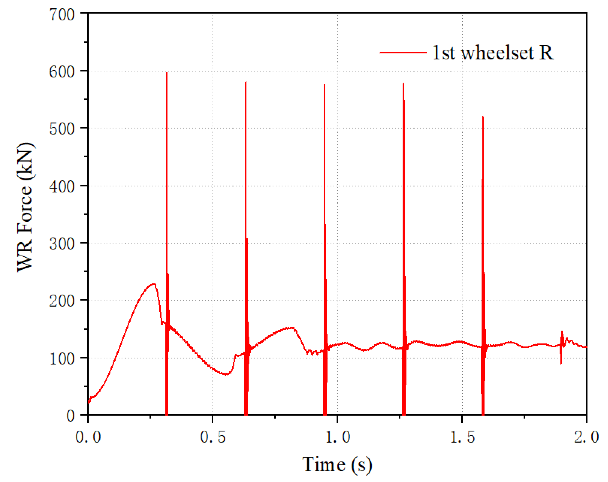
Figure 12 presents wheel–rail force simulation results for a 50 mm wheel flat under heavy-load conditions at 30 km/h. Correspondingly, the vehicle traverses the elastic track region between 0.6 and 1.7 s. Under heavy load, a 50 mm flat at 30 km/h generates a peak wheel–rail impact force of 596 kN—4.768 times the static wheel–rail force and 3.97 times the impact force under empty-load conditions. By extracting all peak forces, the force–speed relationship plot in Figure 13 is generated.

Under heavy-load conditions, wheel–rail force peaks exhibit a similar trend to the empty-load model: an initial increase with speed, followed by a decrease. Notably, force growth with speed is less steep in loaded conditions, reaching a maximum at approximately 50 km/h before declining. As with the empty-load case, a near-linear relationship persists between impact force magnitude and wheel flat length.

To improve the applicability of practical engineering applications, it is necessary to obtain the mapping relationship between fault responses and fault characteristics. This mapping relationship can be derived by fitting the curves of wheel–rail impact force changes under different fault conditions. In real-world detection, vehicle speed can be accurately captured by speed sensors. Balancing computational constraints and curve-fitting precision typical in engineering applications, a two-step fitting approach was adopted: first, wheel–rail force was curve-fitted against wheel flat length; then, the coefficients of the initial fitting function were further regressed with vehicle speed. This iterative process yielded a comprehensive fitting function relating wheel–rail force to both flat length and vehicle speed.

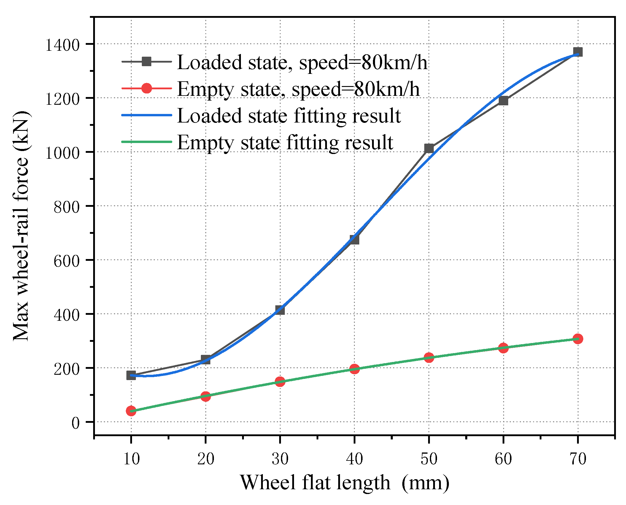
Simulations were conducted on empty and loaded vehicles, each featuring a flat on the right front wheel of the leading bogie, with a fixed speed of v = 80 km/h. Considering the trade-off between simulation accuracy and available computational resources, a second-order polynomial was employed for curve fitting of empty vehicle data, while a third-order polynomial was applied to loaded vehicle data. The fitting result is shown in Figure 14, where both empty load state and loaded state show a good mapping result.

Figure 15 displays the fitted contour curves for empty and heavy vehicles. Across the speed range v = 10~80 km/h, the vertical wheel–rail force of empty vehicles monotonically increases with wheel flat length. Under heavy-load conditions, at low speeds, the vertical force first decreases and then increases with flat length, whereas at high speeds, it increases monotonically with flat length. Within the flat length range from 10 mm to 70 mm, the vertical force for both vehicle types exhibits a non-monotonic speed dependence, first increasing, then decreasing, and subsequently increasing again as speed changes. Notably, heavy vehicles show more pronounced vertical force variations compared to empty vehicles.

The figure demonstrates excellent curve-fitting performance, with randomly selected wheel–rail impact forces for both vehicle types falling within a 5% error margin of the fitted curves. This two-step fitting method was applied to impact forces across all tested speeds. The fitting curve formula for the empty vehicle is shown in Equation (3), and the fitting curve formula for the loaded vehicle is shown in Equation (4), yielding the corresponding coefficients in

Table 3. Fitting curve coefficient (for empty state(0 t load)/loaded state(80 t load)).

Speed	Empty State				Loaded State
	a1	b1	c1	R2	a2	b2	c2	d2	R2
10 km/h	347.31	−4.59	51,859.01	0.11179	−9.06	0.46	−0.01	151,928.64	0.86765
20 km/h	7142.32	−4.47	−25,553.03	0.99985	4608.56	40.76	−0.01	116,433.04	0.99775
30 km/h	6182.02	36.77	−27,859.61	0.99948	4119.41	283.03	−2.26	103,812.61	0.99952
40 km/h	3295.36	72.93	−2877.44	0.99922	8906.73	295.85	−2.35	51482.71	0.99744
50 km/h	1414.32	79.24	19,869.62	0.99914	3402.04	536.77	−4.13	85,707.04	0.99717
60 km/h	515.38	71.54	39,936.31	0.99381	−1441.68	516.16	−3.12	123,085.14	0.99794
70 km/h	3155.03	23.98	16,795.12	0.98799	−12,913.77	809.08	−5.66	215,367.14	0.99839
80 km/h	6407.69	−24.34	−22,307.21	0.99982	−26,291.14	1290.74	−10.03	316,469.57	0.99805

.

$$F=a_1{L}^2+b_{1}L+c_1$$

(3)

$$F=a_2{L}^3+b_2{L}^2+c_{2}L+d_2$$

(4)

Here, F denotes the wheel–rail force, L denotes the length of wheel flat, a₁, b₁, c₁ denote the fitting coefficients for empty vehicles, while a₂, b₂, c_2, and d₂ apply to loaded vehicles.

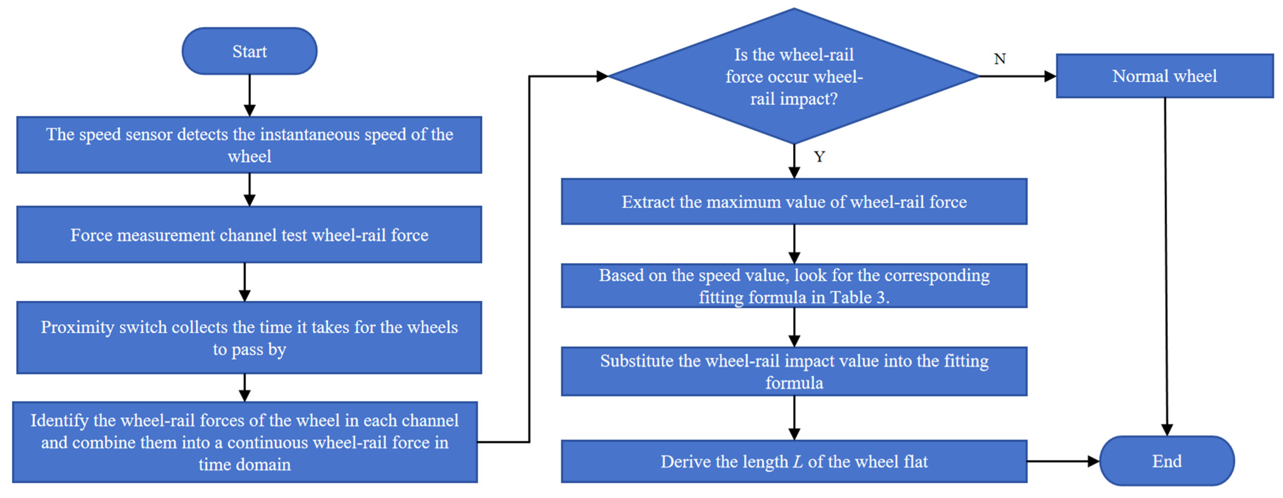
According to the mapping relationship, by combining the vehicle speed measured by the TODS equipment and the wheel–rail force impact value, the flat length of the wheel can be deduced. The data processing process is shown in Figure 16. When the speed is not an ideal value (such as 56 km/h), the interpolation method can be used; that is, after calculating the values of adjacent speeds (such as 50 km/h and 60 km/h), perform the interpolation method to obtain the flat length under the corresponding speed condition.

5. Field Test and Discussion

To validate the reliability of the identification algorithm, the developed Train Operation State Detection System (TODS) was deployed on an operational railway line. The test site is located approximately 2 km from the Suning North Station of the Shuohuang Heavy-Haul Railway, where the average passing vehicle speed is around 40 km/h. The TODS wheel–rail impact detection system was installed on the upstream track, focusing on fully loaded trains.

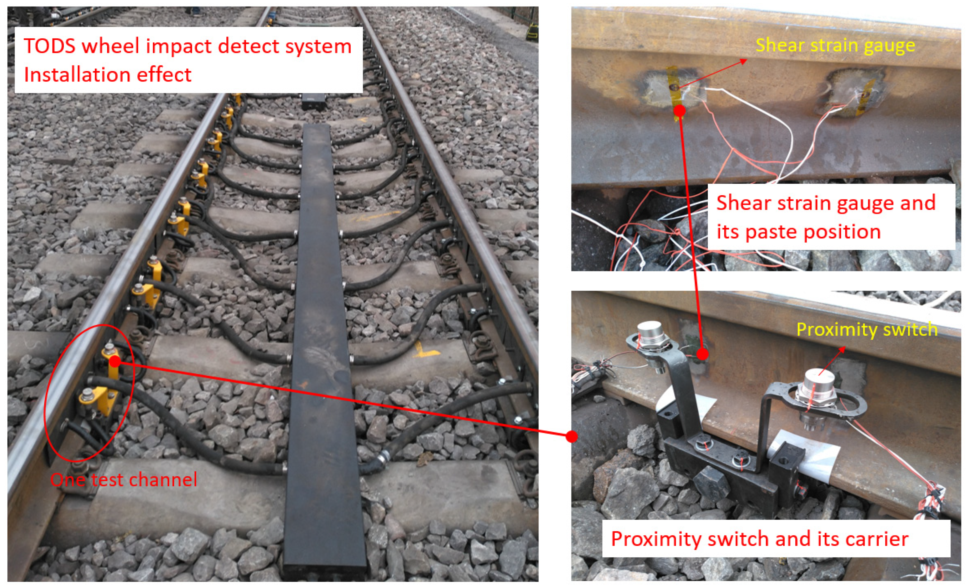
Shear strain gauges were strategically mounted on both the left and right rails to measure wheel–rail forces. The installation encompasses 14 rail spans. Each measuring point consists of four strain gauges, which are combined through a bridge circuit to form one measuring point. One rail span has two measuring points (one on the left and one on the right), utilizing a total of 28 strain gauge channels. Additionally, a proximity switch was affixed to one side of the rail, serving as a trigger to accurately record the precise moments when wheels enter and exit the detection zone.

Table 4. The relevant parameters of the strain gauge and proximity switch.

Strain Gauge		Proximity Switch
Size	10 mm × 4.6 mm	Thread type	M30 × 1.5
Coefficient of thermal expansion	10.8 × 10−6/K	Switching frequency	≤90 Hz
Operating temperature range	−30~40 °C	Delay response	≤6 × 10−5 ms
Maximum permissible effective bridge voltage	13 V	[Us] rated supply voltage	12~24 V DC
Nominal resistance	120 Ω	[Sn] nominal sensing distance	40 mm
GF	1.8

details the key parameters of the strain gauges and proximity switch, while Figure 17 illustrates the actual installation configuration.

Figure 18a depicts the wheel–rail force signal captured by a single vertical force measurement channel of the TODS. Notably, each peak in the figure represents the wheel–rail force exerted when a wheel traverses the load-measuring bridge; these peaks correspond to individual wheels rather than continuous, discrete forces from a single wheel across different spatial positions. As a result, the time intervals between successive wheel–rail force signals are irregular. Leveraging the known inter-wheel distance of 1.83 m within a bogie, the vehicle’s running speed was calculated to be 59.89 km/h. The algorithm processes the spatially ordered discrete wheel–rail forces generated by the same wheel, utilizing the wheel passage sequence and proximity switch signals, as illustrated in Figure 18b.

From Figure 18b, it is evident that when a wheel passes through the detection area, the responses of each force-measuring channel occur in a precise spatiotemporal sequence with consistent time intervals. The top data from all test channels exhibit smooth characteristics, free of any impact-induced anomalies or signal burrs.

The wheel–rail force profile obtained through the concatenation method is presented in Figure 19. The data reveals that the fluctuations in the wheel–rail force remain within the normal operational range, devoid of significant burrs or wheel–rail impact signatures. This observation strongly suggests that the wheel is in excellent condition, free from surface defects such as wheel flats; it serves as excellent comparative data for the faulty wheel data. With a wheel–rail force magnitude of approximately 120 kN, it can be deduced that the vehicle is operating under a full-load condition, corresponding to a payload of around 76 t.

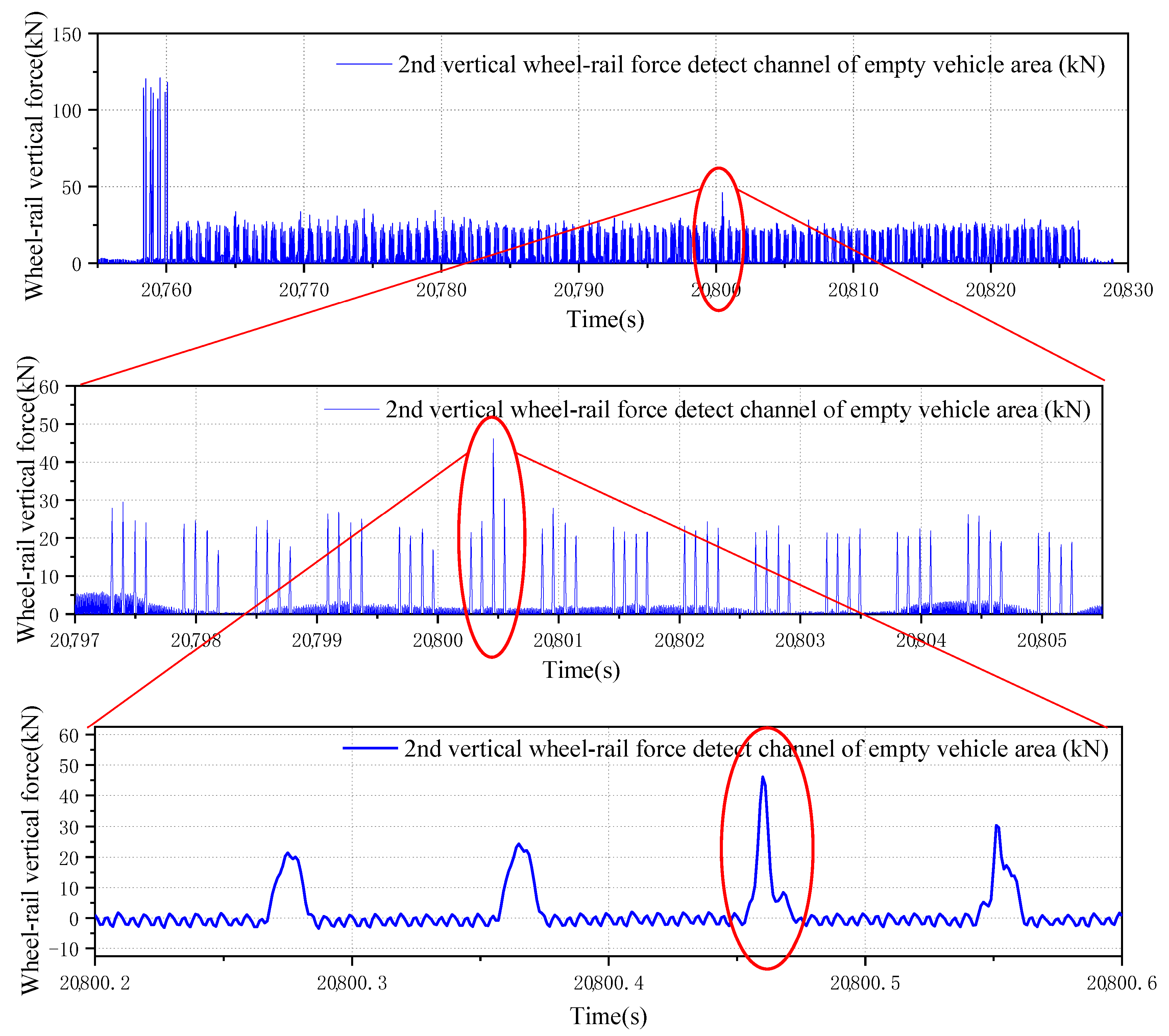
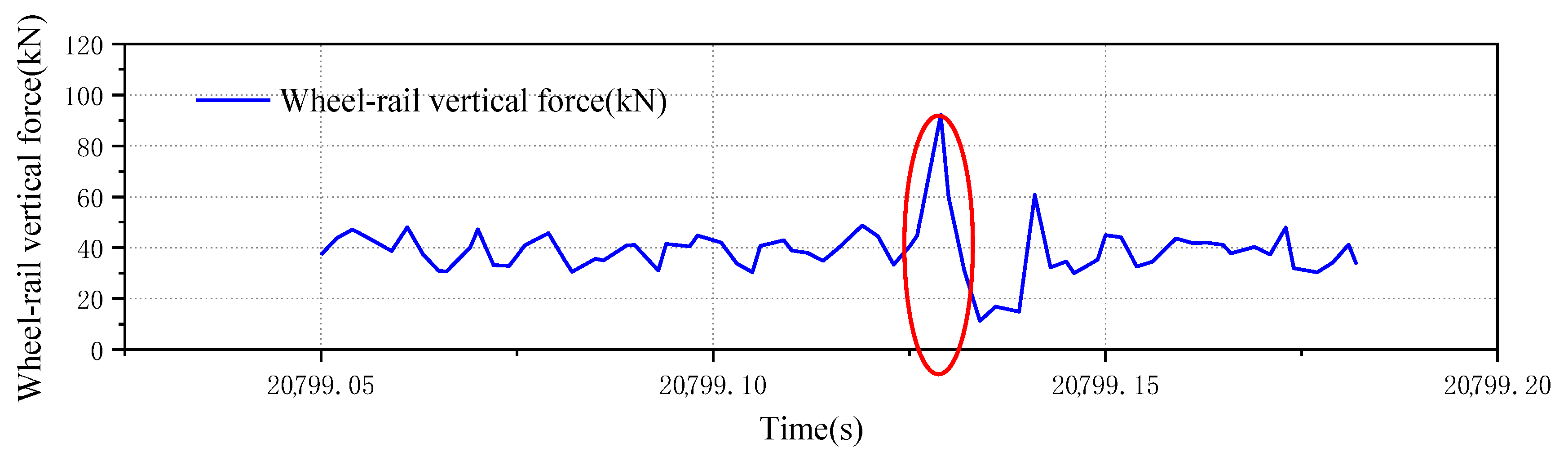
Figure 20 illustrates an abnormal wheel–rail force signal detected by the No. 2 left-side wheel–rail vertical force channel in an empty car line, with the channel positioned on the right side relative to the incoming vehicle direction. A magnified view of the wheel–rail impact reveals that the abnormal force signature originates from wheel tread damage. Retrieve all the wheel data of this wheel from all channels and connect them in the time domain; the continuous wheel–rail force results can be obtained, as shown in Figure 21.

The vehicle speed during this test was 59.89 km/h, with a maximum wheel–rail impact force of 46.1 kN. The average wheel–rail force of 25 kN confirms an empty-load condition. Leveraging the wheel flat mapping relationships and linear interpolation method established in Section 4 for heavy-haul trains, the calculated flat length for this wheel is approximately 4.2 mm.

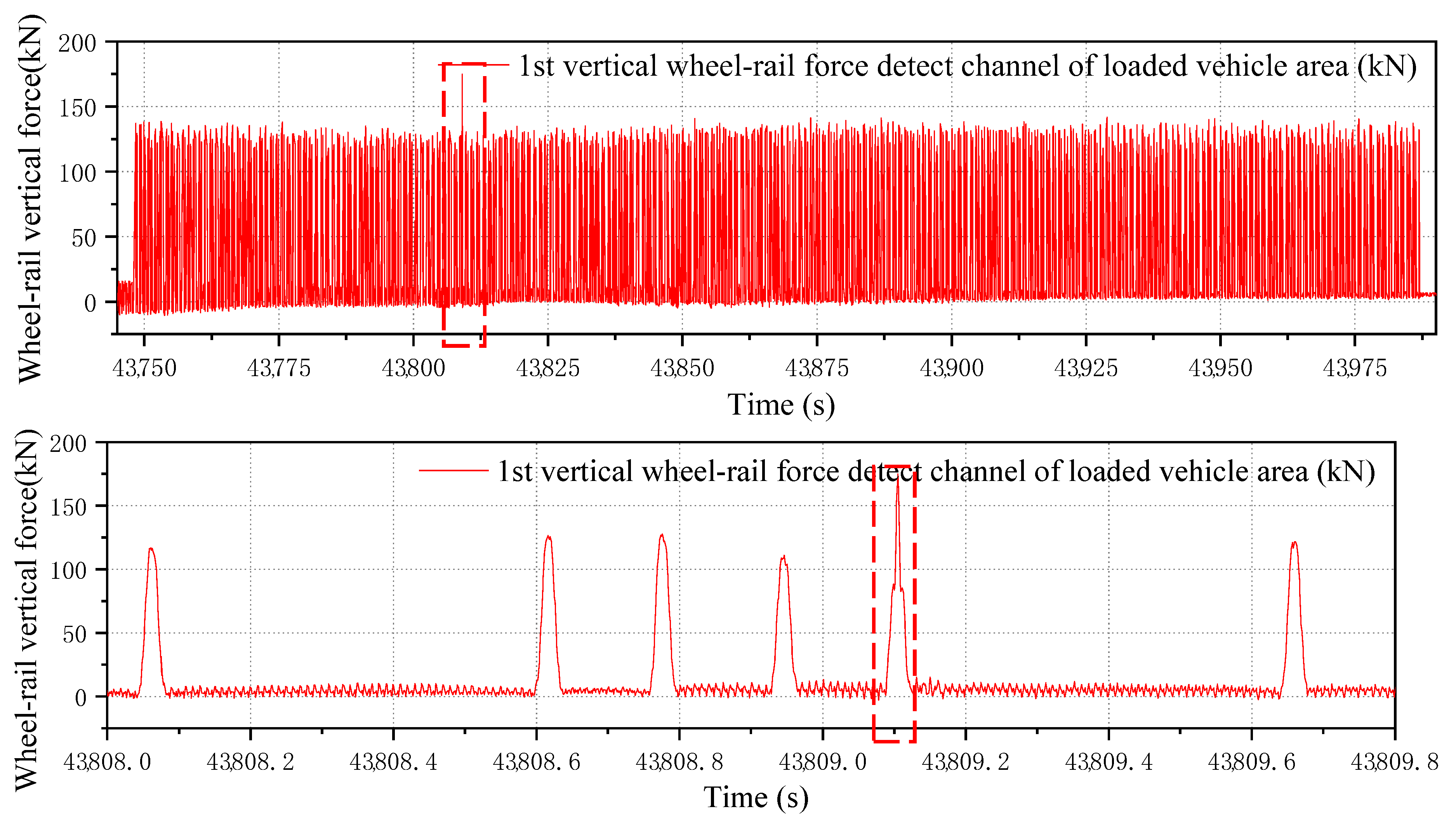
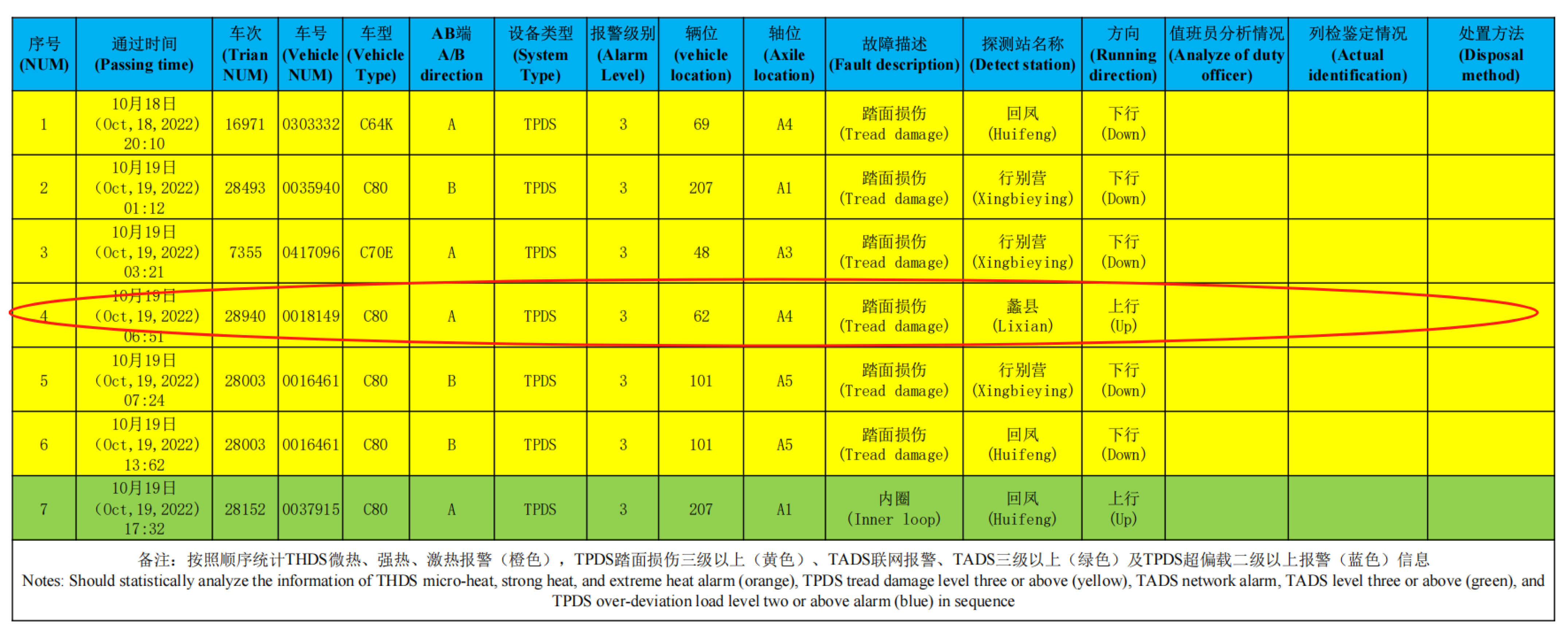
Figure 22 displays the wheel–rail force signal of an abnormal train experiencing a wheel–rail impact. The vehicle was operating under fully loaded conditions, with the wheel generating an impact equivalent of 1.397 and a maximum impact force of approximately 170 kN—prompting the system to trigger a warning signal. Tracking records indicate the train number was 28,940, the vehicle number 0018149, and the vehicle type C80, with a passing time of 07:26 on 19 October 2022. System measurements recorded a running speed of 41.2 km/h and an average axle load of 24.3 t for this vehicle.

Substituting the impact parameters into the mapping relationship established in Section 4, the calculated wheel flat length is 7.3 mm. Cross-referencing with the TPDS (Truck Performance Detection System) alarm data on the same route (Figure 23) reveals consistent alarm timing and impact characteristics. The vehicle number, train number, and vehicle type all match perfectly between the two systems, validating the reliability of TODS’ detection results.

The wayside detection system has been in field tests for 10 days (from 17 October to 27 October 2022), continuously monitoring passing vehicles with extensive data acquisition. In total, it has detected 465 trains comprising 56,265 vehicles, 225,060 wheelsets, and 450,120 wheels, with the C80 vehicle type constituting the majority. During this period, the system captured 20 wheel–rail impact events, including 4 from downstream trains and 16 from upstream trains. The fault alarm statistics are summarized in

Table 5. Alarm forecast of wayside detection system (data from 17 October to 27 October 2022).

Number	Date	Time	Type	Vehicle Number	Fault Location	Alarm Classification
1	17 October	16:34	C80	0018149	Right of the 2nd wheelset	Warning
2	18 October	09:06	C80	0024047	Right of the 3rd wheelset	Warning
3	19 October	07:26	C80	0018149	Right of the 2nd wheelset	Warning
4	23 October	16:52	C80	0026293	Right of the 3rd wheelset	Warning
5	23 October	12:53	C80	0028830	Left of the 1st wheelset	Warning
6	24 October	15:34	C80	0039023	Right of the 2nd wheelset	Warning
7	24 October	13:33	C80	0014170	Left of the 1st wheelset	Warning
8	24 October	17:05	C64K	0415827	Left of the 3rd wheelset	Warning
9	24 October	17:24	C80	0024160	Left of the 3rd wheelset	Warning
10	24 October	14:33	C80	0016461	Left of the 3rd wheelset	Warning
11	24 October	17:05	C64K	0354058	Right of the 4th wheelset	Warning
12	26 October	18:02	C80	0027758	Left of the 1st wheelset	Warning
13	26 October	12:20	C80	0017694	Left of the 4th wheelset	Warning
14	26 October	13:34	C70A	0030607	Left of the 3rd wheelset	Warning
15	27 October	15:29	C80	0024851	Left of the 4th wheelset	Warning
16	27 October	11:50	C80	0024146	Left of the 2nd wheelset	Warning

.

6. Discussion

Due to safety considerations from railway operation units, it is not possible to artificially arrange known wheel faults on normally operating trains. Currently, the TODS can only passively monitor the fault conditions of vehicles passing through the monitoring section, and fault tracing is rather difficult. The correctness can only be indirectly verified by comparing fault data with the TPDS system. In the subsequent research, ongoing optimization of fault algorithms and models using field data will enhance the accuracy of mapping relationships and improve the precision of detection results. More comprehensive and specific tests on the system from other aspects will constantly be conducted to verify the accuracy of the system detection algorithm.

7. Conclusions

Based on the impact mechanism of wheel flats and the detection principle of the wayside wheel–rail force detection system (TODS), this study investigates the fault conditions of wheel flats in heavy-haul railway freight cars, establishes a rigid–flexible coupling dynamics model of freight cars and flexible tracks, and simulates and validates the reliability of TODS’ wheel–rail force concatenation method. Through simulation, the mapping relationships between wheel flats and wheel–rail impacts under both full-load and empty-load conditions are obtained. Finally, field data was measured. Combining theoretical derivation, simulation, and field measurements, the following conclusions are drawn:

(1)

The wayside wheel–rail force acquisition system (TODS) is theoretically and simulation-verified. A detection section spanning 14 rail spans (covering an 840 mm wheel surface) ensures full circumferential coverage of wheel profiles.

(2)

Wheel flats induce periodic wheel–rail impacts. At low speeds (≤80 km/h), the magnitude of impact first increases with speed and then decreases. Heavier vehicle loads lower the critical speed at which maximum wheel–rail impact occurs.

(3)

A mapping relationship is established between wheel–rail impact parameters (e.g., peak force, impact equivalent) and wheel flat characteristics (length) across different speeds. By detecting impact equivalents, key flat parameters (e.g., length) can be inversely calculated through these relationships.

(4)

The TODS and the flat length deduction method have been applied to the operational railway line. Through a period of operation, good effects in monitoring wheel flats have been achieved. Indirect comparison with the detection results of the TPDS system has indirectly verified the effectiveness of the system. These findings provide theoretical and data-driven support for wheel flat identification and real-time fault monitoring.