
Computational Investigations and Control of Shock Interference †


Abstract
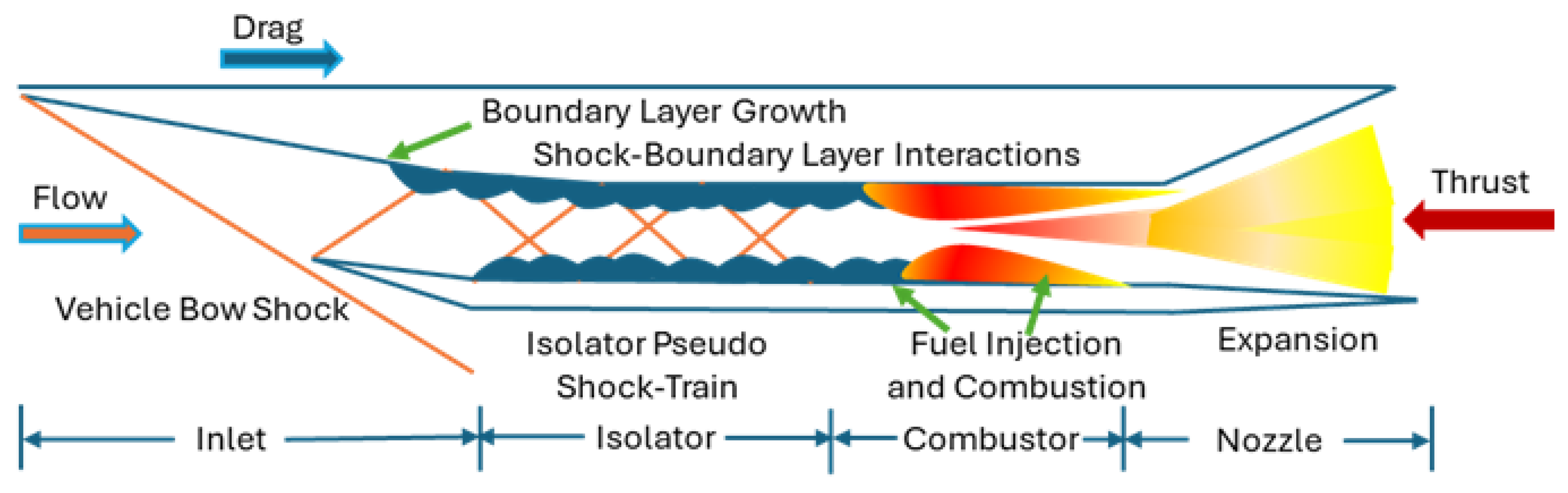
1. Introduction
1.1. Objectives
- To perform code verification and model validation with existing experimental data.
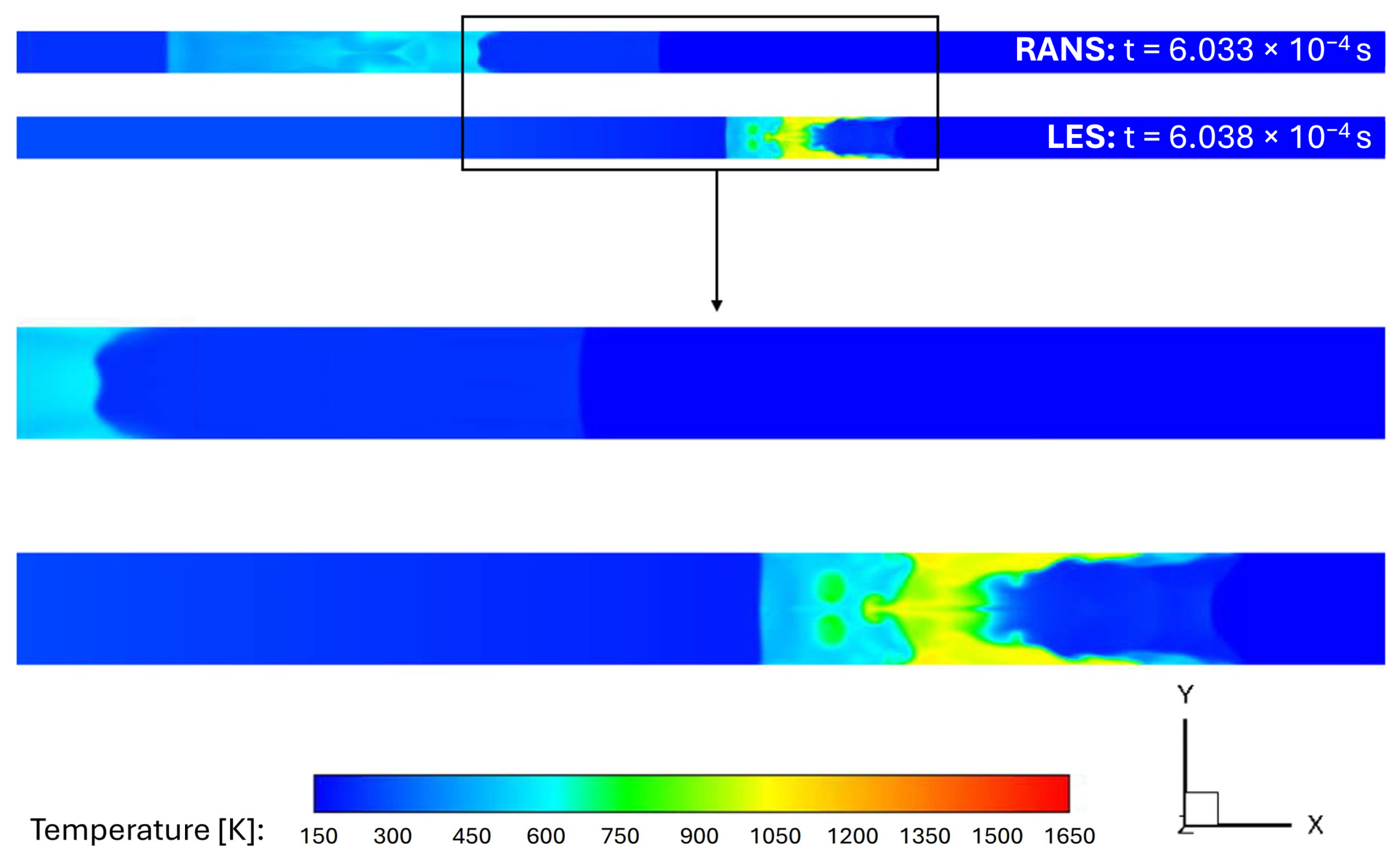
- To perform computational investigations of shock interference by utilizing both scale-resolving computational methods, such as large eddy simulation, and mean flow resolving methods, such as unsteady Reynolds Averaged Navier–Stokes method.
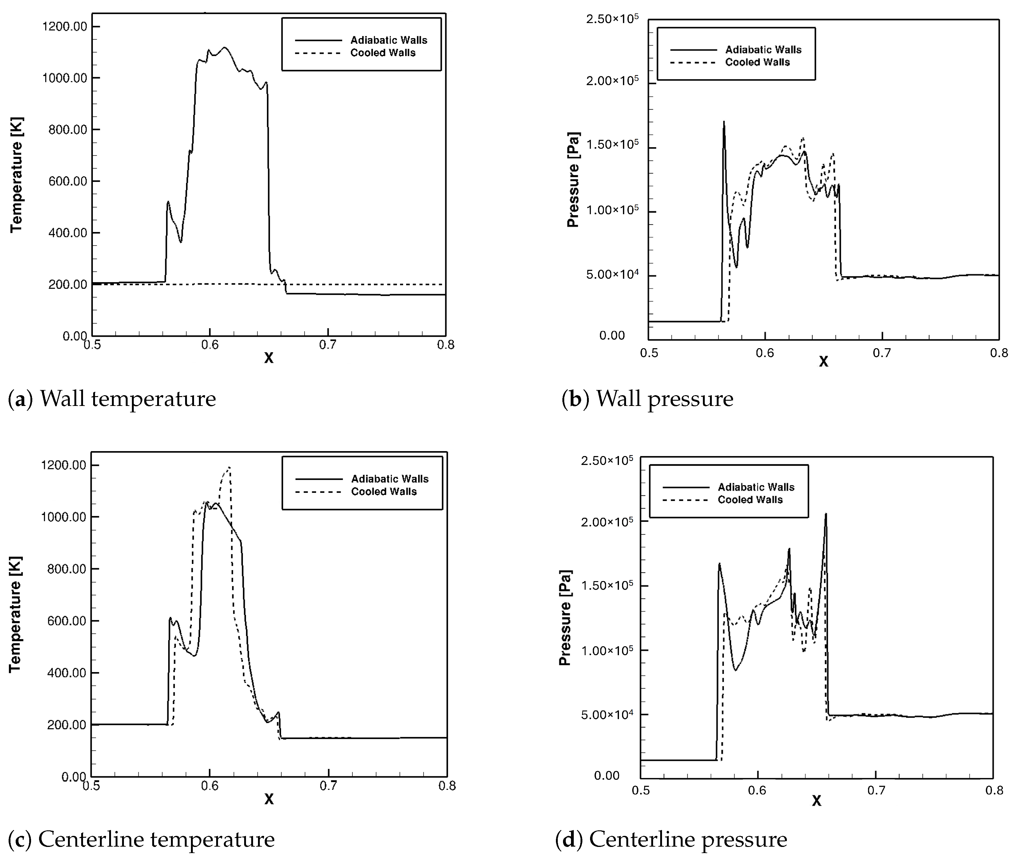
- To compare the effect of wall cooling on boundary-layer control for both backpressured isolator and modified shock-tube with crossflow.
1.2. Technical Approach
1.2.1. Computational Methods and Mesh
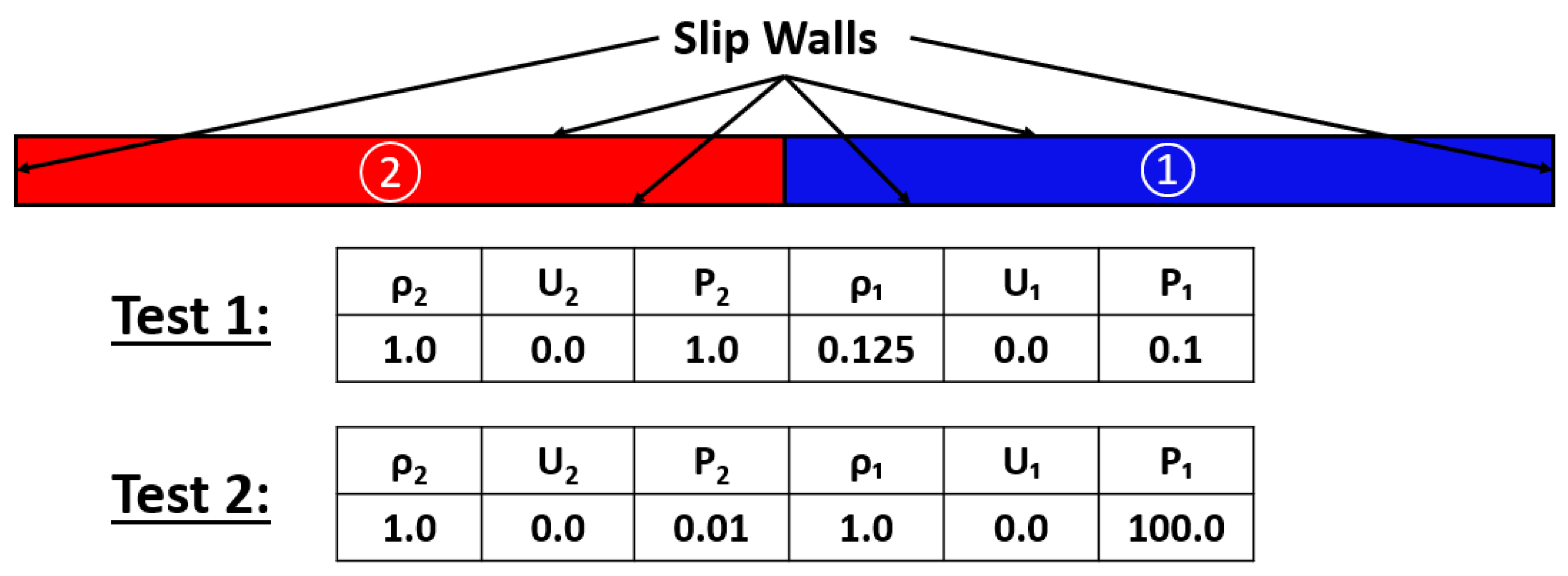
- Verification: A one-dimensional shock-tube problem, also known as Sod’s shock-tube problem [21] has been chosen for verification as the exact solution for this problem is known.
- Validation: A backpressured isolator from NASA Langley Research Center’s Isolator Dynamics Research Lab [22] has been utilized for model validation since the time-averaged measured wall pressures have been available.
- Demonstration and Investigation: Once the computational code and model have been verified and validated, a modified shock-tube (a shock-tube with square cross-section and open ends) has been utilized to investigate shock interference and interaction with boundary-layer phenomena. This shock-tube was modified to generate the effects of air entering an isolator from the inlet, and a pseudo-shock-train was generated due to the combustor backpressure and thermal choking.
1.2.2. Turbulence Closure Models
2. Code Verification
2.1. Mesh
2.2. Numerical Methods
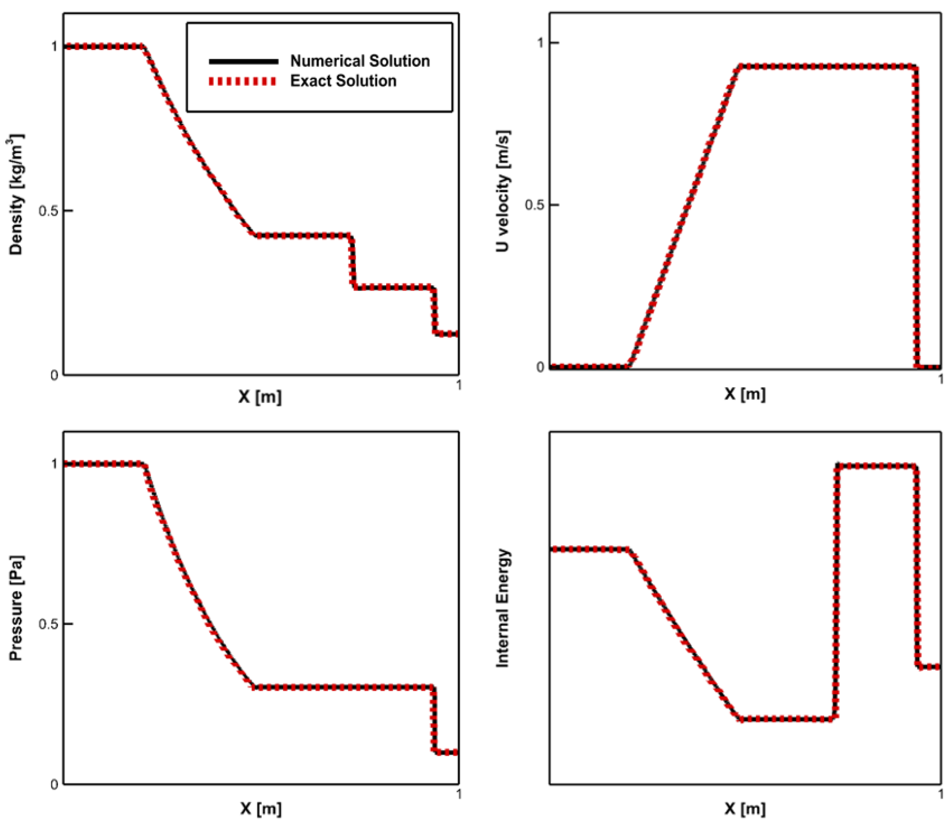
2.3. Results of Code Verification
3. Model Validation
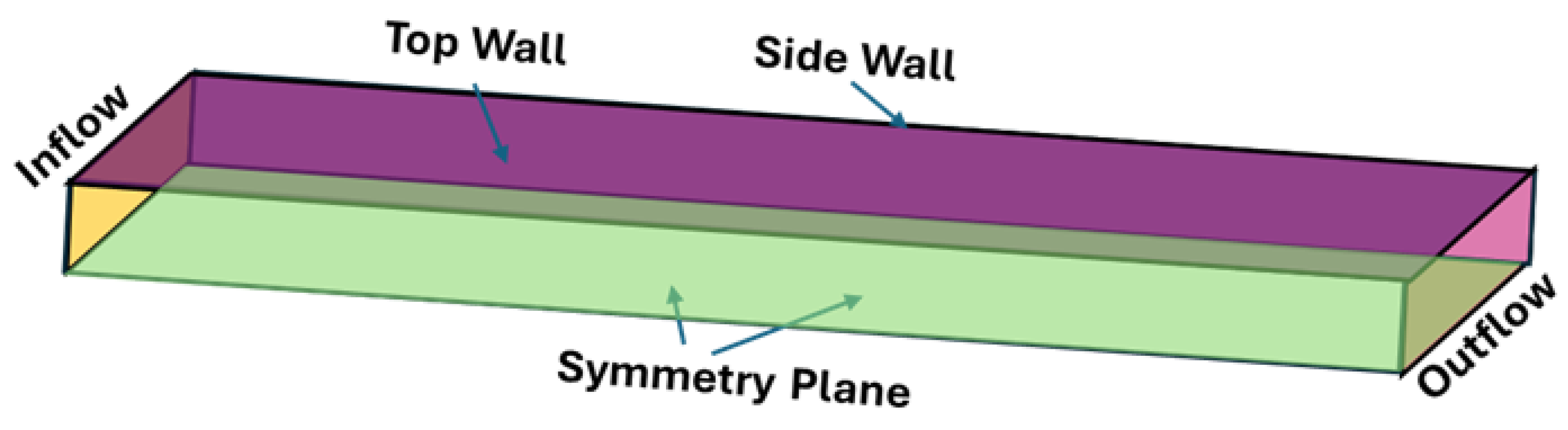
3.1. Computational Domain and Mesh
3.2. Numerical Methods
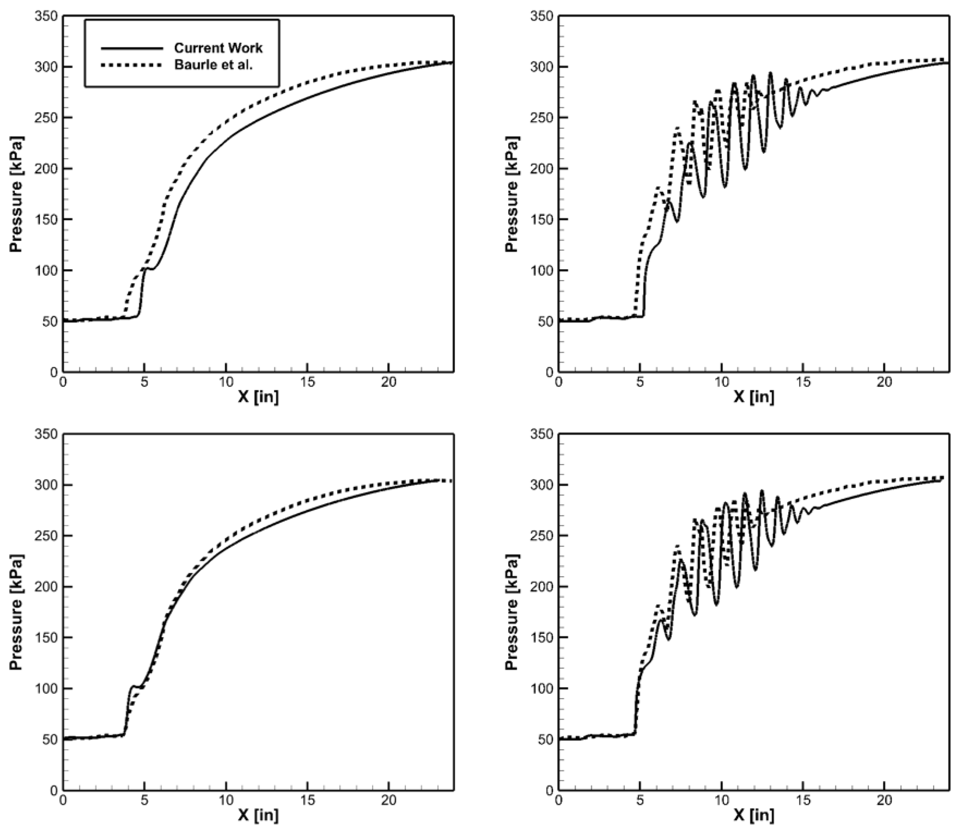
3.3. Results
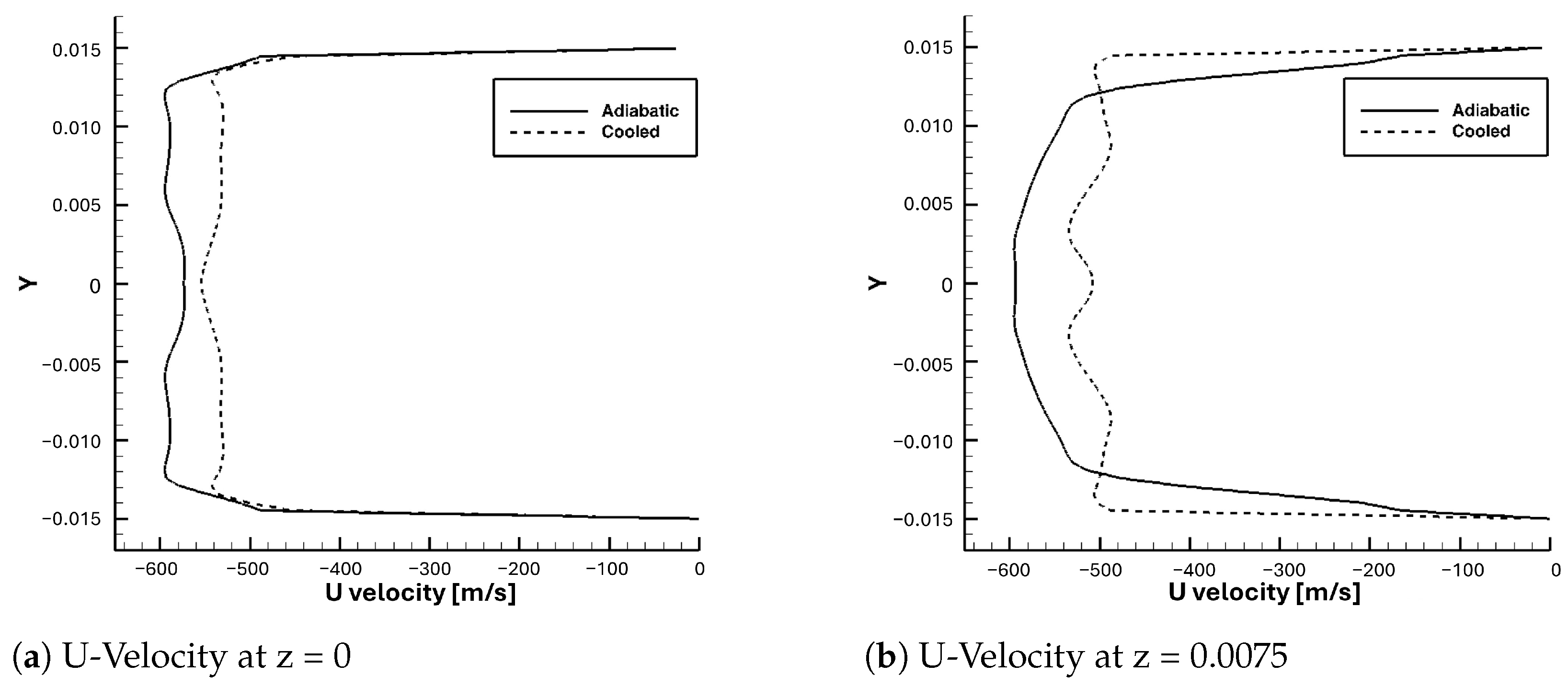
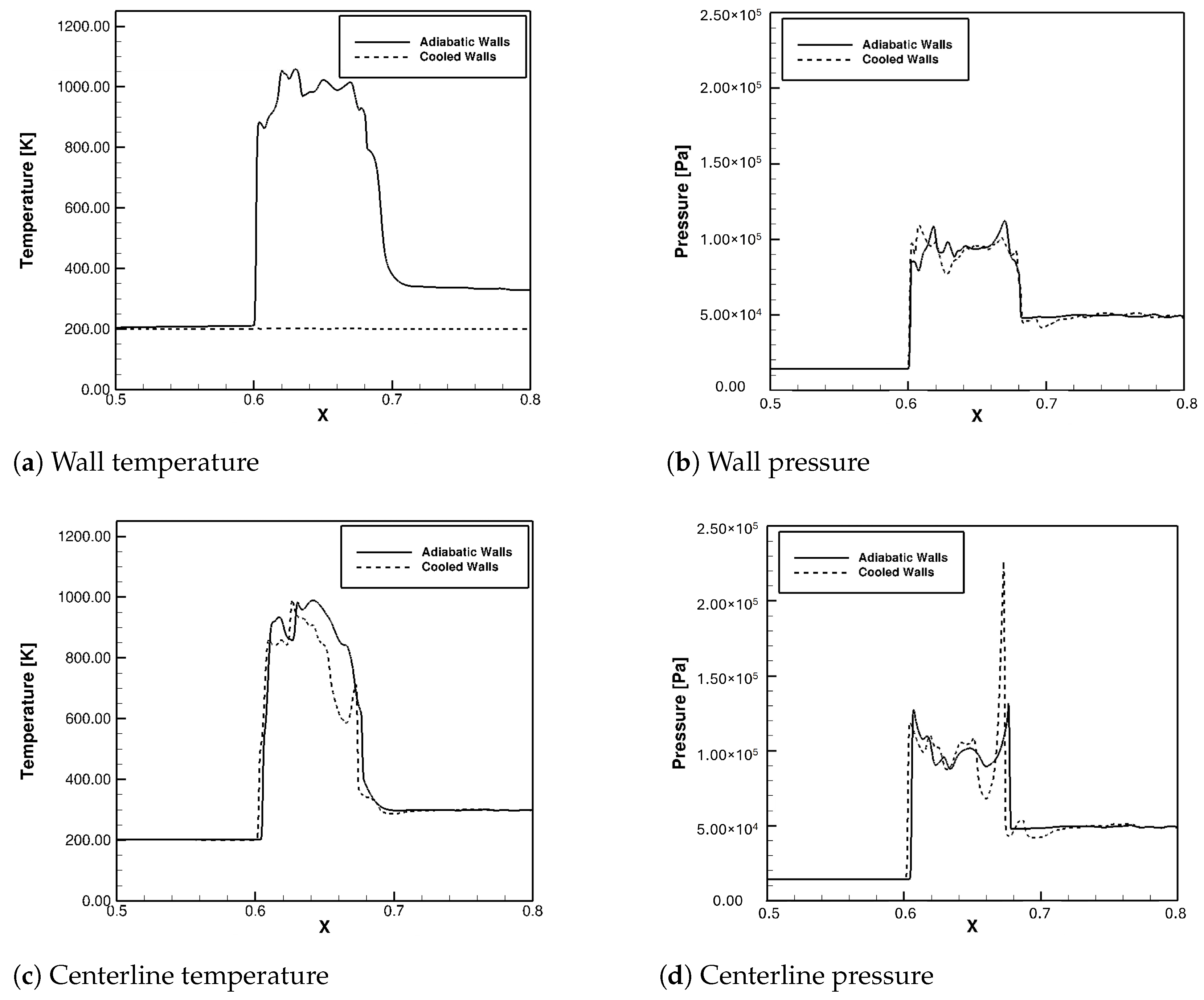
3.4. Effect of Wall Cooling
4. Shock Interference in Modified Shock-Tube
4.1. Mesh
4.2. Numerical Methods
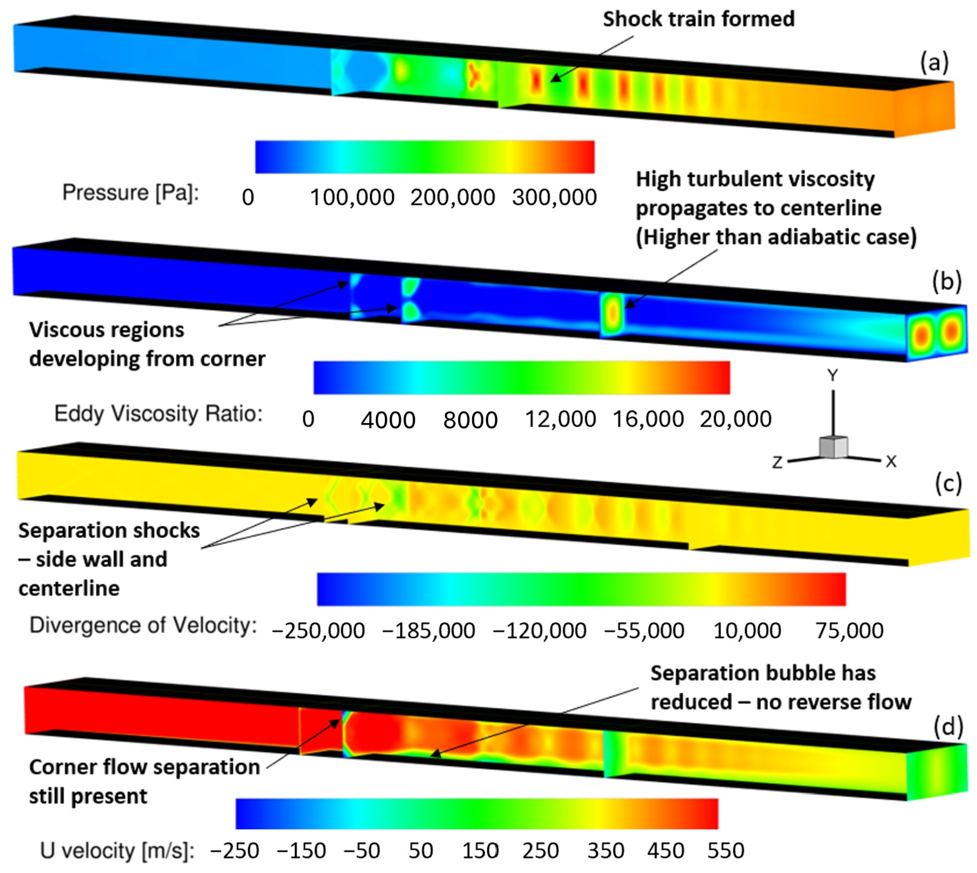
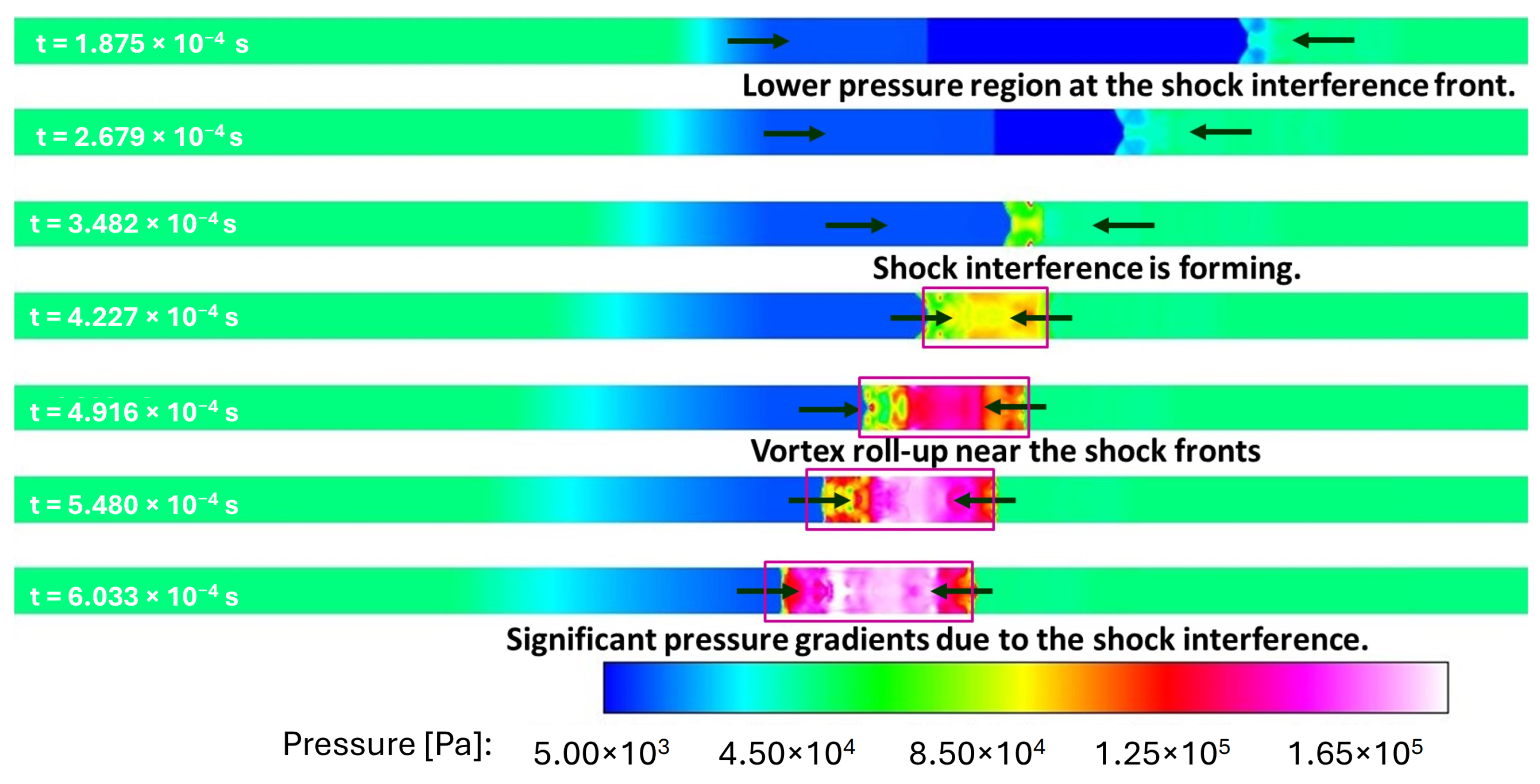
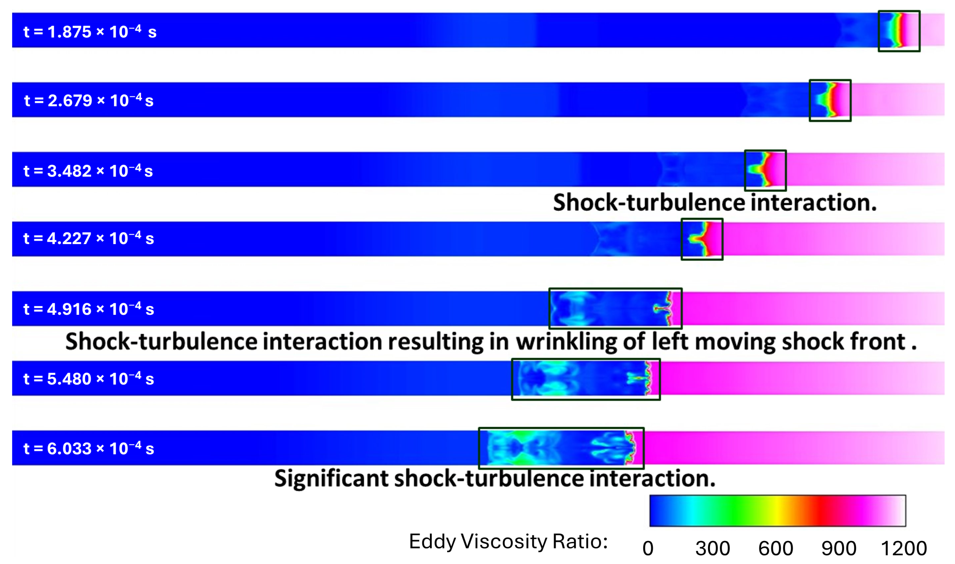
4.3. Results
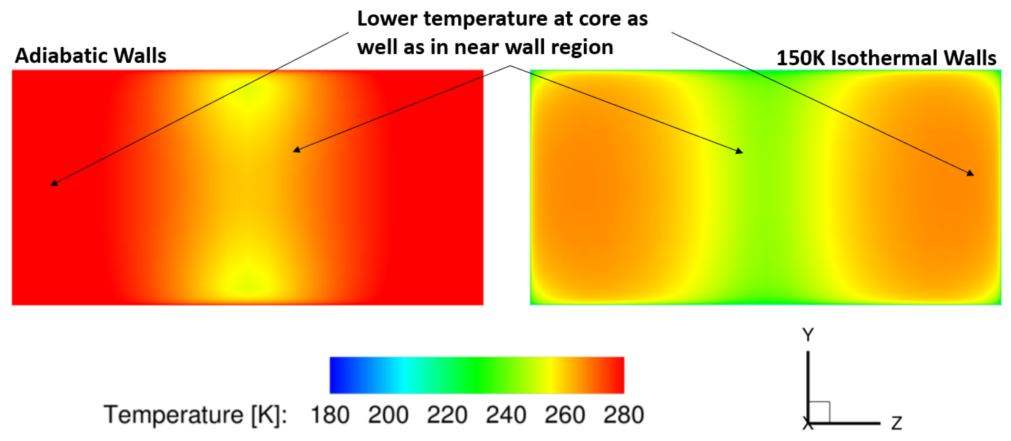
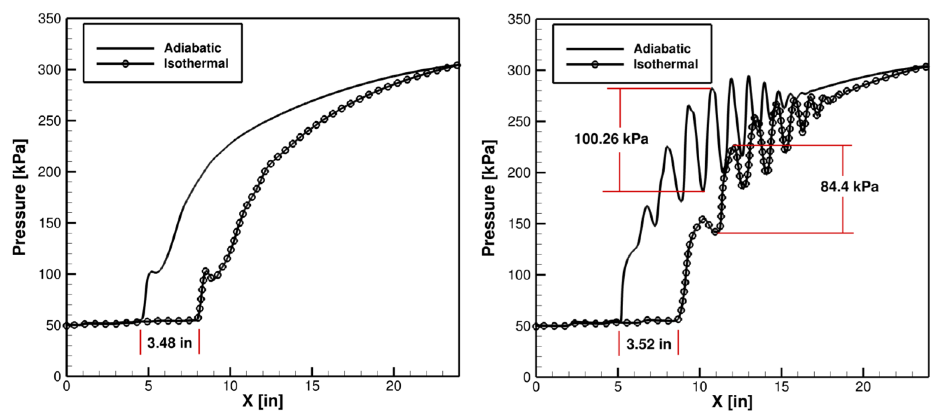
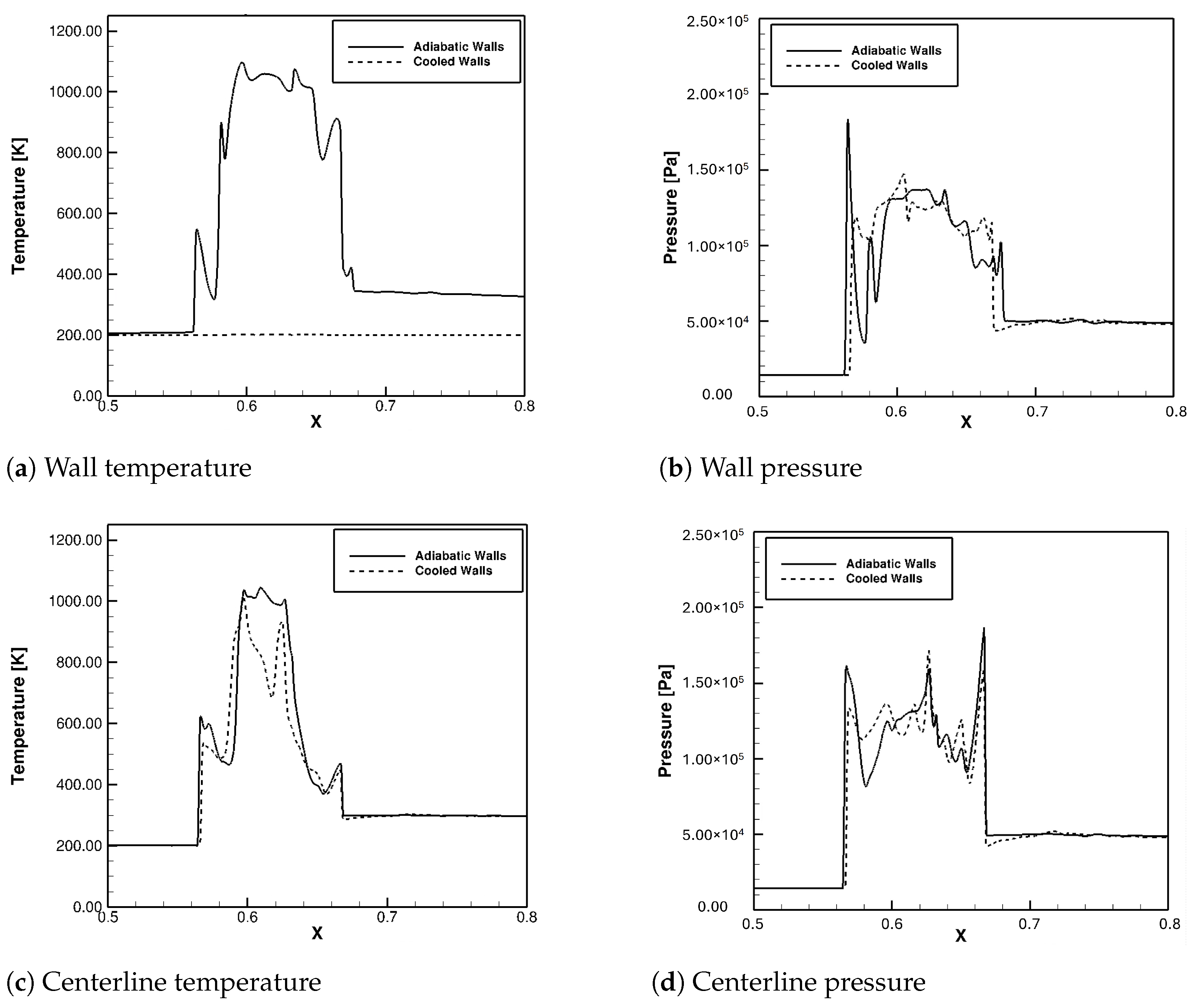
4.4. Effect of Wall Temperature on Shock Interference
5. Conclusions
Author Contributions
Funding
Institutional Review Board Statement
Informed Consent Statement
Data Availability Statement
Acknowledgments
Conflicts of Interest
References
- Heiser, W.H.; Pratt, D.T. (Eds.) Hypersonic Airbreathing Propulsion; AIAA Education Series; AIAA: New York, NY, USA, 1994. [Google Scholar]
- Curran, E.T. Scramjet Engines: The First Forty Years. J. Propuls. Power 2001, 17, 1138–1148. [Google Scholar] [CrossRef]
- Waltrup, P.; White, M.E.; Zarlingo, F.; Gravlin, E.S. History of U.S. Navy Ramjet, Scramjet, and Mixed-Cycle Propulsion Development. J. Propuls. Power 2002, 18, 14–27. [Google Scholar] [CrossRef]
- Fry, R.S. A Century of Ramjet Propulsion Technology Evolution. J. Propuls. Power 2004, 20, 27–58. [Google Scholar] [CrossRef]
- Do, H.; Im, S.-K.; Mungal, M.G.; Cappelli, M.A. The influence of boundary layers on supersonic inlet flow unstart induced by mass injection. Exp. Fluids 2011, 51, 679–691. [Google Scholar] [CrossRef]
- Rodi, P.E.; Emami, S.; Trexler, C.A. Unsteady Pressure Behavior in a Ramjet/Scramjet Inlet. J. Propuls. Power 1996, 12, 486–493. [Google Scholar] [CrossRef]
- Carroll, B.; Dutton, J.C. Turbulence Phenomena in a Multiple Normal Shock Wave/Turbulent Boundary-Layer Interaction. AIAA J. 1992, 30, 43–48. [Google Scholar] [CrossRef]
- Acharya, R.; Palies, P.; Schetz, J.; Schmisseur, J. Development of Uncertainty Quantification Framework Applied to Scramjet Unstart Challenge. In Proceedings of the 23rd AIAA International Space Planes and Hypersonic Systems and Technologies Conference, Montreal, QC, Canada, 10–12 March 2020. [Google Scholar] [CrossRef]
- Acharya, R.; Schetz, J.; Schmisseur, J.D. Non-Intrusive Computational Method and Uncertainty Quantification for Isolator Operability Calculations: Part 1. In Proceedings of the 2018 Joint Propulsion Conference, Cincinnati, OH, USA, 9–11 July 2018. [Google Scholar] [CrossRef]
- Acharya, R. Identification and Assessment of Scramjet Isolator Unstart and Operability Metrics. Aerospace 2025, 12, 503. [Google Scholar] [CrossRef]
- Weiting, A. Multiple shock-shock interference on a cylindrical leading edge. AIAA J. 1992, 30, 2073. [Google Scholar] [CrossRef]
- Boldyrev, S.M.; Borovoy, V.Y.; Chinilov, A.Y.; Gusev, V.N.; Krutiy, S.N.; Struminskaya, I.V.; Yakovleva, L.V.; Délery, J.; Chanetz, B. A thorough experimental investigation of shock/shock interferences in high Mach number flows. Aerosp. Sci. Technol. 2001, 5, 167–178. [Google Scholar] [CrossRef]
- Grasso, F.; Purpura, C.; Chanetz, B.; Délery, J. Type III and type IV shock/shock interferences: Theoretical and experimental aspects. Aerosp. Sci. Technol. 2003, 7, 93–106. [Google Scholar] [CrossRef]
- Cardona, V.; Joussot, R.; Lago, V. Shock/shock interferences in a supersonic rarefied flow: Experimental investigation. Exp. Fluids 2021, 62, 135. [Google Scholar] [CrossRef]
- Edney, B. Anomalous Heat Transfer and Pressure Distributions on Blunt Bodies at Hypersonic Speeds in the Presence of an Impinging Shock. FFA Report 115; 1968. Available online: https://www.osti.gov/biblio/4480948 (accessed on 24 May 2025).
- Valdivia, A.; Yuceil, K.B.; Wagner, J.L.; Clemens, N.T.; Dolling, D.S. Control of Supersonic Inlet-Isolator Unstart Using Active and Passive Vortex Generators. AIAA J. 2014, 52, 1207–1218. [Google Scholar] [CrossRef]
- Sethuraman, V.R.P.; Kim, T.H.; Kim, H.D. Control of the oscillations of shock train using boundary layer suction. Aerosp. Sci. Technol. 2021, 118, 1872–1873. [Google Scholar] [CrossRef]
- Sethuraman, V.R.P.; Yang, Y.; Kim, J.G. Low-frequency shock train oscillation control in a constant area duct. Phys. Fluids 2022, 34, 016105. [Google Scholar] [CrossRef]
- NASA LaRC. Turbulence Modeling Resource. Available online: https://turbmodels.larc.nasa.gov/ (accessed on 29 June 2025).
- Harris, N.; Stokes, T.M.; Acharya, R. A Comparison of Turbulence Models for Scramjet Isolator Unstart Estimation. In Proceedings of the AIAA SCITECH 2023 Forum, National Harbor, MD, USA, 23–27 January 2023; p. 0711. [Google Scholar]
- Toro, E. Riemann Solvers and Numerical Methods for Fluid Dynamics: A Practical Introduction; Springer: Berlin/Heidelberg, Germany, 2014. [Google Scholar]
- Baurle, R.A.; Middleton, T.F.; Wilson, L.G. Reynolds-Averaged Turbulence Model Assessment for a Highly Back-Pressured Isolator Flowfield. In Proceedings of the 33rd Airbreathing Propulsion Joint Subcommittee Meeting, Atlanta, GA, USA, 30 July–1 August 2012. [Google Scholar]
- Wilcox, D.C. Comparison of two-equation turbulence models for boundary layers with pressure gradient. AIAA J. 1993, 31, 1414–1421. [Google Scholar] [CrossRef]
- Deardorff, J.W. A numerical study of three-dimensional turbulent channel flow at large Reynolds numbers. J. Fluid Mech. 1970, 41, 453–480. [Google Scholar] [CrossRef]
- Van Leer, B. Towards the ultimate conservative difference scheme. V. A second-order sequel to Godunov’s method. J. Comput. Phys. 1979, 32, 101–136. [Google Scholar] [CrossRef]
- Sutherland, W. LII. The viscosity of gases and molecular force. Lond. Edinb. Dublin Philos. Mag. J. Sci. 1893, 36, 507–531. [Google Scholar] [CrossRef]
- Smagorinsky, J. General Circulation Experiments with the Primitive Equations. Mon. Weather. Rev. 1963, 91, 99. [Google Scholar] [CrossRef]
- Alexander, C.; Acharya, R. Computational Investigations of Shock Interference in a Scramjet Isolator. In Proceedings of the AIAA Aviation Forum and Ascend 2024, Las Vegas, NV, USA, 29 July–2 August 2024. [Google Scholar]


| Baurle et al. [22] | Current Work | |
|---|---|---|
| Dimensions | 24 × 0.5 × 1 [in] | 0.6096 × 0.0127 × 0.0254 [m] |
| Mesh (Isolator) | ||
| Points | 2000 × 160 × 208 * 1000 × 80 × 104 | 1000 × 80 × 104 |
| Max. y+ | 1.0 | 1.0 |
| Streamwise spacing in first half of isolator | 0.01 h | 0.02 h |
| Streamwise spacing in second half of isolator | 0.01 h → 0.025 h | 0.02 h → 0.025 h |
| Max. grid spacing in vertical and spanwise directions | 0.01 h | 0.02 h |
| Solution Methodology | ||
| Numerics scheme | Incomplete LU | Incomplete LU |
| CFL number | 100 | 100 |
| Flux scheme | LDFSS | LDFSS |
| Flow variable reconstruction scheme | MUSCL, k = | MUSCL, k = |
| Flux limiter | Koren | Koren |
| Model Specifications | ||
| Turbulence Model | Wilcox 1998 | Wilcox 1998 |
| Molecular and Turbulent Pr | 0.72, 0.9 | 0.72, 0.9 |
| Viscosity model | McBride | Sutherland’s Law |
| Baurle et al. [22] | Current Work | |
|---|---|---|
| Total Temperature at Entry [K] | 292.91 | 297.90 |
| Nozzle Plenum Pressure or Isentropic Total Pressure [kPa] | 845.29 | 845.29 |
| Isolator Entry Pressure [kPa] | 49.47 | 49.47 |
| Isolator Back Pressure [kPa] | 304.51 | 304.51 |
| Pressure Ratio | 0.360 | 0.360 |
| Baurle et al. [22] | Current Work | |
|---|---|---|
| Shock-train Length (top-wall centerline) | 8.62 inches | 10.00 inches |
Disclaimer/Publisher’s Note: The statements, opinions and data contained in all publications are solely those of the individual author(s) and contributor(s) and not of MDPI and/or the editor(s). MDPI and/or the editor(s) disclaim responsibility for any injury to people or property resulting from any ideas, methods, instructions or products referred to in the content. |
© 2025 by the authors. Licensee MDPI, Basel, Switzerland. This article is an open access article distributed under the terms and conditions of the Creative Commons Attribution (CC BY) license (https://creativecommons.org/licenses/by/4.0/).
Share and Cite
Alexander, C.; Acharya, R. Computational Investigations and Control of Shock Interference. Appl. Sci. 2025, 15, 7963. https://doi.org/10.3390/app15147963
Alexander C, Acharya R. Computational Investigations and Control of Shock Interference. Applied Sciences. 2025; 15(14):7963. https://doi.org/10.3390/app15147963
Chicago/Turabian StyleAlexander, Cameron, and Ragini Acharya. 2025. "Computational Investigations and Control of Shock Interference" Applied Sciences 15, no. 14: 7963. https://doi.org/10.3390/app15147963
APA StyleAlexander, C., & Acharya, R. (2025). Computational Investigations and Control of Shock Interference. Applied Sciences, 15(14), 7963. https://doi.org/10.3390/app15147963