Application of Deep Neural Networks in Recognition of Selected Types of Objects in Digital Images

Abstract

The presented article focuses on the application of deep neural networks for recognizing selected types of objects in digital images. Various learning techniques, network architectures, and hyperparameters were analyzed to optimize the detection quality. This study compared supervised learning, self-supervised learning, and transfer learning methods, with YOLOv8 showing the highest effectiveness in the transfer learning approach. This article is of a typical application nature. The results included in it can be used by a potential reader for other applications related to object recognition in digital images.

1. Introduction

Artificial intelligence is a rapidly developing IT direction. Nowadays, it is becoming an inseparable part of human needs and conveniences. The constant demand for more and more abstract automations causes an increase in supply from corporations providing software—currently, most often in the form of software based on artificial intelligence algorithms. With each subsequent year of development, this area covers more and more areas of modern life. Today, AI is used, among others, in medicine, automotive, mobile devices, tourism, or agriculture. Good examples include airport baggage checks [1], facial recognition [2], handwriting recognition [3], stock market forecasts [4], and even weather forecasts [5].

There are many possibilities of creating or using an already trained model based on machine learning algorithms. However, the use of different learning techniques, different network architectures, and the appropriate selection of parameters may turn out to be different depending on the type of data that our algorithm is supposed to process. For example, to create a model that is supposed to process digital images and classify objects on it, it will be beneficial to use, among others, convolutional networks (CNNs), because these networks allow for the detection of increasingly complex patterns and features in the input data. Thanks to the use of a structure inspired by the biological visual cortex, convolutional networks can effectively analyze images by gradually processing information on successive layers, which leads to a reduction in the number of parameters and improved efficiency compared to traditional neural networks [6]. Another example is natural language processing and the process of generating new text based on existing text data or templates. In this case, the approach based on recurrent neural networks (RNNs) is popular, because their architecture allows for processing sequential data and learning the relationships between these sequences [7,8]. Although convolutional networks are currently mainly used for detecting objects in digital images, there are still different approaches that can be used in this aspect. For example, when creating a model, different architectures, numbers of layers and parameters are used, which can be adapted to a specific task. Some approaches will generate better results in terms of precision, accuracy, and sensitivity, but require more time to train the model or the matching process. Other approaches are faster, but may lead to worse results.

New architectures are constantly being developed, which are characterized by increasing accuracy of the work performed. From 2010 to 2017, annual competitions were held for classification of 2D objects from the ImageNet database [9]. To win, the neutral network had to achieve the lowest possible error level during classification of test data. The AlexNet and GoogLeNet architectures discussed in this paper won in 2012 and 2014 [10], respectively. In the case of detecting objects in digital images, different techniques are also used. One such approach is to combine convolutional networks with region proposal networks (RPNs). This approach can significantly speed up the learning and matching processes, because the image regions where the potential object is most likely to be located are checked [11]. Due to the existence of many possibilities for constructing an artificial intelligence model, questions may arise regarding the optimal selection of the network architecture and parameters for a given type of data and what may affect such a choice. In response to these and other questions, a research project was undertaken. An additional motivation to conduct the research presented below were three articles. The first article [12] focuses on defining the advantages and limitations of using a given machine learning technique. The work is a kind of comparative review of a large number of scientific works related to the machine learning techniques specified in the title. The selected techniques include self-supervised learning (SLE) and transfer learning (TLE). The authors provide guidelines for selecting the optimal technique for specific deep learning applications, aiming to solve the problem of data scarcity. According to the authors, the biggest advantage of transfer learning (TL) is the ability to train models based on simulations, which provides a controlled and safe environment for teaching the model to perform specific actions. In turn, the biggest advantage of self-supervised learning (SSL) is saving time on data labeling.

The next paper [13] focuses on the comparison of three architectures that are models of convolutional neural networks. The article aimed to show which of the three architectures mentioned in the title will guarantee the best results in terms of handwriting recognition accuracy and will provide the shortest time needed to classify data from the test set. The authors took care of the proper implementation of the models and training it on real data, which gave the work a research character.

The last work [14] is devoted to the development of a new Adaptive Hyperparameter Tuning (AHT) algorithm to automate the selection of optimal hyperparameters for convolutional neural network (CNN) models used in medical image classification. The authors focus on optimizing such hyperparameters as learning rate, epoch size, batch size, activation functions, and kernel/filter size. The Adaptive Hyperparameter Tuning algorithm uses the Gaussian process methodology and Parzen tree estimator to evaluate different combinations of hyperparameters and selects the ones that provide the highest model accuracy. The hyperparameter optimization was performed on a medical dataset that was used to validate the classification of malignant and benign tumors.

The presented project includes the implementation, which is a number of different approaches to constructing an artificial intelligence model using deep neural networks to recognize selected types of objects in digital images. The research also includes a comparison of the quality indicators of matches of the network created from scratch with the results of object detection using a pre-trained YOLO (You Only Look Once) model. The aim of the work is to analyze the obtained results and draw appropriate conclusions regarding the impact of the selection of a given parameter or approach on the obtained results. The planned experiments also include an evaluation of the performance of various deep neural network architectures to identify optimal approaches to recognizing objects in images. In addition to analyzing the effectiveness of object detection, the project also involves examining the performance of the created models in terms of processing time and system resource consumption, which is crucial for their practical implementation.

The genesis of the research presented in this article can be indicated as the lack in the literature, according to the best knowledge of the authors, of a comparison of three neural network models that belong to convolutional neural networks: LeNet-5, AlexNet, and GoogLeNet. Although these models are not the newest, they are still the subject of research [15,16,17,18]. This fact is also the reason for conducting the research presented in this article. In addition, the LeNet-5 model is mainly recommended for handwriting recognition, and in our approach, it was used for animal recognition in digital images. Due to its low complexity, it can also be considered for use in embedded systems with lower computing power than computing clusters. The article is of a typical application nature. The results included in it can be used by a potential reader for other applications related to object recognition in digital images. In our opinion, the literature lacks a comparison of these three convolutional neural network models, and in the currently very rapid development of neural network applications, it can be a very useful source of knowledge.

2. Results of Research

This section of the work focuses on an in-depth analysis of the results of studies that have been carried out to optimize neural network models and examine the effectiveness of various machine learning techniques. Special attention was paid to both classical supervised learning methods and modern approaches, such as self-supervised learning using the advanced SimSiam technique [19] and transfer learning [20], where the YOLOv8 model [21] is used. The first subsection will provide a detailed description of the research methods used, which formed the basis for the experiments. In the following subsections, the results of the experiments will be discussed in detail, with emphasis on the selection and impact of various hyperparameters, such as batch size, activation functions, and optimizers [22,23,24]. This analysis will identify the best parameter configurations that significantly affect the performance and efficiency of the models. In addition, a comparison of different neural network architectures, including LeNet5, AlexNet, and GoogLeNet, will be conducted to assess their ability to solve complex problems in the context of the research task.

Supervised learning, the cornerstone of classical approaches in machine learning, will be contrasted with more advanced methods such as self-supervised learning and transfer learning. Self-supervised learning [25,26] using the SimSiam technique will be described in detail, including its advantages and limitations compared to traditional methods. Transfer learning, using the YOLOv8 model, will be discussed in the context of its ability to adapt knowledge from other fields to specific research tasks. Each of these subsections will include an in-depth analysis of the results obtained and a discussion of their relevance in the context of building effective and efficient artificial intelligence models. Possible interpretations of the results will also be discussed, providing a better understanding of which approaches and parameter configurations are critical to success in specific tasks. This chapter will conclude with conclusions that summarize the most important insights from the research. There will also be suggestions for potential directions for further research that can further develop and improve machine learning methods and optimization of neural network models in various application contexts.

2.1. Description of Selected Convolutional Network Structures

LeNet-5

LeNet-5 is a classic convolutional neural network architecture, proposed by Yann LeCun in 1998. It was created mainly for recognizing handwritten digits, which has been used in banking for automatic check reading [27].

LeNet-5 consists of seven layers, which include convolutional layers, subsampling layers, and fully connected layers. The specific structure shown in Figure 1 is as follows:

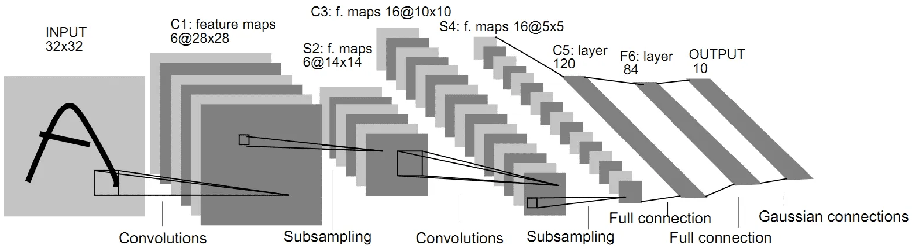
• Two convolutional layers: the first one processes the input image of 32 × 32 pixels, using 6 filters of size 5 × 5 pixels. The second convolutional layer uses 16 filters.
• Two subsampling layers: they reduce the resolution of feature maps using max-pooling operations.
• Three fully connected layers: these layers function similarly to the classical multilayer perceptron layers and are used for final classification [27].

LeNet-5 was chosen for this study for several reasons. First of all, it is a relatively low-computational-cost architecture, which makes it suitable for preliminary experiments and as a starting point for more advanced models. Furthermore, LeNet-5 is characterized by acceptable accuracy in classification tasks, which is crucial when computational resources are limited.

AlexNet

The AlexNet architecture was designed by Alex Krizhevsky, Illy Sutskever, and Geoffrey Hinton in 2012. It is one of the first deep neural networks that gained wide recognition in the field of computer vision. AlexNet consists of eight layers, which include convolutional layers, max-pooling layers, and fully connected layers [29].

The specific structure shown in Figure 2 is as follows:

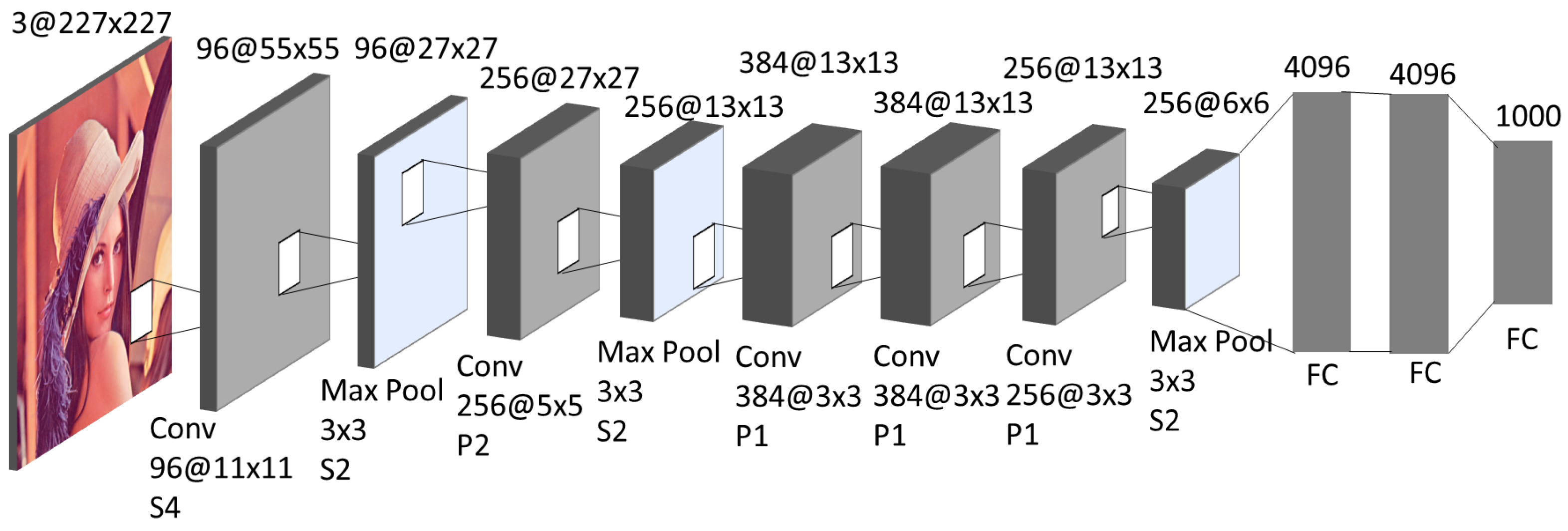
• Five convolutional layers: the first convolutional layer processes the input image of 227 × 227 pixels (some sources use 224 × 224 pixels), using 96 filters of 11 × 11 pixels. The next convolutional layers apply smaller filters, 5 × 5 and 3 × 3, respectively, with different numbers of filters (256, 384, 384, 256).
• Three max-pooling layers: these layers reduce the resolution of the feature maps using max-pooling operations, which reduces the amount of data to be processed and introduces some robustness to image shifts.
• Three fully-connected layers: the first two fully-connected layers have 4096 neurons each and function similarly to classical multilayer perceptron layers, and the third fully-connected layer contains 1000 neurons and is used for final classification using the softmax function [29].

The choice of AlexNet for this study is due to its relatively simpler architecture compared to more complex models. AlexNet is a less complex architecture that falls between the simpler LeNet-5 and the more advanced GoogLeNet. AlexNet potentially combines the advantages of the less complex LeNet-5 architecture, such as lower computational requirements and faster training time, with the advantages of the more complex GoogLeNet, such as the ability to process and classify complex patterns in images. Additionally, it requires images of 227 × 227 pixels. For the images used in the study, which are in RGB format and have a size of approximately 300 × 200 pixels, only minimal rescaling is necessary. This avoids losing important information from the images.

GoogLeNet

GoogLeNet is an advanced convolutional neural network architecture developed by Google’s research team. This architecture has been successfully applied to many image processing tasks [31].

GoogLeNet consists of 22 layers, which include convolutional layers, reduction layers, and special modules called inception modules. The inception module is a key element of this architecture, which allows for efficient combination of information from different spatial scales [31]. The specific structure is shown in Figure 3.

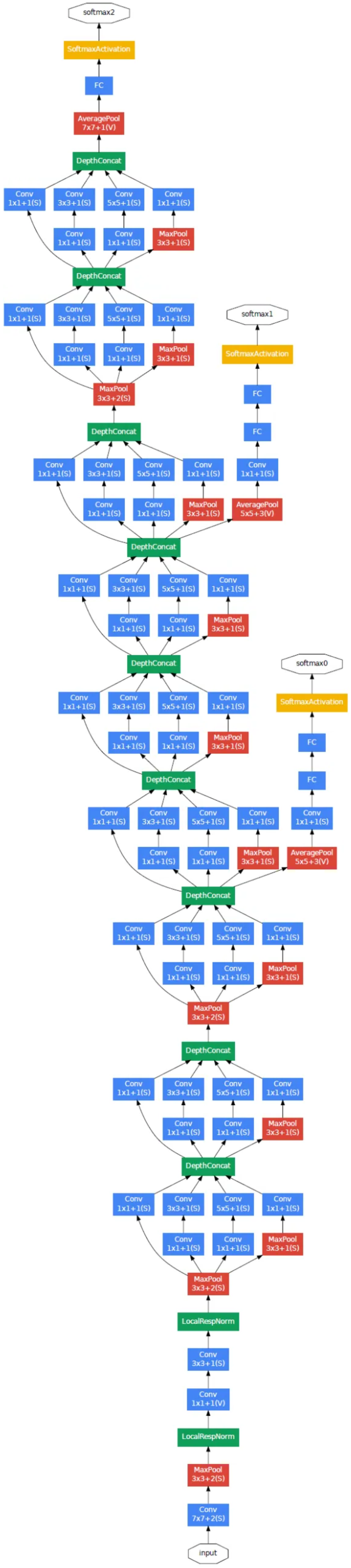
• Initial layers: The architecture starts with convolutional layers, which are used to extract features from the input image. Given a 224 × 224 × 3 input, the following operations are applied:

  –

  7 × 7 convolutional layer with 64 filters, stride 2, ReLU activation function;

  –

  MaxPooling2D layer with 3 × 3 filter size and stride 2;

  –

  1 × 1 convolutional layer with 64 filters, ReLU activation function;

  –

  3 × 3 convolutional layer with 192 filters, ReLU activation function;

  –

  MaxPooling2D layer with 3 × 3 filter size and stride 2.

• Nine inception modules (red boxes): Inception modules are the key element of the architecture, using multiple convolution branches with different filter sizes to efficiently extract features from images.
• Two softmax auxiliary layers (green boxes): These layers play a key role in the network training and regularization process. Their presence is intended to speed up the learning process by guiding the network towards the goal and ensuring that the intermediate functions generated by the network are good enough.
• Global Average Pooling: Instead of a fully connected layer, global averaging is used, which makes it easier to adjust and improve the network.

Softmax auxiliary layer structure:

• An averaging layer with a filter size of 5 × 5 and stride 3, giving an output of size 4 × 4 × 512 for the first auxiliary layer softmax0 and 4 × 4 × 528 for the second auxiliary layer softmax1;
• A 1 × 1 convolutional layer with 128 filters, with a ReLU function after each of them;
• A fully connected layer with 1024 neurons and a ReLU activation function;
• A dropout layer with a value of 70%;
• A linear layer with 1000 classes and a softmax function.

The inception module is a set of parallel convolutional and pooling operations that allow for feature extraction at different abstraction levels simultaneously. Within one module, convolutional operations with filters of sizes 1 × 1, 3 × 3, and 5 × 5 and max-pooling operation are used. The results of these operations are then combined along the channel dimension, which allows for reducing the number of parameters and the depth of the network without losing important information.

GoogLeNet is the most complex of the selected architectures, which will allow us to compare how increasing the complexity of the architecture improves the results. It offers excellent results in detecting more complex objects in images, making it an ideal choice for research on the detection of image classes depending on the animal species. This architecture requires images of 224 × 224 pixels.

2.2. Research Methodology

The research methodology in this work is based on a consistent approach to designing and conducting experiments to optimize neural network models and evaluate the effectiveness of various machine learning techniques. This section discusses in detail the methods of data collection, processing, and analysis that were used to obtain reliable and valuable research results. The approach considered both classical supervised learning methods and modern techniques such as self-supervised learning and transfer learning.

The data used in the study included both input and output data. The input data were images from the Animals-10 collection, which contains images of ten different categories of animals: dog, cat, horse, spyder, butterfly, chicken, sheep, cow, squirrel, elephant [33]. This collection was divided into a more extensive training collection and a test collection, which also served a validation function. In the supervised learning and transfer learning approaches, the data were explicitly categorized at the model training stage. In self-supervised learning, on the other hand, all images were placed in a single folder, as this type of learning does not require categorization of the data. Only after initial training, the model was trained on a smaller, categorized dataset using transfer learning, and then tested on a test set, allowing validation of the results. The outputs consisted of various results, including the following:

-

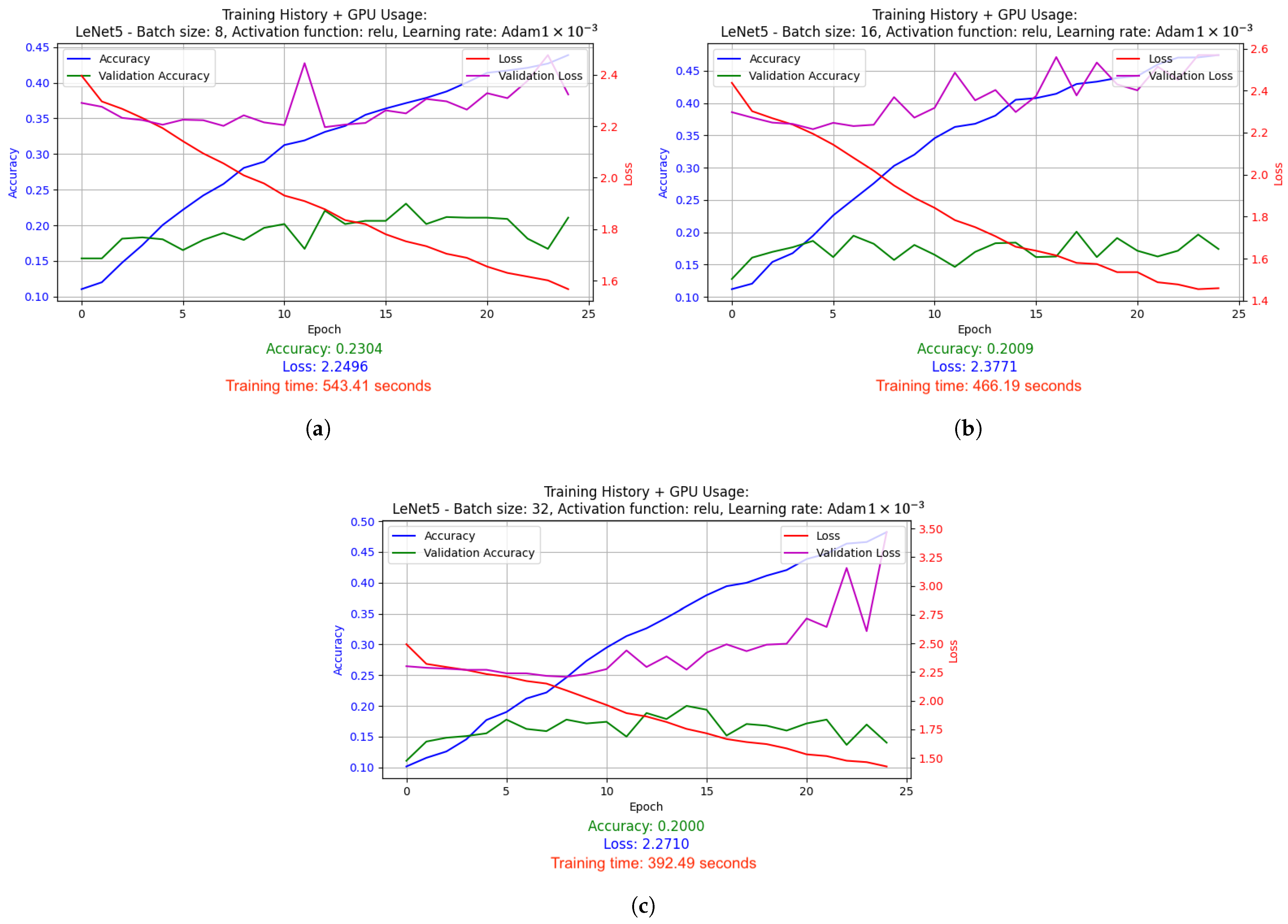
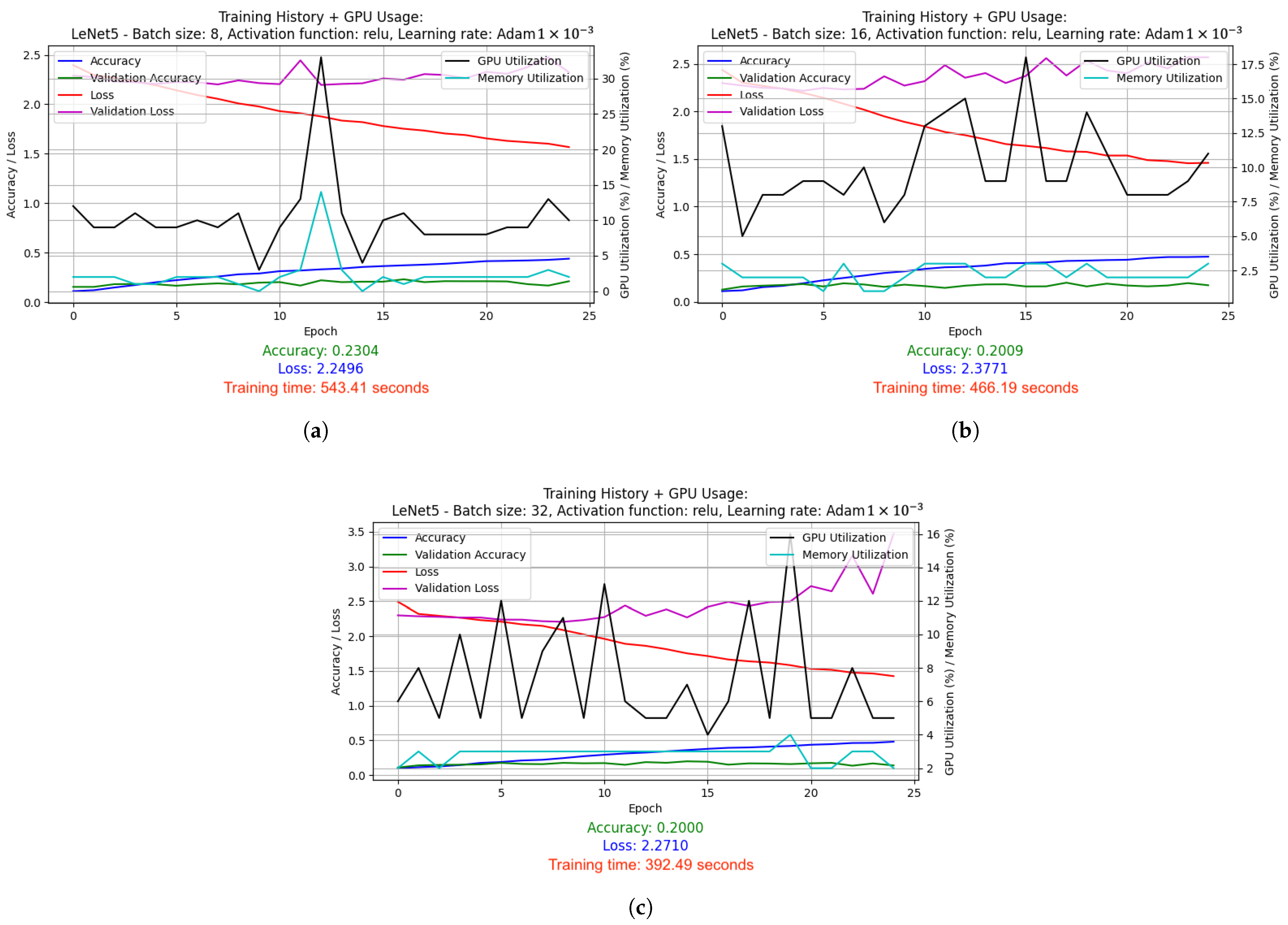
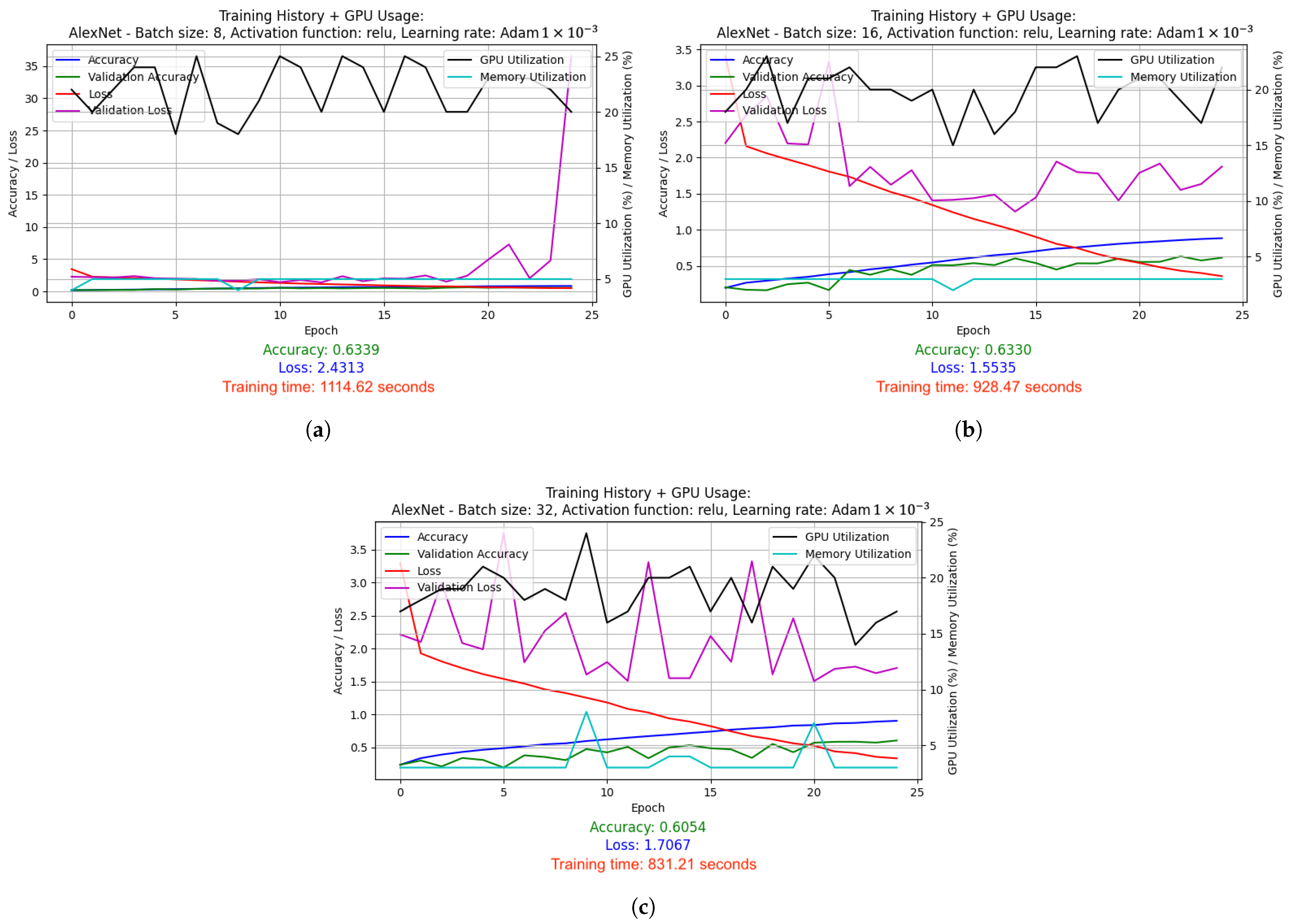
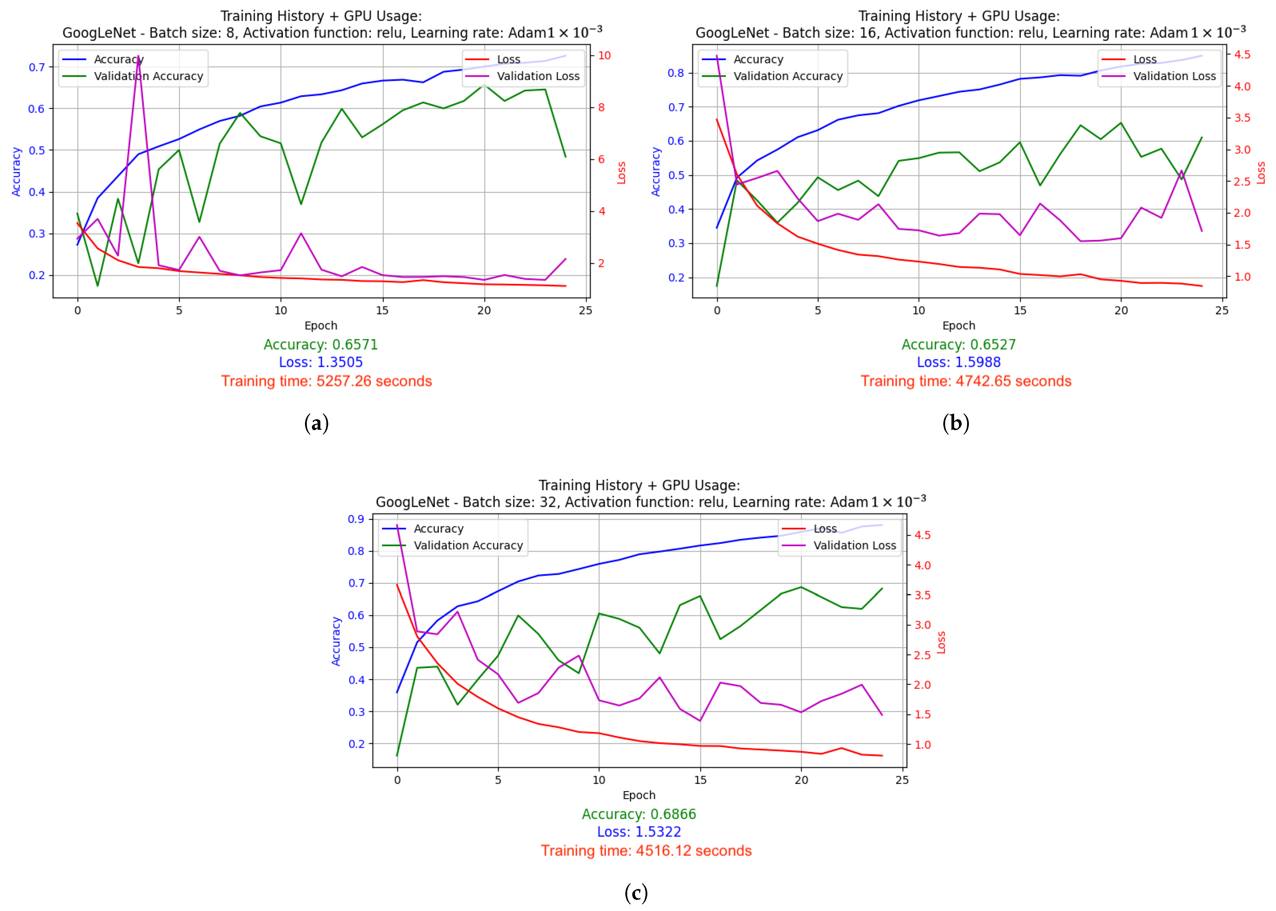
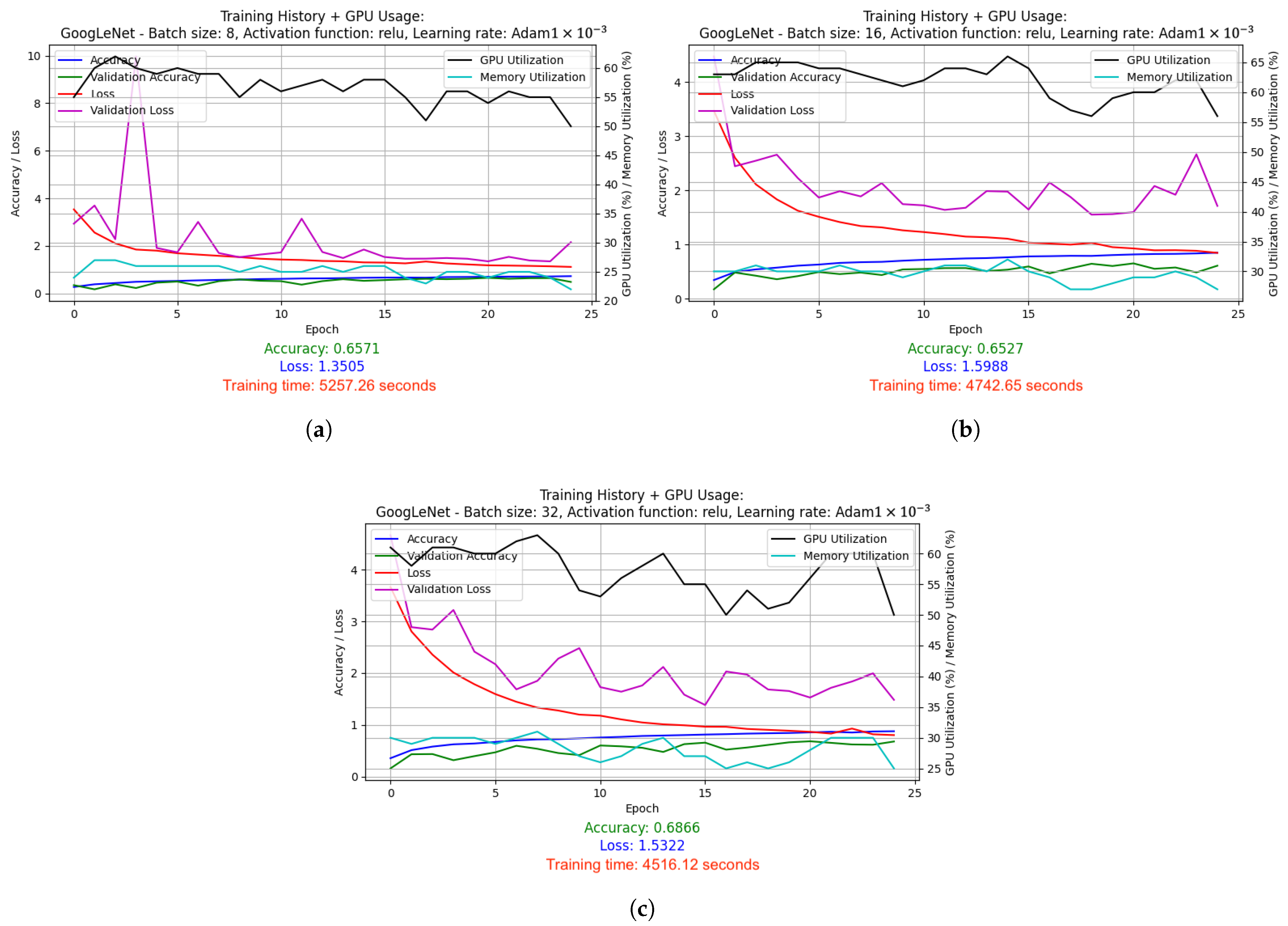
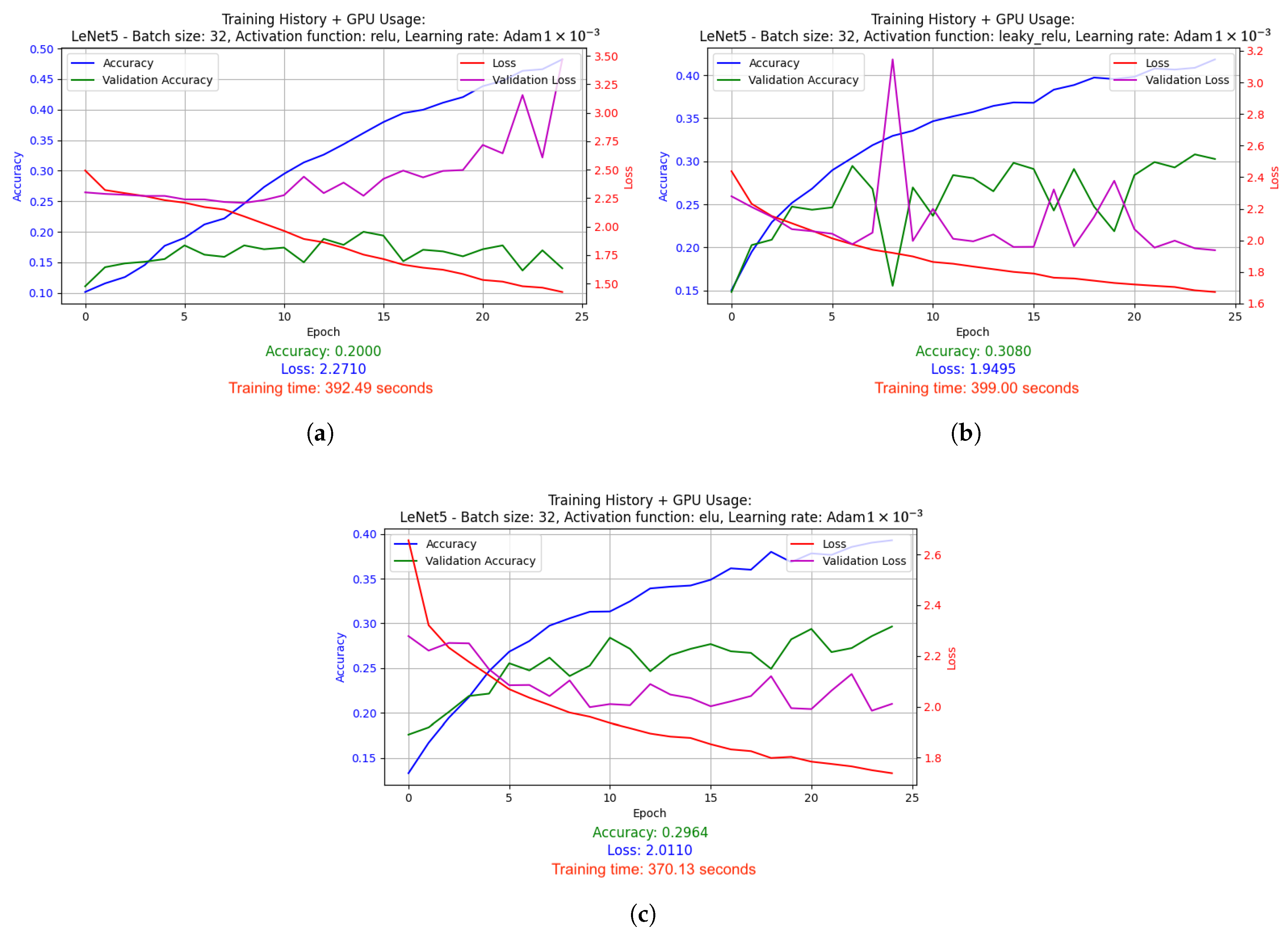
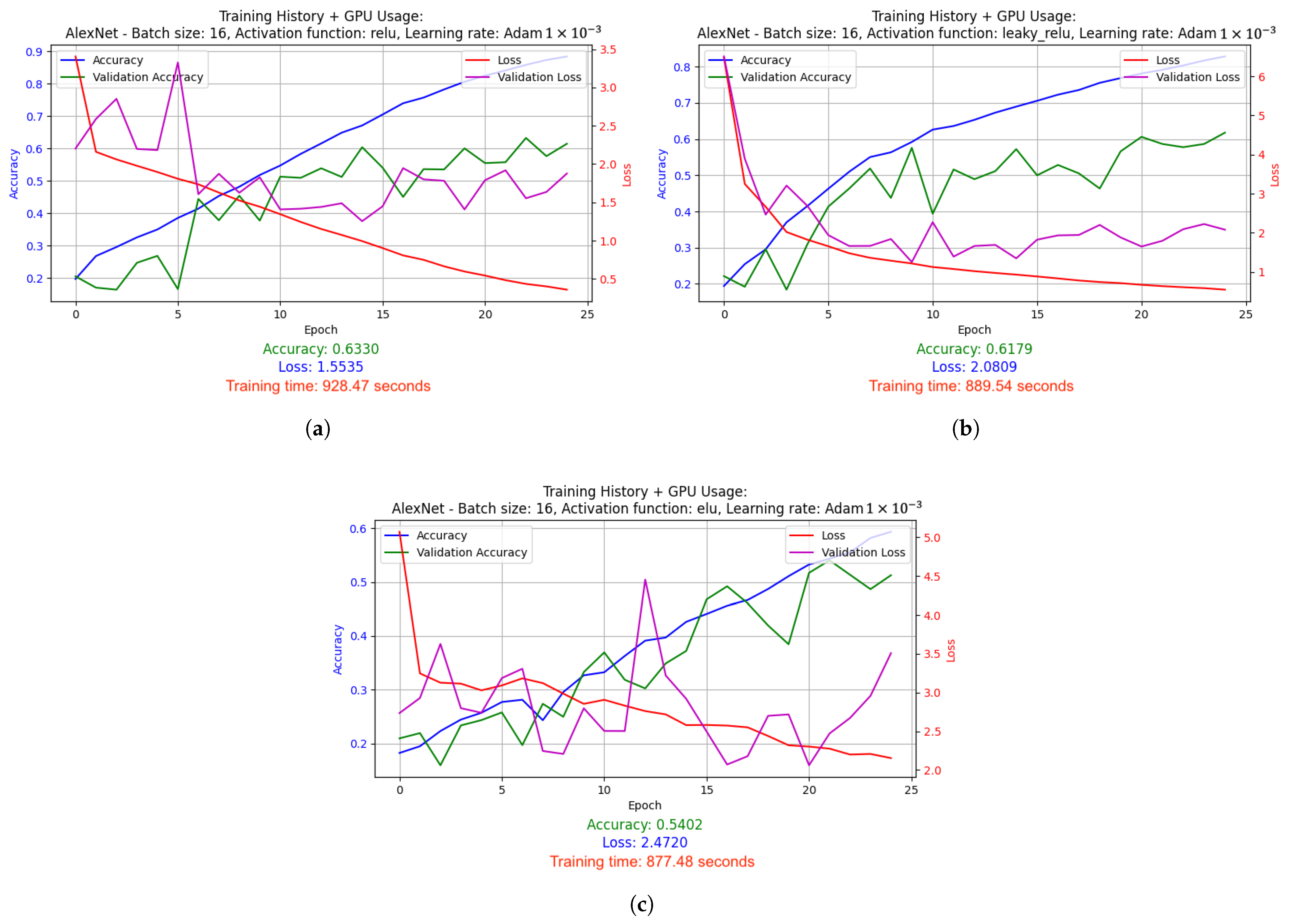
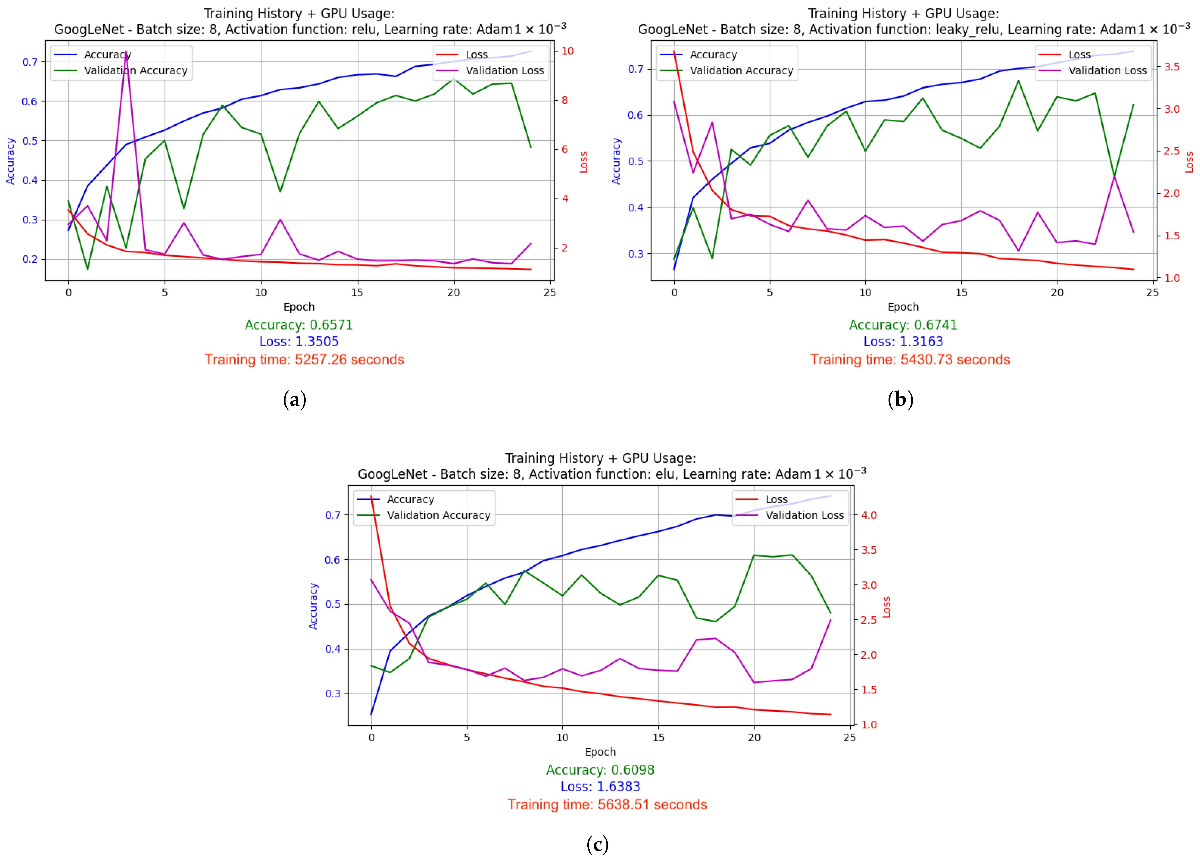
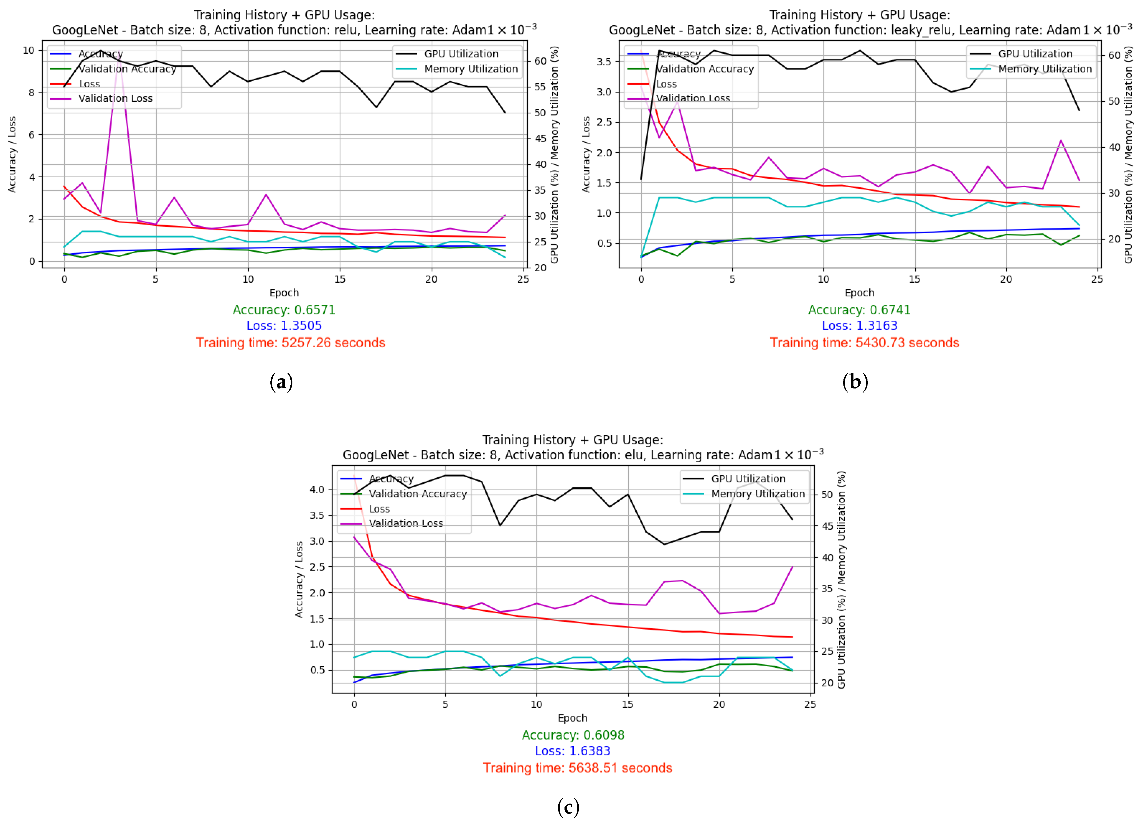
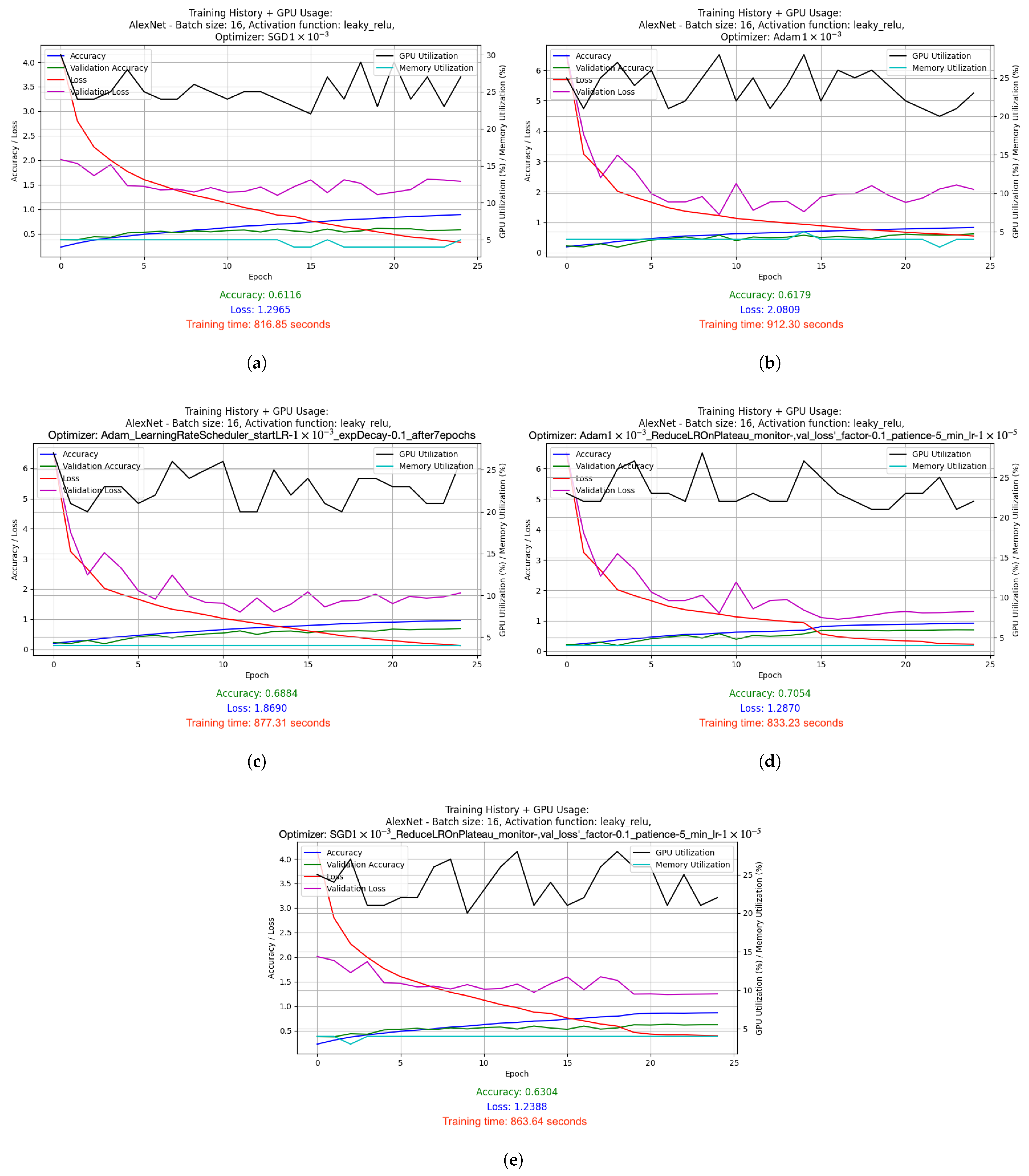
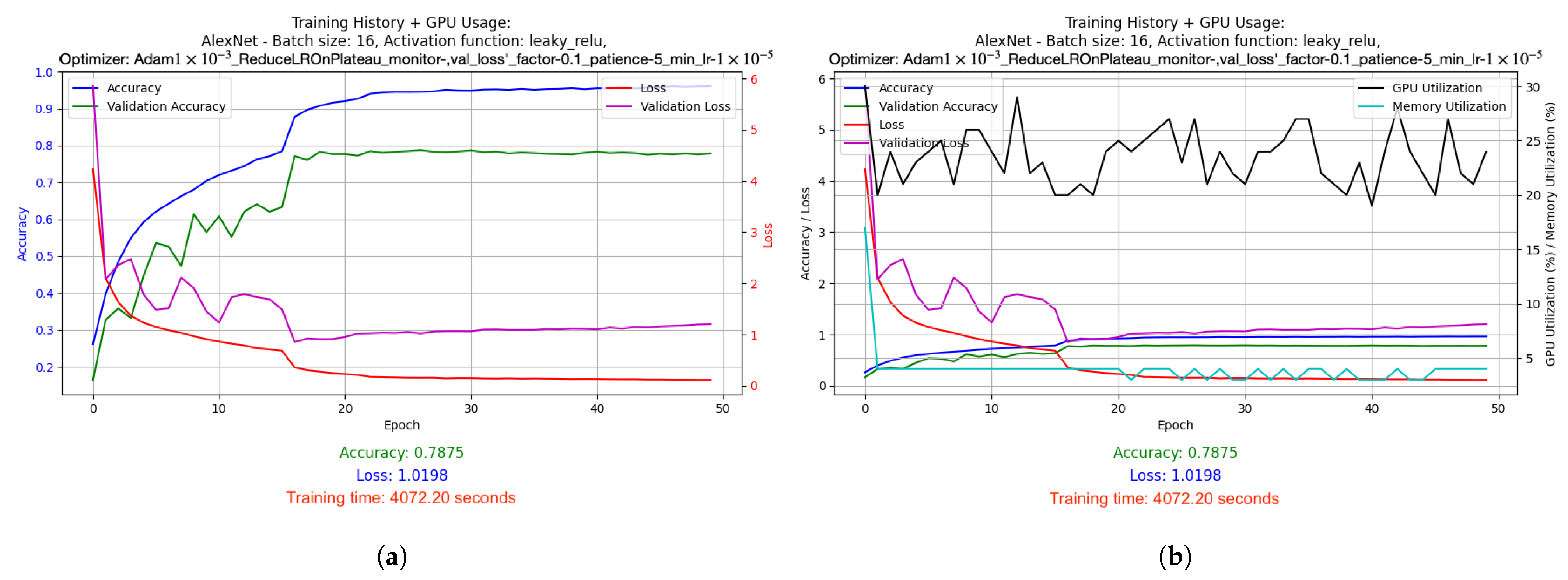
Graphs depicting the results of the conducted experiments. Two graphs were created for each experiment: a basic one, which included information such as accuracy, validation accuracy, loss and validation loss, and an extended version, which additionally showed GPU and memory usage.

-

Saved models after training, which can be used in the future for prediction or further testing.

-

Log files from TensorBoard and TensorFlow Profiler, which included training metrics such as accuracy and loss, as well as data on operation performance and resource consumption such as GPU and memory.

The sampling plan in this work addressed both the selection of appropriate data to train the models and the selection of hyperparameter values. In the case of imaging data, it was crucial to ensure that the training and test sets were representative so that models could be validated effectively. With regard to hyperparameters, an analysis of the literature and popular approaches was conducted to determine appropriate values. The study tested different batch sizes (8, 16, 32), activation functions (ReLU, Leaky ReLU, ELU) and optimizers with different learning rate settings [34]. The self-supervised learning approach used the best architecture from previous experiments (GoogLeNet) and the optimal batch size for best results.

Data collection in this project was conducted through scripts written in Python 3.13.5, which automated the process of training models and collecting results. For supervised learning, scripts were prepared for three architectures: LeNet5, AlexNet, and GoogLeNet. Each of these scripts allowed experimentation with different values of hyperparameters, which allowed a thorough analysis of the impact of these parameters on the effectiveness of the models. This study began by selecting the most popular approach, the ReLU activation function and the Adam optimizer with an initial learning rate of 1 × 10⁻³. Then, after determining the best batch size, subsequent experiments with the activation function used this best size, and only the activation function itself was changed. In the optimizer studies, once the optimal batch size and activation function were determined, only the choice of optimizer was already manipulated. For self-supervised learning, two scripts were created: one to perform training using the SimSiam architecture, and another to train the model with frozen weights. For the transfer learning approach, a single script was used to train the YOLOv8 model. To ensure fair results when selecting optimal hyperparameters in the first approach, a deterministic approach was used using seed. This ensured that the results were independent of randomness, allowing a more accurate comparison of different configurations and eliminating the influence of random factors on the experimental results. To maintain the reliability and consistency of the results, a learning length of 50 epochs was used in each approach. It should be noted, however, that in the case of the first approach, supervised learning, in order to select the best hyperparameters more quickly, training was initially carried out for 25 epochs, using part of the learning dataset. This allowed the initial selection of optimal hyperparameter settings in less time. Once the best configurations were selected, the model was already trained on the full dataset for 50 epochs, which allowed the final results to be obtained while saving a significant amount of time. The final results enabled the identification of the most efficient architecture.

2.3. Data Analysis Methods

Data analysis was mainly conducted using TensorFlow’s built-in mechanisms for tracking training history, which was then visualized using the Matplotlib 0.13.1 library. Callbacks were also used to monitor and respond to changes in metrics as models were trained. In addition, tools such as TensorBoard and TensorFlow Profiler allowed for more advanced visualization and monitoring of training metrics, such as accuracy and loss, and resource consumption (GPU, RAM, CPU). This made it possible to optimize models and compare the results of different configurations, allowing a thorough understanding of the impact of different hyperparameter settings on model performance. The time module was used to accurately measure training time, while the pynvml library allowed monitoring GPU resource consumption, which was crucial for optimizing computational processes when training deep neural networks.

2.4. Tools and Software

In the course of the research, a number of tools and software were used to support the process of training and analyzing the models, and special attention was required in terms of version compatibility. When working with advanced deep learning tools such as TensorFlow 1.2 and Keras 3, it is very important that all the libraries and tools used are compatible with each other. Many times, software versions are not fully compatible, leading to problems that can be time-consuming and labor-intensive to resolve. This process requires careful adjustment of tool versions to ensure a stable environment for model training. To optimize the performance of model training on the graphics card, CUDA and cuDNN were also used, which allowed for significant acceleration of computational processes. Thanks to their use, it was possible to significantly reduce the time required to train models, which is invaluable when working with large datasets and complex neural network architectures.

2.5. Test Results

2.5.1. Results of Hyperparameter Optimization Experiments for Supervised Learning Technique

This section presents the results of experiments on the selection of optimal hyperparameters, such as batch size, activation functions, and optimizers with different learning rate settings. In the first stage of the study, for the supervised learning approach, preliminary experiments were conducted with a limited number of epochs (25) and a partial dataset, which allowed rapid selection of the best hyperparameter configurations. Once the optimal values were selected, full model training was conducted on the full dataset for 50 epochs, ensuring reliable and comparable results. Formula (1) is used to evaluate the quality of the models from the first approach, which was used to optimize the hyperparameters. This formula is also used to compare the results within each of the tested architectures during the final analysis, but the final selection of the best architecture is based solely on the accuracy (precision) index obtained. Lower values obtained using it indicated higher quality of the model, which made it possible to accurately compare and evaluate different configurations.

$$M_e=|-\left(3\left(1-A_{cc}\right)\right)-\left(3L_{os}\right)-\left(2{\displaystyle \frac{T_t}{max\left(T_t\right)}}\right)-\left({\displaystyle \frac{Av{e}_{GPU}}{100}}\right)-\left({\displaystyle \frac{Av{e}_{mem}}{100}}\right)-\left({\displaystyle \frac{Av{e}_{RAM}}{100}}\right)-\left({\displaystyle \frac{Av{e}_{CPU}}{100}}\right)|$$

(1)

The following is a description of the variables used in formula (1) to assess the quality of the models:

-

$A_{cc}$ is accuracy—the accuracy of the model, measured as the proportion of correct predictions to the total number of predictions (a value between 0 and 1). It has been recognized as a key indicator of model quality, hence its importance in the evaluation.

-

$L_{os}$ is loss—the loss of the model, a measure of the deviation of the prediction from the actual values. A low loss value indicates a better fit of the model to the training data.

-

$T_t$ is training time—the time it takes to fully overtrain the model, expressed in seconds. The shorter the training time while maintaining high accuracy, the more effective the model.

-

$Av{e}_{GPU}$ is average GPU usage—the average use of GPU resources during training, expressed as a percentage. It is included to evaluate the load on the computing hardware.

-

$Av{e}_{me}$ is average memory consumption—the average memory consumption of the model during training, also expressed as a percentage. It is crucial for evaluating the model’s effectiveness in terms of memory management.

-

$Av{e}_{RAM}$ is average RAM consumption—the average RAM consumption of the system during training, in percent. This parameter affects the ability to process large datasets simultaneously.

-

$Av{e}_{CPU}$ is average CPU consumption—the average use of CPU resources by the model during training, in percent.

The weights assigned to each variable reflect their importance in the context of the study’s objective, which is to find the optimal model configuration that not only achieves high accuracy, but also efficiently manages computational resources.

Batch size optimization

LeNet-5

Figure 4 shows a comparison of the results of the training process of the LeNet-5 model at different batch sizes: 8, 16, and 32. The analysis of the charts shows that changing the size of the batch affects the stability of the learning process and the speed of convergence of the model. In the case of batch size 8, greater stability of accuracy and loss metrics is noticeable, but training time is increased compared to larger batchs. On the other hand, larger batch sizes (16 and 32) reduce training time, but may lead to greater variability in results, which may suggest less model stability.

Figure 5 shows that GPU and memory usage was low during training using the LeNet-5 architecture. The average GPU load was around 15%, with a one-time temporary increase above 30% during training using a batch size of 8. Memory usage for a given model configuration and hyperparameters on average did not exceed the 3% level.

AlexNet

Figure 6 shows how the AlexNet model’s performance changes depending on the batch size: 8, 16, and 32. With a batch size of 8, the model achieved an accuracy of 63.39% with a loss of 2.43. Training took the longest time, 1114 s. The results indicate a stable learning process, as can be seen by the gradual increase in accuracy and relatively small fluctuations in loss. However, the time-consuming nature of this approach can be a significant problem when training time is limited. Increasing the size of the batch to 16 brought some benefits in the form of reducing the training time to 928 s, and the loss of the model decreased to 1.55. Nevertheless, the accuracy remained almost the same (63.30%). However, the graph shows greater fluctuations in both accuracy and loss, which may suggest the model’s difficulty in maintaining stability with faster data processing. At the highest batch of 32, the training time was reduced to 831 s, and the model’s loss decreased to 1.71. However, the accuracy dropped to 60.54%, and the results were less stable, as can be seen from the larger fluctuations in the graphs. This indicates that although the model processed the data faster, this affected the stability and predictability of the results.

From Figure 7, it can be seen that at a batch size of 8, GPU and GPU memory consumption was higher compared to larger batchs, suggesting a more intensive use of computing resources. As the batch size increases to 16 and 32, GPU and memory consumption becomes lower. In the graphs for batch sizes of 16 and 32, it can be observed that GPU consumption shows a dependence on the validation loss value. When validation loss increases, GPU utilization also increases, and with decreases in validation loss, a decrease in GPU utilization is noticeable.

GoogLeNet

Figure 8 and Figure 9 show the results of the GoogLeNet model’s training process at different batch sizes: 8, 16, and 32. It can be observed from them that changing the size of the batch affects the training time, accuracy and loss stability, and the consumption of computing resources much more than is the case with the other architectures. This is due to the fact that the GoogLeNet architecture is a much more complex architecture with many more parameters. The use of a batch size of 8 brought the GoogLeNet model the highest stability of metrics, with an accuracy of 65.71% and a loss of 1.35. Despite the longer training time of 5257 s, GPU (56.72%) and memory (25.16%) usage was relatively optimal. This size of the batch allowed for consistent results, indicating an appropriate balance between accuracy and computational resources. With a batch size of 16, training time was reduced to 4742 s. Although training was faster, the results suggest that the stability of the model decreased, which may be related to the higher computational requirements. Increasing the batch size to 32 brought an improvement in model accuracy to 68.66% and a reduction in loss to 1.53. Training time was the shortest among the configurations tested, at 4516 s. GPU usage dropped to 57.2% and memory usage to 28.24%.

Optimization of the activation function

This section will analyze the effect of different activation functions on the performance of neural network models, using the batch size determined for the architecture. The activation functions that were tested are ReLU, Leaky ReLU, and ELU. Graphs and a tabular summary of the results show how each of these functions affects the model metrics tested.

LeNet-5

Figure 10 shows the results of training the LeNet-5 model using different activation functions. Using ReLU, the model achieved the lowest accuracy of 20.00% and the highest loss of 2.27. The training process took 392.49 s. In contrast, the Leaky ReLU activation function produced a significant improvement in performance, with an accuracy of 30.80% and a loss of 1.95, with a longer training time of 399 s. ELU provided stable results with an accuracy of 29.64% and a loss of 2.01, with the shortest training time of 370.13 s. Figure 11 shows the GPU and memory consumption when training the LeNet-5 model using different activation functions. Using ReLU, GPU consumption was relatively low at 7.32%. The Leaky ReLU activation function, although it yielded better results, was associated with higher GPU consumption, which was 10%. ELU, on the other hand, with a moderate GPU consumption of 8.56%, provided stable results and the shortest training time.

AlexNet

Figure 12 shows the results of training the AlexNet model using different activation functions. Using ReLU, the model achieved an accuracy of 63.30% and a loss of 1.55. The training process took 928.47 s. The Leaky ReLU activation function yielded an accuracy of 61.79%, but a loss of 2.08, with a training time of 889.54 s. In contrast, ELU provided an accuracy of 54.02%, with the highest loss of 2.47 and the shortest training time of 877.48 s. Figure 13 shows the GPU and memory consumption when training the AlexNet model using different activation functions. Using ReLU, the GPU consumption was 19.76%, the lowest among the activation functions tested, and the average memory consumption was 2.96%. Leaky ReLU showed a higher GPU consumption of 23.88% and the highest average memory consumption of 4.60%. In contrast, the ELU, despite a moderate GPU consumption of 23.36%, had increased average memory consumption (3.84%).

GoogLeNet

The results shown in Figure 14 obtained using different activation functions in the GoogLeNet model show differences in model performance. The ReLU activation function achieved an accuracy of 65.71% and a loss of 1.35. Training with ReLU had a duration of 5257 s. Leaky ReLU, on the other hand, although it had a slightly longer training, improved the model’s accuracy to 67.41% and reduced the loss to 1.32. ELU, on the other hand, despite a longer training time (5638 s), brought a decrease in accuracy to 60.98% and a loss of 1.63. An analysis of GPU and memory consumption (Figure 15) shows that ReLU and Leaky ReLU showed similar GPU consumption, at 56.72% and 56.6%, respectively. In contrast, ELU, with lower GPU consumption (49%), proved to be less efficient in terms of model performance. The average memory consumption for the ReLU was 25.16%, while Leaky ReLU put more strain on memory, at 27.2%. ELU, on the other hand, despite lower memory consumption (23.12%), did not improve the overall performance of the model.

Learning rate optimization

In the process of training machine learning models, one of the key hyperparameters that affects the efficiency and speed of learning is the learning rate. The learning coefficient determines how many steps the model takes when updating the weights to minimize the cost function. Choosing the right learning coefficient is crucial: too large a coefficient can lead to an unstable learning process, while too small a coefficient can cause the model to learn very slowly and can get stuck in local minima. Optimizers are algorithms that are responsible for updating model weights based on the gradient of the cost function. Combined with an appropriately chosen learning rate, an optimizer affects the speed and stability of the learning process. Within the framework of this work, several different configurations of optimizers with different settings of the learning rate were subjected to study. The experiments conducted included the use of such optimizers as the following:

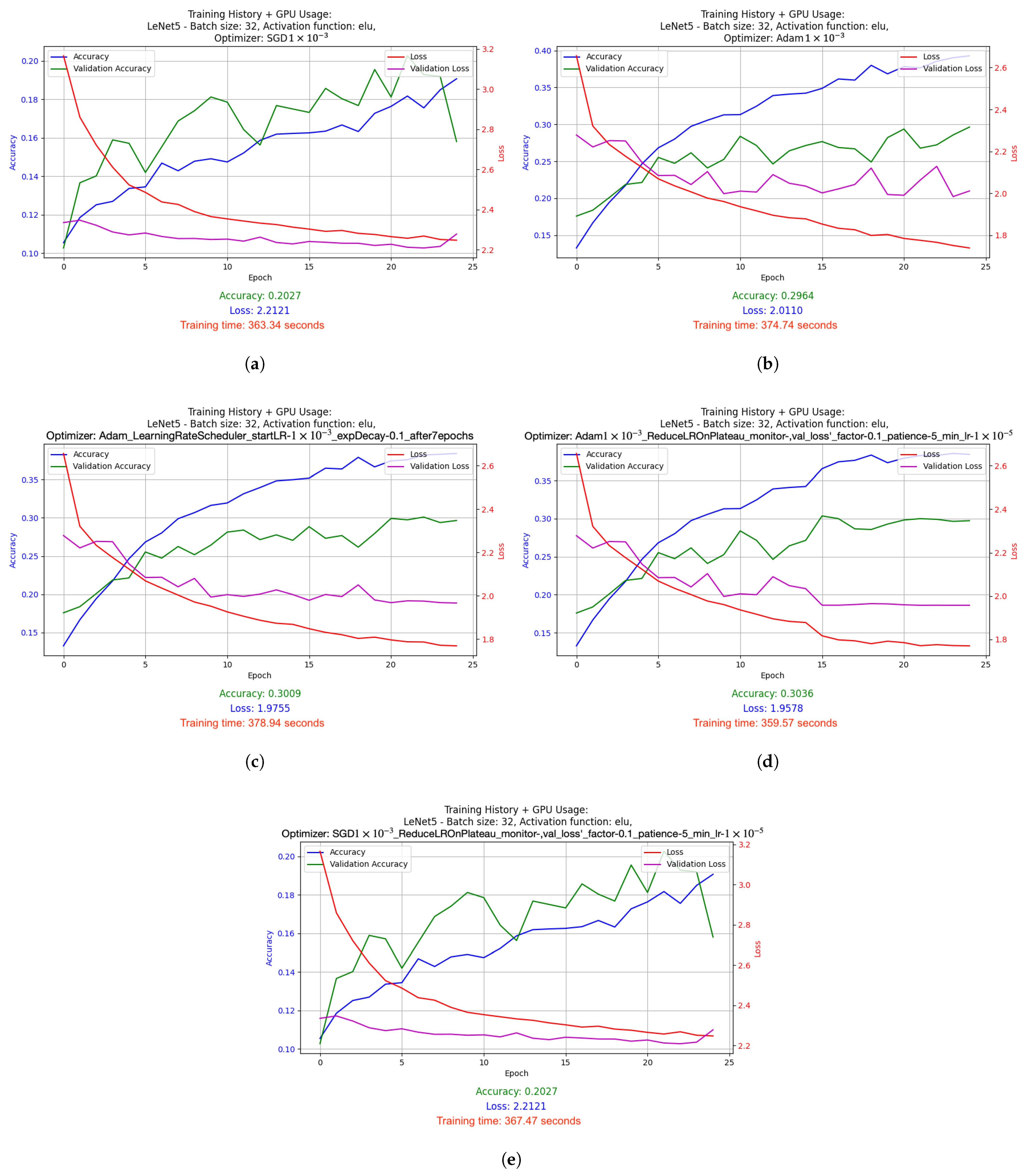
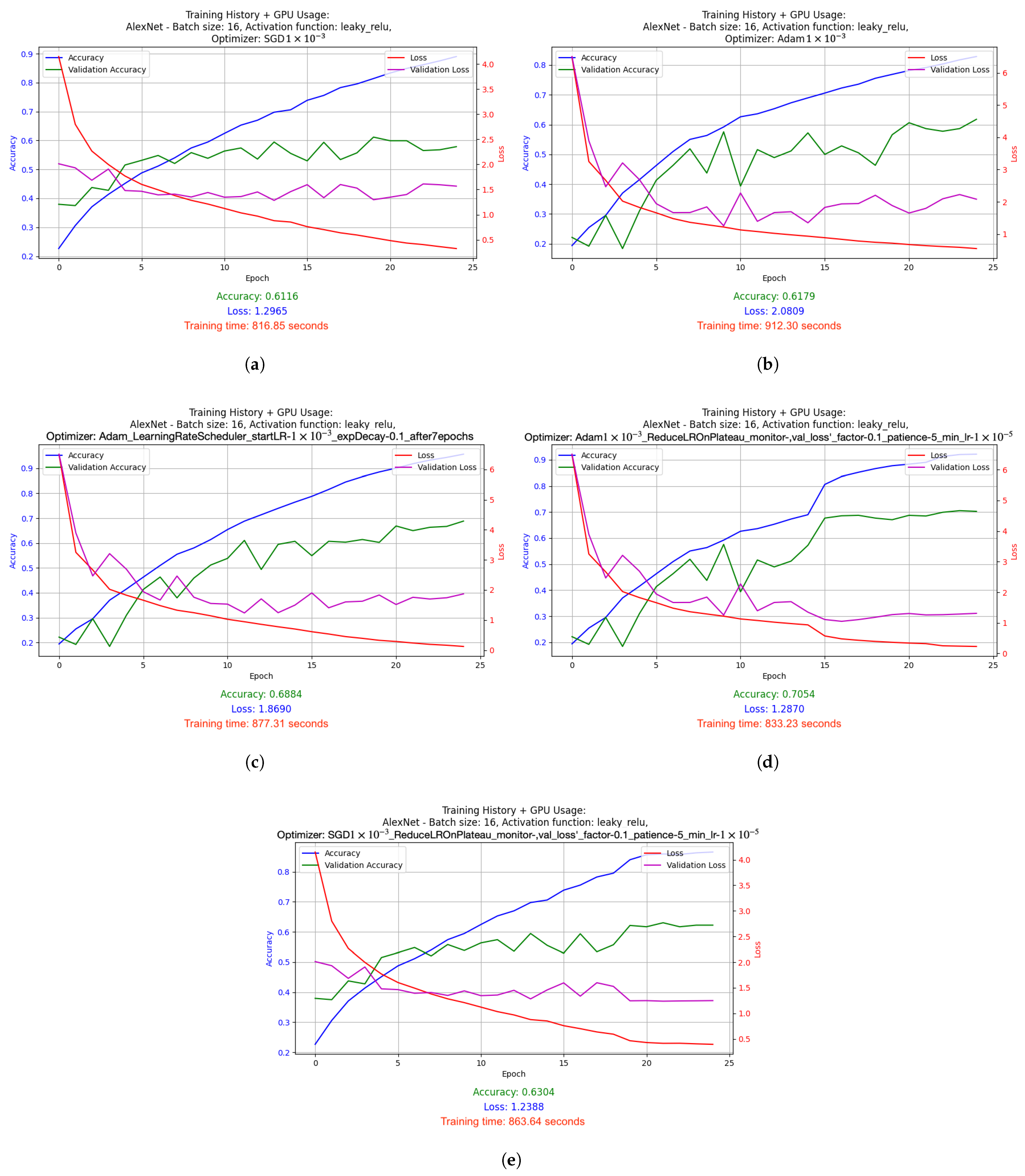
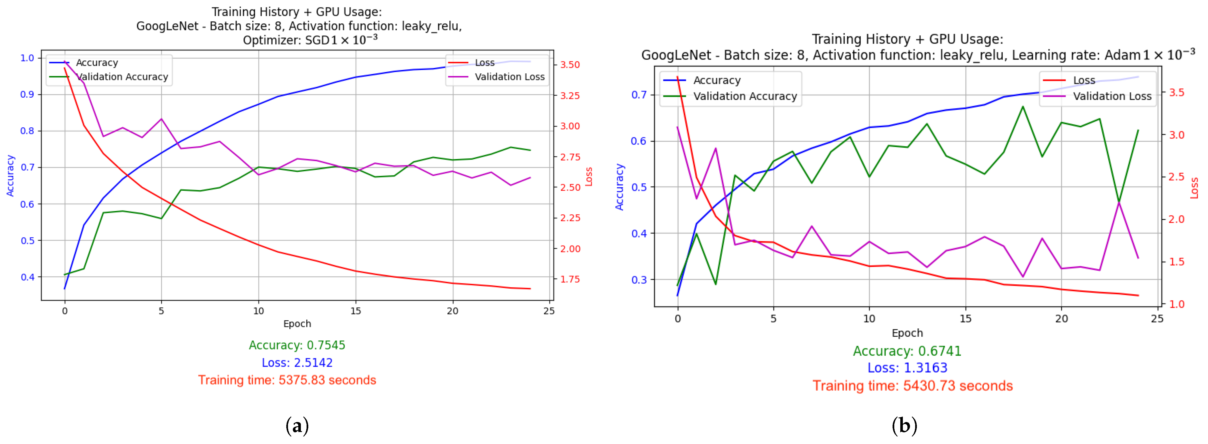
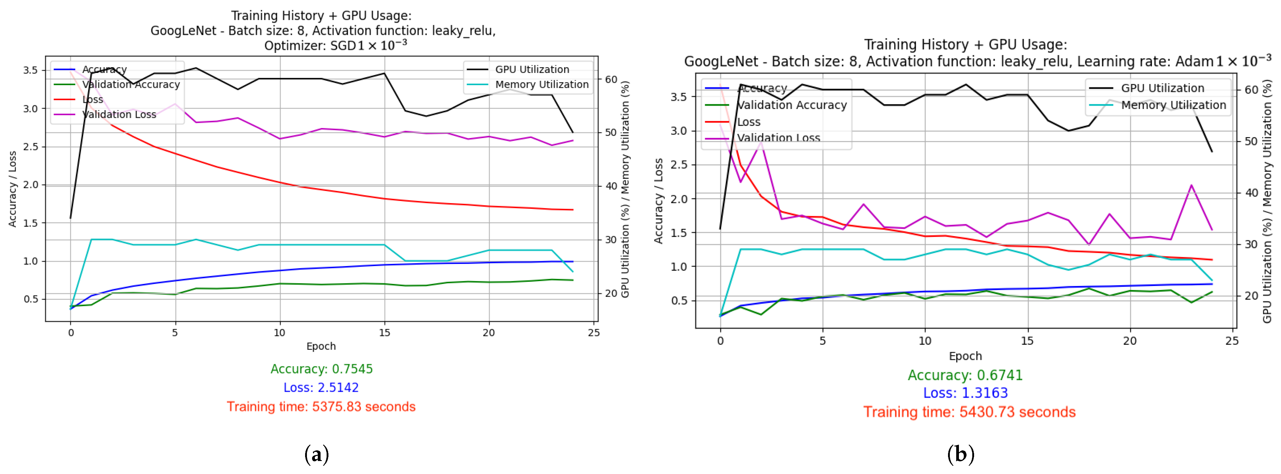
• SGD with LR = 1 × 10⁻³: Stochastic Gradient Descent (SGD) optimizer with a fixed, constant learning rate of 0.001. SGD is one of the simplest optimizers that updates the model weights based on the average gradient calculated for each batch (batch). The fixed learning rate causes the model to learns at a steady pace throughout the training.
• Adam with LR = 1 × 10⁻³: Adam optimizer, which is a more advanced version of the optimizer that combines the advantages of RMSprop and SGD with momentum. With a fixed learning rate of 0.001, Adam dynamically adjusts the weight update steps, which usually leads to faster and more stable convergence compared to classic SGD.
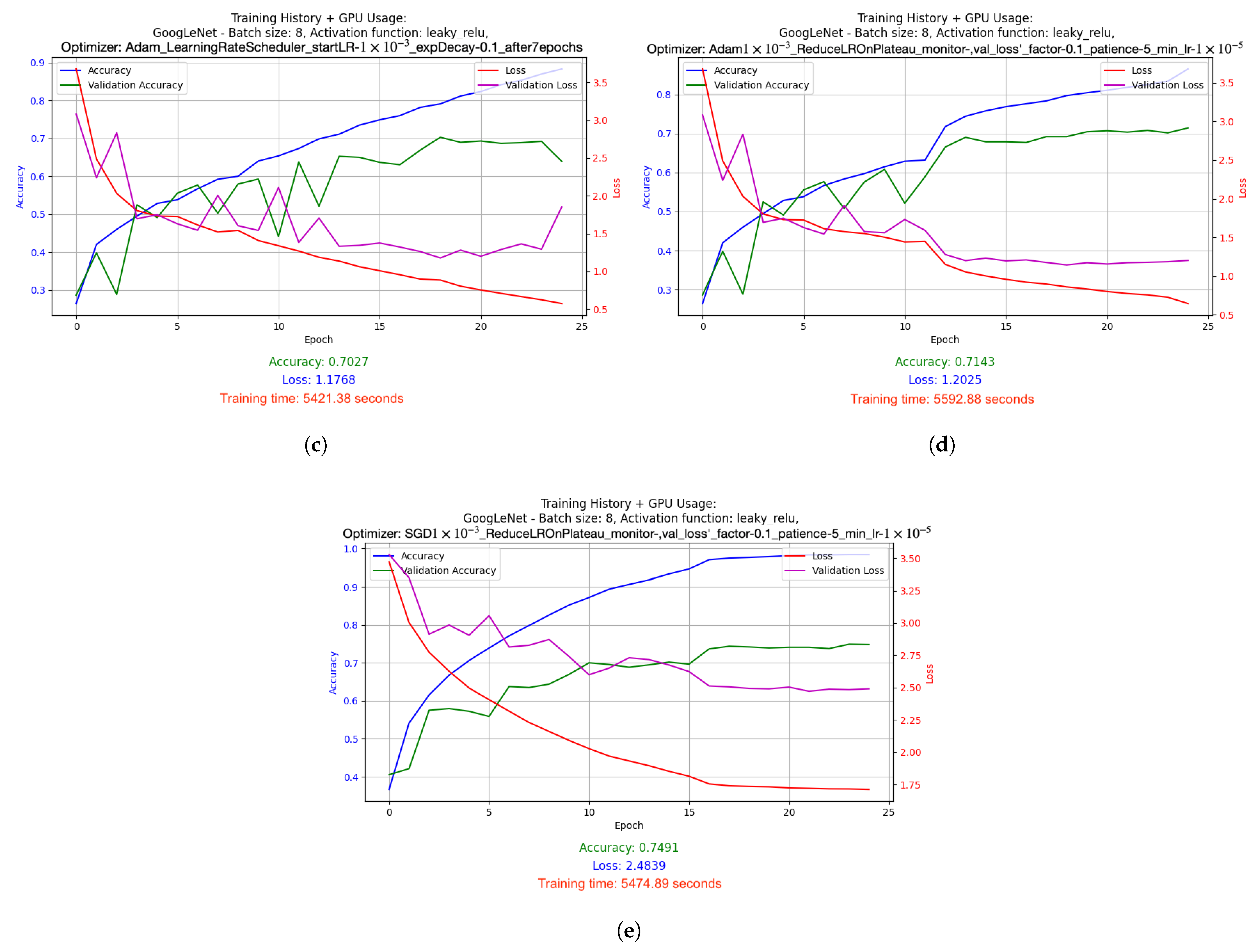
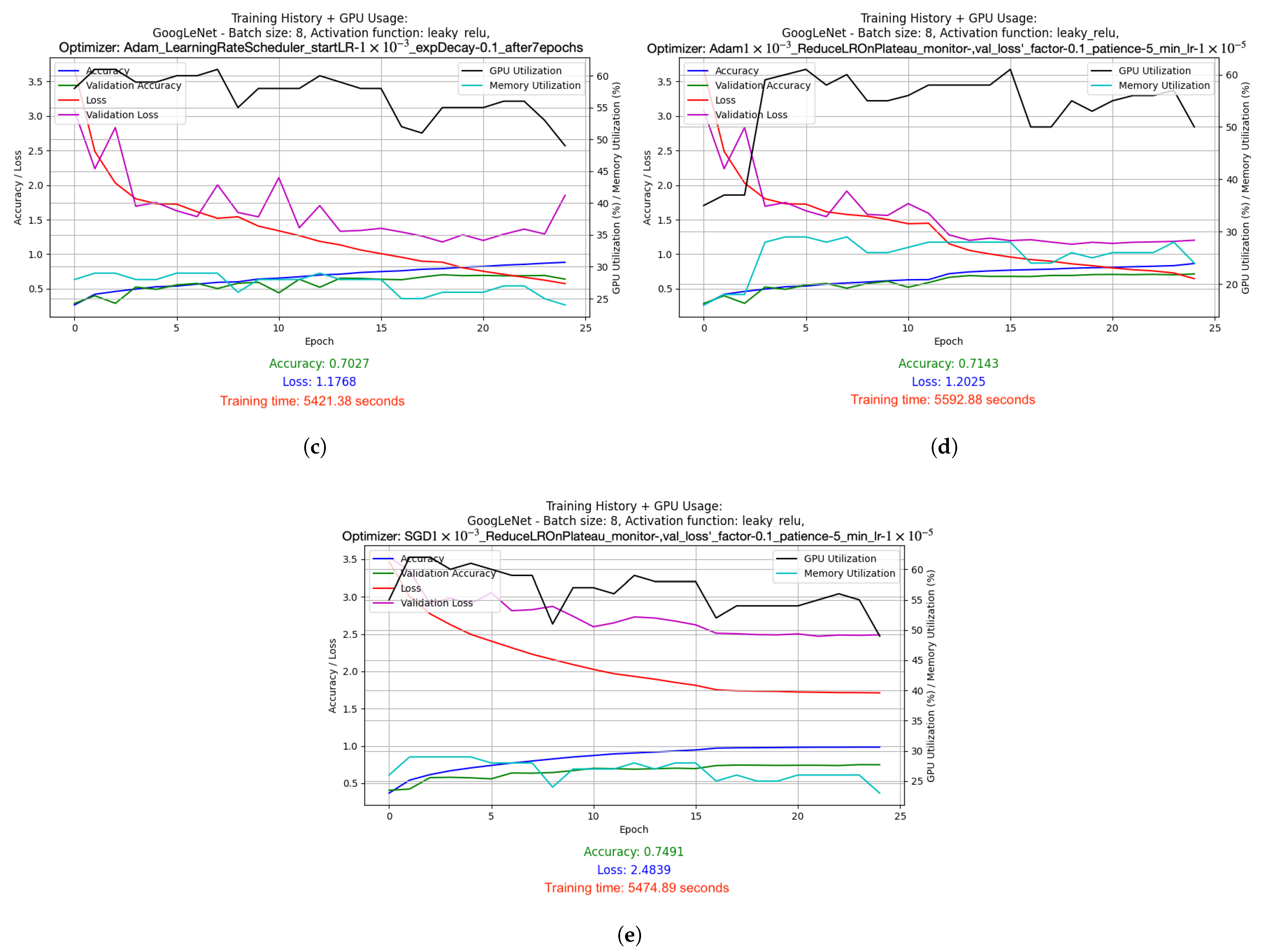
• Adam with dynamically adjusted LR using LearningRateScheduler: This setup used a starting learning rate of 0.001, which was dynamically reduced by a factor of 0.1 after 7 epochs of training. This mechanism allows for faster learning at the beginning, and then stabilizes the process as the model approaches the minimum of the cost function.
• Adam with LR reduced on Plateau: In this version, the learning factor was automatically reduced when it was noticed that the improvement in the value of the cost function stopped (i.e., when the value of val_loss stopped decreasing). The learning rate was reduced by a factor of 0.1 from its initial level of 0.001, and the minimum possible learning rate was set at 0.00001. This method allows the model to tune itself more accurately when it begins to reach the limits of its optimization capabilities.
• SGD with LR reduced on Plateau: Similar to Adam’s, here, the learning rate reduction mechanism was also used on Plateau, but in combination with the SGD optimizer. This allows better use of the simple mechanism for SGD to update the weights, especially in the later phases of training, where model accuracy requires finer adjustments.

LeNet-5

Figure 16 shows the effect of different learning strategies on the performance of the LeNet-5 model. Using the SGD optimizer with LR = 1 × 10⁻³ yielded the lowest accuracy of 20.27% and the highest loss of 2.21, suggesting that the model was unable to converge efficiently to optimal values. Introducing the Adam optimizer with the same learning rate improved the results, achieving an accuracy of 29.64% and a loss of 2.01. Applying the dynamic LR to Adam, where the initial LR was 1 × 10⁻³ with an exposure gradient, yielded even better results, with an accuracy of 30.09% and a loss of 1.98. The best results were obtained using the Adam optimizer with LR reduced on Plateau, achieving the highest accuracy of 30.36% and the lowest loss of 1.96. It was noted that the SDG optimizer with LR reduced on Plateau achieved very similar results to the regular SGD without additional modifications to the learning rate. The accuracy of both configurations was the same, at 20.27%, and the loss was also unchanged, remaining at 2.21. Moreover, the differences in training time were minimal, amounting to only about 4 s in favor of the strategy with learning rate reduction. This indicates that the optimizer did not change the learning rate setting throughout the learning period, as the model did not encounter a significant drop in loss improvement that would meet the conditions for triggering the learning rate reduction mechanism. As a result, the optimizer operated at a constant learning rate, suggesting that the reduction criteria were set too strictly for the learning rate change to be activated. Figure 17 presents GPU and memory consumption for different learning strategies. It is worth noting that GPU consumption was highest when using the Adam optimizer with LR = 1 × 10⁻³, at 9.32%. The lowest GPU consumption was observed using SGD, with a value of 8.72%, and SGD with Plateau reduction, with a value of 7.44%, but at the expense of poorer model accuracy. Dynamically adjusting LR in Adam resulted in relatively low GPU consumption (8.56%), while improving model accuracy and stability. Optimizing Adam with LR reduction on Plateau proved the most efficient in terms of GPU consumption, which was 8.72%, while maintaining high accuracy. During the training of the LeNet5 model, regardless of the optimization strategy used, GPU memory consumption settled around 3%. At the same time, RAM occupation remained at around 50%, and the average CPU usage was around 15%.

AlexNet

Figure 18 shows the results obtained when training the AlexNet model using different optimization strategies. The lowest accuracy of 61.16% and a loss of 1.30 were obtained using the SGD optimizer with LR = 1 × 10⁻³. Using the Adam optimizer with the same learning rate led to a slight increase in accuracy to 61.79%, but the loss increased to 2.08, indicating greater model instability. The introduction of dynamic LR in Adam led to a significant increase in accuracy to 68.84% with a loss of 1.87, suggesting a better fit of the model to the data. The Adam optimizer with LR reduced on Plateau achieved the highest accuracy of 70.54% and the lowest loss of 1.29, indicating an effective fit of the model parameters. When using the SGD with LR reduced on Plateau, the accuracy increased to 63.04% and the loss dropped to 1.24, a significant improvement over the regular SGD. Figure 19 shows GPU and memory consumption during training. GPU consumption peaked when using SGD with LR = 1 × 10⁻³, at 25.24%. Using the Adam optimizer brought GPU consumption down to 23.76%, but at the cost of a higher loss. Dynamically adjusting the LR in Adam reduced GPU consumption to 22.88%, while improving model performance. The most effective GPU utilization was recorded using the LR reduction strategy on Plateau for both the Adam and SGD optimizers, where utilization was 23.20% and 23.80%, respectively, with both strategies achieving significant improvements in accuracy and loss reduction. Regardless of the strategy used, RAM occupancy oscillated around 50-58%, and average CPU utilization remained around 15%.

GoogLeNet

Figure 20 shows the effect of different learning strategies on the performance of the GoogLeNet model. Using the SGD optimizer with LR = 1 × 10⁻³ provided the highest accuracy of 75.45% with a loss of 2.51, showing the good performance of this method. The Adam optimizer with the same learning rate yielded a slightly lower accuracy (67.41%) and a better loss of 1.31. The use of dynamic LR in Adam resulted in improved performance, achieving an accuracy of 70.27% and a loss of 1.17. The best results were achieved using the Adam optimizer with LR reduction on Plateau, where the accuracy was 71.43% and a loss of 1.20, while using the SGD optimizer with LR reduction on Plateau yielded very similar results to the regular SGD, achieving an accuracy of 74.91% and a loss of 2.48. Figure 21 presents GPU and memory consumption for different GoogLeNet model learning strategies. GPU usage ranged from 53.92% to 57.36%, with the highest usage recorded using the SGD optimizer with LR = 1 × 10⁻³. GPU memory usage remained at 25.72% to 27.8%. RAM occupation ranged from 47.9% to 52.21%, showing efficient management of memory resources. Average CPU utilization oscillated between 14.37% and 18.89%, indicating moderate CPU load during training. The best results in terms of resource efficiency and model performance were obtained using the Adam optimizer with LR reduction on Plateau.

Training results on full dataset for optimized models

Figure 22, Figure 23 and Figure 24 show the training history of three previously optimized neural network architectures: LeNet-5, AlexNet, and GoogLeNet. Each was trained on the full dataset for 50 epochs with hyperparameters tuned at an earlier stage of the study.

The results of the experiments are as follows:

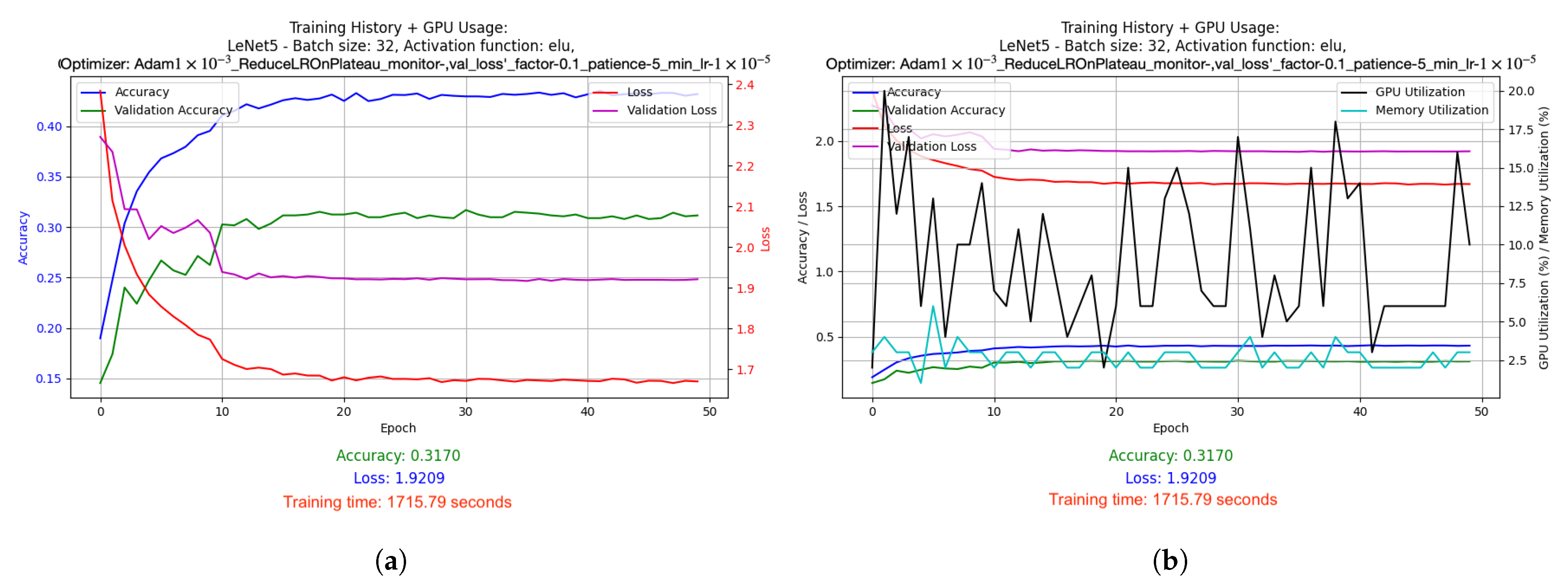
• LeNet-5 used batch size 32 and ELU activation function. It was optimized using the Adam algorithm (learning rate: 1 × 10⁻³) and the LR reduced on Plateau method. Results: accuracy 0.3170, loss 1.9209, average GPU usage 9.02%, average RAM usage 51.52%, training time 1715.79 s.
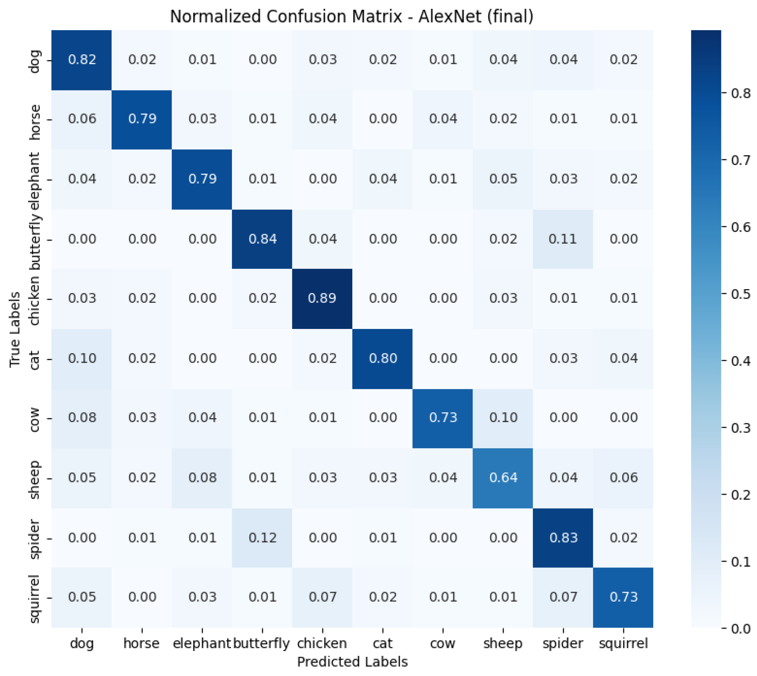
• AlexNet was trained with batch size 16 and Leaky ReLU activation function. Adam algorithm was used (learning rate: 1 × 10⁻³). Results: accuracy 0.7875, loss 1.0198, average GPU usage 23.48%, average RAM usage 50.55%, training time 4072.20 s.
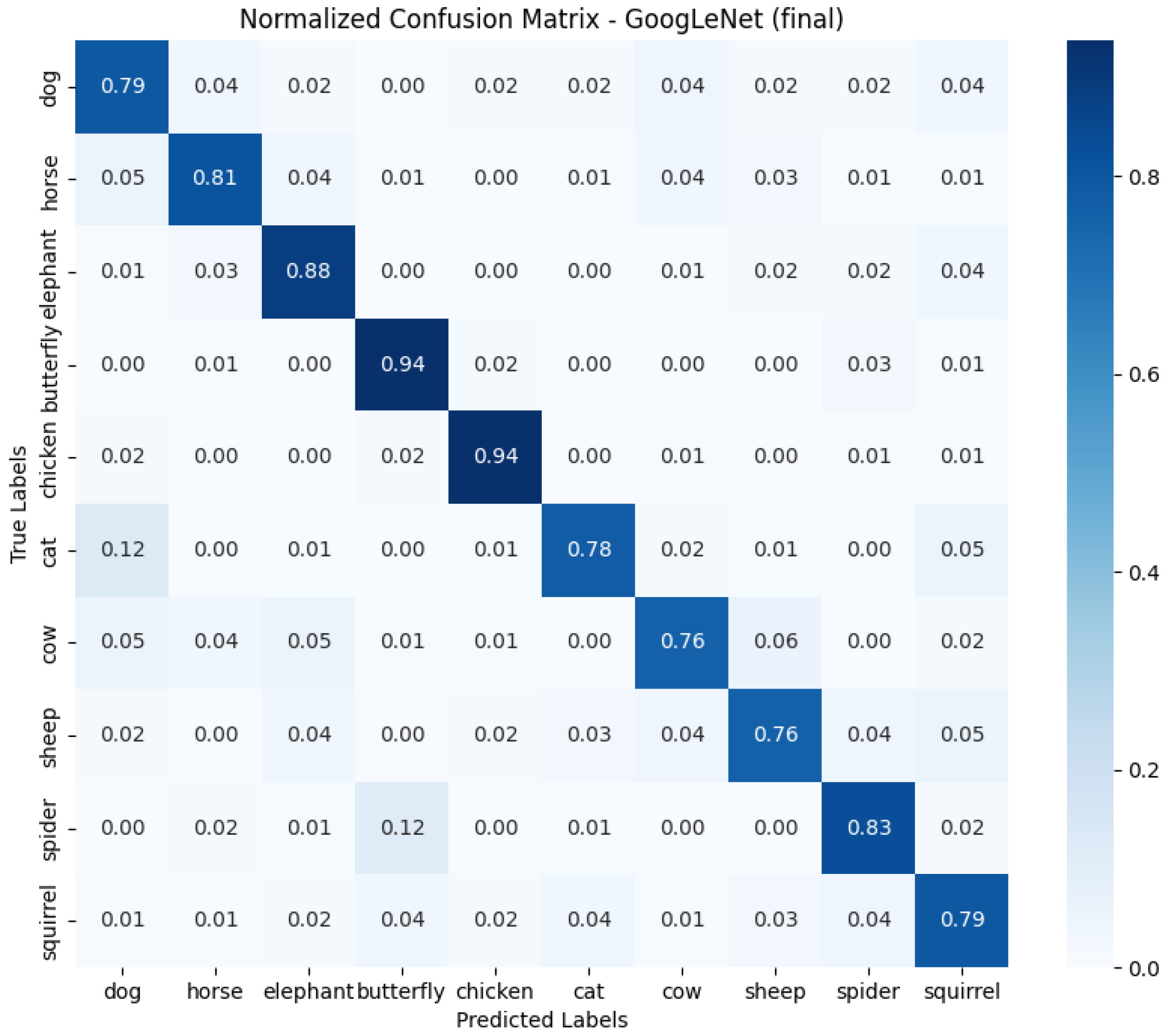
• GoogLeNet used batch size 8 and the Leaky ReLU activation function. Optimized with the Adam algorithm with a learning rate change schedule (learning rate: 1 × 10⁻³). Results: accuracy 0.8286, loss 1.0534, average GPU usage 58.62%, average RAM usage 52.12%, training time 25,251.97 s.

The GoogLeNet model, which achieved the highest accuracy, was selected for further testing.

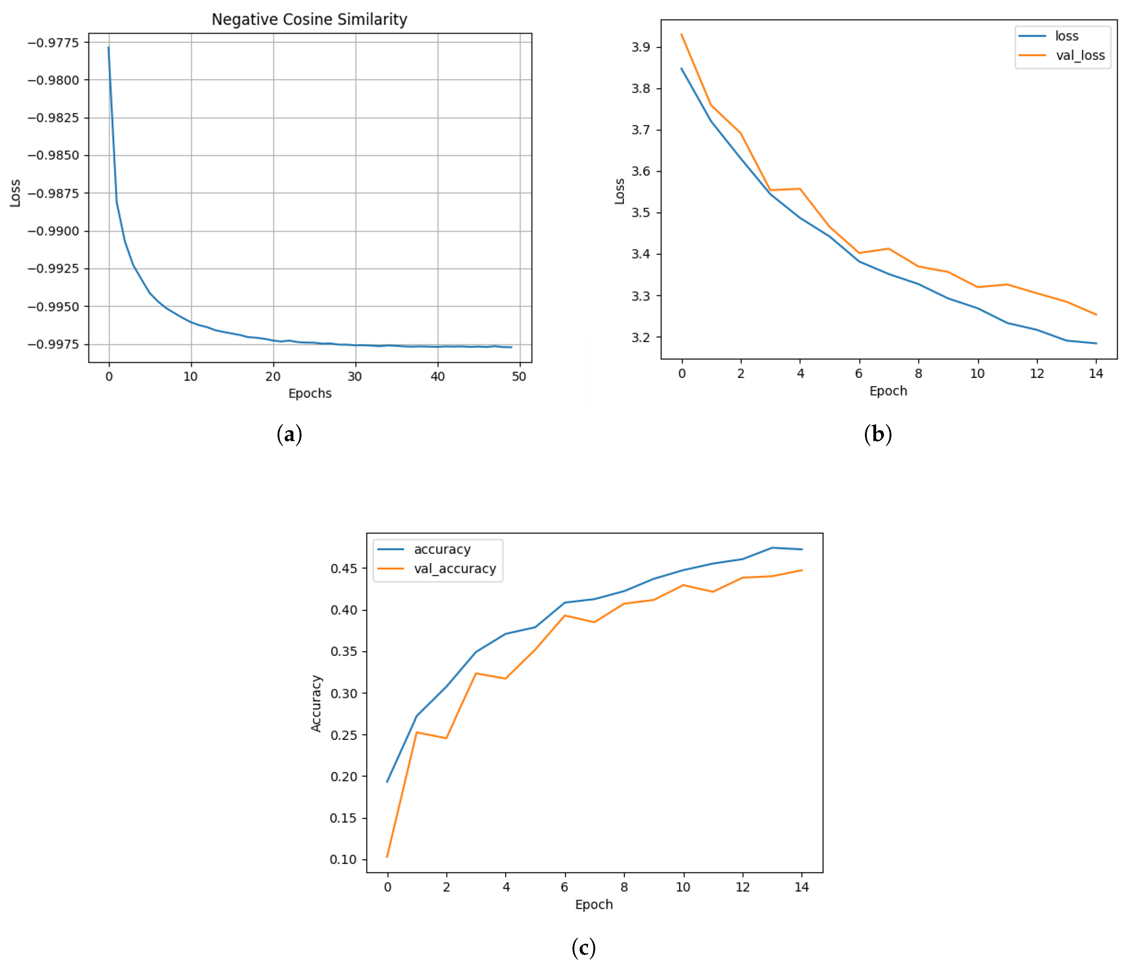
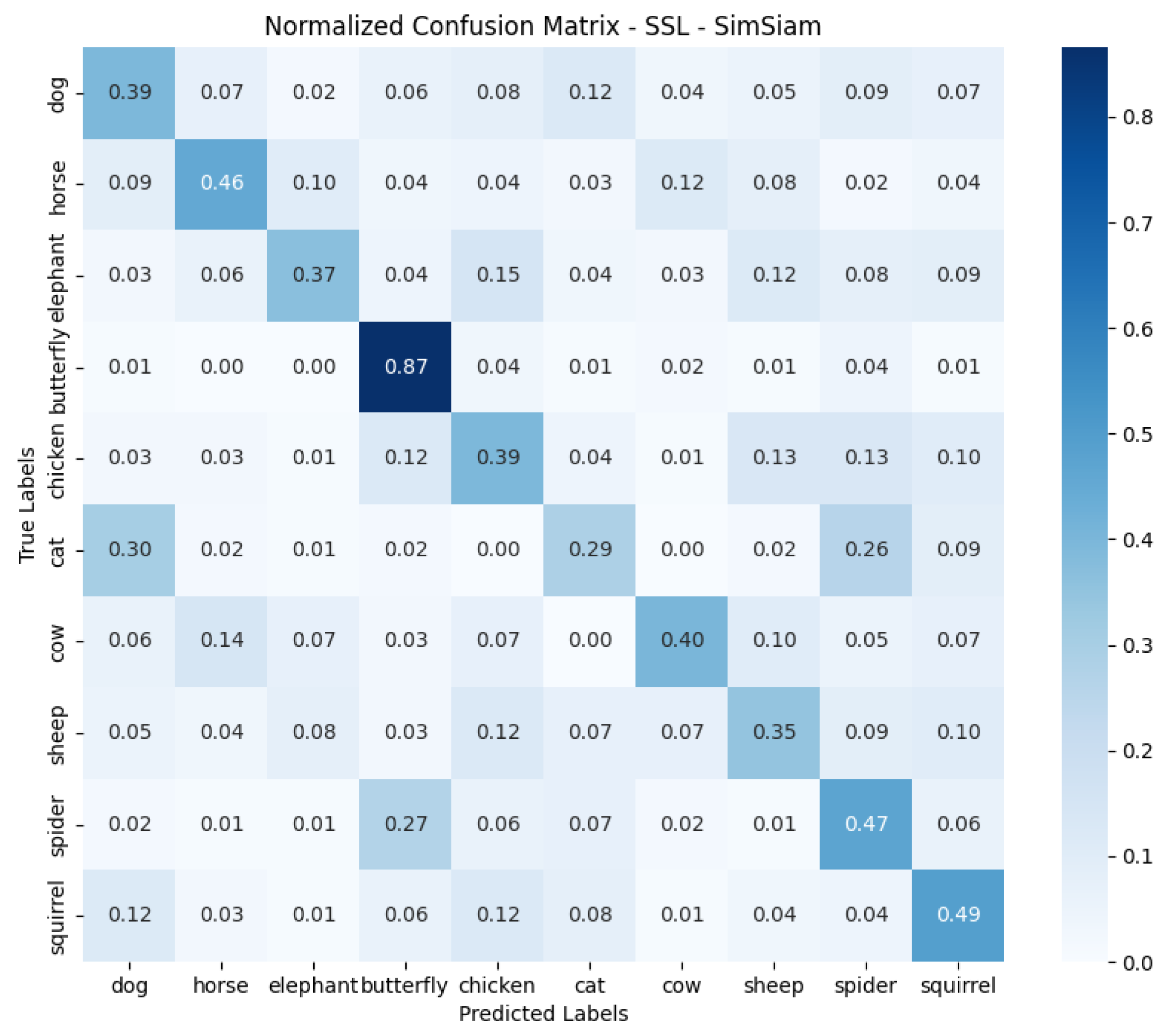
2.5.2. Experimental Results for Self-Supervised Learning Technique

Figure 25a illustrates the course of decreasing the loss function, based on the Negative Cosine Similarity measure, when training the model using the SimSiam technique. This measure assesses how similar two representations are in terms of angular similarity: the closer they are to each other, the smaller the value of this loss function. During training, this value gradually decreases and approaches −1, indicating an effective learning process for the model, which learns to increasingly group similar images in the representation space.

Figure 25b and Figure 25c show, respectively, the changes in loss metrics and accuracy during transfer learning with frozen weights on a model trained using SimSiam. The loss metric graph shows a gradual decrease in loss values, suggesting that the model is effectively adapting to the new task using previously learned representations. The accuracy graph, on the other hand, shows a systematic increase in accuracy, demonstrating that the model is getting better at classifying samples as training progresses.

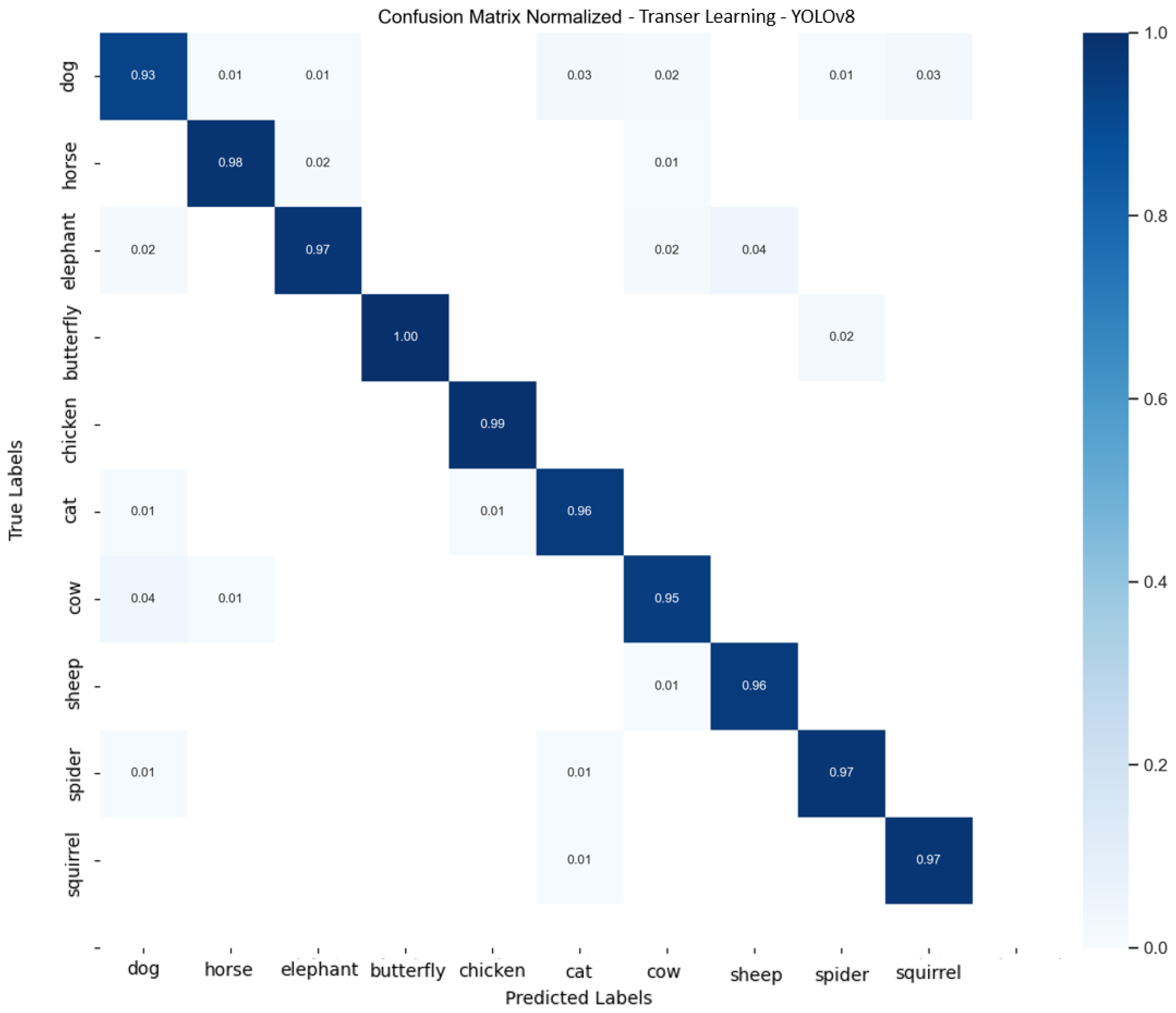
2.5.3. Experimental Results for the Transfer Learning Technique

The results in Figure 26 show a detailed learning process for the YOLOv8 model using the transfer learning technique.

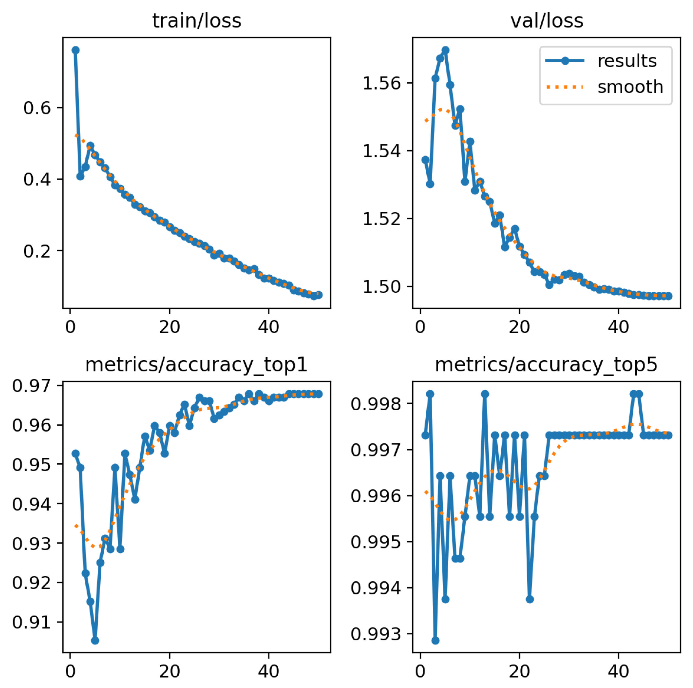
• Training loss graph (train/loss): This graph shows that training loss decreases steadily with each successive epoch, suggesting that the model adjusts effectively to the training data.
• Validation loss chart (val/loss): Despite initial fluctuations, validation losses are also decreasing, indicating an improvement in the model’s ability to generalize on new data.
• Accuracy of top-1 and top-5 classifications:

  –

  Top-1 Accuracy: A measure that indicates how often the correct label (class) is the highest rated by the model among all possible classes. In other words, it is the percentage of cases in which the model correctly predicts the most likely class.

  –

  Top-5 Accuracy: This metric measures how often the correct label is among the five highest rated classes by the model. Top-5 accuracy is used in tasks where there are many classes to choose from and it is possible that the model will identify several classes as potentially correct. This metric is more forgiving than top-1 because it allows for some margin of error.

These graphs show a gradual increase in classification accuracy, both for top-1 and top-5. Top-1 accuracy in particular shows significant improvement, confirming that the model is becoming more accurate in predicting first classes.

3. Discussion of Results

This section of the paper interprets the results obtained in research on optimizing neural network models. These results are discussed in the chapter on presentation of research results, where various approaches to training LeNet-5, AlexNet, and GoogLeNet models are presented. Comparison of different batch sizes: Analysis of the results showed that the size of the batch has a significant impact on the performance of the models. For the LeNet-5 model, a batch size of 32 proved to be the optimal choice, providing a balance between stability and training time. For the AlexNet model, on the other hand, a batch size of 16 proved optimal, offering good accuracy with efficient use of resources. GoogLeNet, as the most complex architecture, showed more variability in results depending on the batch size. The best results in terms of stability were obtained with a batch size of 8, but increasing the batch size to 32 resulted in improved accuracy and reduced training time. Effect of activation function on model performance: The activation functions proved crucial to the performance of the models, as confirmed by the experimental results. For the LeNet-5 model, the ReLU function, despite having the lowest accuracy, showed the lowest GPU consumption, suggesting its energy efficiency. Leaky ReLU proved to be the most efficient activation function for the GoogLeNet model, offering the best balance between accuracy and resource consumption. Effect of learning rate on model performance: Research on the learning rate has shown that dynamically adjusting this parameter during training brings significant benefits. Adam’s optimizer with dynamic learning rate allowed high accuracy while reducing the loss for all three models. The best results were obtained using a Plateau learning rate reduction strategy, confirming the high efficiency of this method in the context of optimizing neural network models. Results of final architecture training for optimal hyperparameters: The results of the final workouts for the LeNet-5, AlexNet, and GoogLeNet architectures, conducted on the full dataset using the best hyperparameter configurations, showed significant differences in the performance and efficiency of each architecture. LeNet-5, which is the least complex model, achieved the best training stability with a batch size of 32 and the Adam optimizer with Plateau learning rate reduction. For AlexNet, a batch size of 16 proved optimal, providing the best compromise between accuracy and training time. GoogLeNet, as the most complex of the architectures tested, performed best with larger batch sizes (32), which contributed to higher accuracy and shorter training times, albeit at the cost of greater variability in results.

Figure 27 shows the normalized confusion matrix for the LeNet-5 model, which represents the proportion of correct and incorrect classifications of each class, showing how well the model recognizes each class and which classes it most often confuses them with. The LeNet-5 model does a good job of classifying butterflies and spiders, as can be seen by the high values on the diagonal of the confusion matrix for these classes. However, the model often confuses other classes just with butterflies and spiders. This may indicate that the features that the model considers crucial for distinguishing between classes are more pronounced for butterflies and spiders, while for other classes, such as elephant, cat, sheep, and squirrel, these features are not sufficiently differentiating. The model obtains the worst results for the elephant, cat, sheep, and squirrel classes, which may be due to the similarity in visual features that the model considers important. For example, a squirrel is often mistaken for a spider, which may suggest that the model is misinterpreting certain details, such as texture or shape. Similarly, a dog barely matches its class better than that of a spider, indicating serious difficulties in distinguishing between the classes. Good scores for the butterfly may be due to its more distinct and unique visual features, such as the shape of its wings or their pattern, which are easily distinguished from those of other animals. Poor results for other classes, on the other hand, may be due to overly general features that the model has learned to recognize, leading to frequent classification errors. In this case, the model may not have learned to differentiate between these classes well enough, resulting in poor performance. The LeNet-5 model, which accepts images with a resolution of 32 × 32 pixels, may have encountered additional difficulties due to the pixelization of the original images, which likely had a higher resolution, such as around 200 × 200 pixels. Reducing the resolution to 32 × 32 leads to a loss of a lot of detail, which can significantly affect the model’s ability to accurately distinguish between classes. For classes such as elephant, cat, sheep, and squirrel, which may have more subtle visual differences, this loss of detail could cause problems with accurate classification. In addition, LeNet-5 operates on grayscale images, meaning that any information contained in color was also lost. This could have made it particularly difficult to distinguish between classes that have similar shapes but differ in color. In such cases, the model did not have access to the full visual information, which could lead to more frequent errors. These limitations may be a key reason why the model does well with classes such as butterfly and spider, which have clear outlines and distinctive shapes, but has problems with more complex or visually similar classes.

Figure 28 shows the normalized confusion matrix for the AlexNet model. The AlexNet model does very well in classifying such classes as dog, horse, elephant, butterfly, and chicken, as can be seen from the high values on the diagonal of the confusion matrix for these classes. In particular, the chicken (0.89) and the butterfly (0.84) stand out, which may suggest that these classes have features that are easily recognizable and clearly distinguishable from other classes. On the other hand, the most frequently confused classes are sheep, squirrel, and cow, which score the lowest. The sheep is often mistaken for a spider, which may indicate that the model has difficulty distinguishing texture or shape. AlexNet accepts images at a resolution of 227 × 227 pixels, which is much more detailed than LeNet-5. This allows the model to better distinguish details that can be crucial in classifying more complex classes. In addition, the model operates on RGB color scale images, which allows it to detect distinctive features based on color information as well. AlexNet’s results for classes such as butterfly and chicken are very good, which may be due to the unique visual features that these classes possess. However, the poorer results for other classes suggest that despite the higher resolution of the images, the model may still have trouble distinguishing between more similar classes.

Figure 29 shows the normalized confusion matrix for the GoogLe-Net model. The GoogLeNet model effectively classifies classes such as elephant, butterfly, and chicken, as evident in the high values on the diagonal of the matrix for these classes. In particular, the chicken (0.94) and butterfly (0.94) classes are recognized with high accuracy, suggesting that these categories have clear and easily recognizable features for the optimized GoogLeNet architecture. On the other hand, the model has difficulty correctly recognizing sheep, cat, and cow, as can be seen from the lower values on the diagonal and the relatively frequent misclassification of these classes. In the case of the cat class, the AlexNet architecture performs slightly better than GoogLeNet, which is surprising given that GoogLeNet is a more advanced and deeper network. This situation could be due to various factors. One possible reason is that AlexNet, despite its simpler architecture, can better match certain visual features of the cat, such as contours and shapes, which are less dependent on the very detailed analysis that GoogLeNet offers. In addition, deeper networks like GoogLeNet may be more prone to over-fitting more complex patterns, which can lead to poorer overall performance in distinguishing between classes with less complex features, such as cats. The GoogLeNet model operates on high-resolution images and the RGB color scale, which allows it to detect detailed visual features, including color information that can be crucial to correct classification. This is what makes the model so good at recognizing classes with distinct and unique features, such as a butterfly or a chicken. However, despite having access to full color information, the model can still have trouble distinguishing between classes with more subtle visual differences, such as cat and cow, which may explain the poorer results for these categories. In summary, three neural network architectures were analyzed: LeNet-5, AlexNet, and GoogLeNet, in terms of their effectiveness in classifying different classes of animals. LeNet-5, while doing well with some classes, such as butterfly and spider, has clear problems distinguishing between more complex categories, which may be due to its low resolution and work on grayscale images. AlexNet, on the other hand, offers better accuracy, especially for classes like cat and chicken, thanks to its work with RGB color scale images and higher resolution. GoogLeNet, despite being the deepest of the architectures analyzed, achieves very good results for most classes, but is slightly behind AlexNet for cat classification. A key role in achieving these satisfactory results was played by the hyperparameter optimization performed, which allowed each architecture to maximize its potential. Based on the analysis of graphs showing accuracy, loss, and resource consumption metrics (GPU, RAM, CPU), conclusions were drawn about the efficiency of the various configurations. These results identified the best performing configurations, which were then used in further experiments. Of the three architectures, GoogLeNet appears to be the best choice for further research, given its overall accuracy and ability to effectively classify a wide range of classes. Although AlexNet performs slightly better for the cat class, GoogLeNet’s overall performance is superior, making it a more versatile and reliable option for further research and applications in classification tasks. Results from the SimSiam approach: SimSiam, as a self-supervised learning technique, was applied to train the GoogLeNet model. The results show the effectiveness of this method in the context of representation learning. The value of the loss function, based on the inverse cosine similarity measure, systematically decreased, indicating an effective process of clustering similar images in the representation space. Although the method required a long training time (about 10 h for 50 epochs), the obtained accuracy was at a decent level of 0.4473 with a loss of 3.2532.

Figure 30 shows the normalized confusion matrix for the GoogLeNet model trained using the SSL SimSiam technique. The model shows the highest performance in classifying squirrel, spider, and butterfly, as can be seen from the relatively high values on the diagonal of the matrix for these categories, especially for butterfly (0.87). Nevertheless, the model clearly has problems distinguishing between classes such as elephant, cat, and sheep, where the values on the diagonal are much lower. Surprisingly, the cat class is recognized by the model with very low accuracy (0.29) and misclassified with higher probability as a dog, which may suggest that the characteristics the model considers key to this category are not sufficiently differentiated. This may be because the model with the GoogLeNet architecture, learned using a self-supervised learning approach, may have difficulty distinguishing between classes with less pronounced visual differences. The model, while using a sophisticated self-supervised learning approach, does not always handle more complex classes well, which may suggest the need for further tuning of hyperparameters or adapting the architecture to the specific requirements of the task. Comparing the GoogLeNet model to the SSL SimSiam model, which is also based on the GoogLeNet architecture, it can be seen that GoogLeNet in the standard supervised approach achieves better classification results. However, it is worth noting that the GoogLeNet model trained with the SimSiam self-supervised approach could give much better results if the training process lasted 100 to 200 epochs. Unfortunately, this approach is very time-consuming—already, 50 epochs of training took about 10 h. In addition, in order to maintain fairness and reliability of the results, the models were trained for the same number of epochs to fairly compare their performance. However, if the training time had been extended for the SSL approach using the SimSiam method, there is a high probability that it would have achieved even better performance, approaching and perhaps even surpassing the standard GoogLeNet results. The advantage of the self-supervised approach is that it does not require tagged data, which is a huge advantage, especially in the context of limited resources. Given that the model trained with the SSL approach achieved such good results even though we did not have labeled data, this is a very promising achievement that shows the potential of this approach in situations where access to labeled data is limited.

Results from the transfer learning approach

Transfer learning, using the YOLOv8 model, was applied to evaluate the effectiveness of adapting knowledge from pre-trained models to new tasks. Experimental results indicate that the method is effective, especially in the context of small datasets. Graphs showing changes in loss and accuracy metrics during training with frozen weights show a systematic decrease in loss values and an increase in accuracy, suggesting the effectiveness of this technique. The approach, despite initial fluctuations in validation loss, showed improvements in the model’s ability to generalize on new data, making transfer learning with YOLOv8 a particularly promising technique in the context of tasks requiring high-precision classification.

Figure 31 shows the normalized confusion matrix for the retrained YOLOv8 model by transfer learning. The matrix indicates high classification accuracy for most classes, which is particularly noticeable for categories such as butterfly, chicken, and horse, where the accuracy is 100%, 99%, and 98%, respectively. Despite minor matching errors for some classes, the transfer learning model with YOLOv8 generally achieves very high accuracy, which is particularly noteworthy given its ability to transfer previously learned representations to new classification tasks. This approach has a significant advantage in terms of speed of training and effective use of existing models. Training a model using the transfer learning method for a period of 50 epochs took less than one hour, making this approach the fastest among those tested. Summarizing and comparing the results of this model with the best results from previous approaches—optimized GoogLeNet from the classical supervised learning approach and GoogLeNet trained with the SSL SimSiam method—it can be seen that each model has its own unique advantages. GoogLeNet in the classical supervised approach stands out for its overall high accuracy and stability in classification, while GoogLe-Net trained with SSL SimSiam shows promising results, despite a smaller number of tagged data, with room for improvement with longer training. The transfer learning model with YOLOv8 is very efficient and effective, especially when limited computational and time resources are available, thanks to its ability to use existing representations. In terms of overall accuracy and performance, the transfer learning model with YOLOv8 achieved the best results in terms of matching, making it the most advanced and accurate model in this analysis. With its ability to transfer previously learned representations, YOLOv8 excelled in classification, achieving very high precision, especially in cases where accuracy and speed of classification are crucial. However, it should also be noted that GoogLeNet’s constructed and optimized model from the classical supervised approach has also demonstrated very good accuracy and stability in classification, making it a solid choice for applications where adequate computational and time resources are available to perform full training with labeled data.

4. Summary

The research conducted was aimed at optimizing neural network models and evaluating the effectiveness of various machine learning techniques in object detection tasks in images. The paper discusses in detail the results of experiments on the selection of hyperparameters, the comparison of different neural network architectures, and the comparison of the optimized architecture with the highest accuracy with other techniques such as self-supervised learning and transfer learning. Three main approaches were analyzed: supervised learning, self-supervised learning, and transfer learning, with different results in terms of object detection efficiency. The YOLOv8 model achieved the highest efficiency in the transfer learning approach, as confirmed by the results on classification accuracy and optimal use of computational resources. The results suggest that transfer learning, especially using pre-trained models, is a promising technique for tasks requiring fast training and high classification accuracy, especially in the context of small datasets. In the case of supervised learning, studies have shown that the technique, despite its effectiveness, is strongly dependent on the quality and quantity of labeled data. The GoogLeNet model used in this approach has achieved high accuracy in classifying objects in images, demonstrating its stability and effectiveness with large labeled datasets. However, the time-consuming nature of the data-labeling process is a significant limitation of this method. On the other hand, self-supervised learning (SSL), implemented using the SimSiam method, allowed a significant reduction in the dependence on labeled data, generating hidden labels from unstructured data. Despite the smaller number of labeled data, the method showed promising results, with the potential to further improve accuracy with increased training time. Compared to classic SL, the model trained with SSL achieved lower but still competitive accuracy, indicating the method’s great potential in the context of limited labeled data resources. The method achieved higher accuracy than the LeNet-5 model after 50 epochs on the full dataset, suggesting that the size of the images and the fact that LeNet-5 used black and white images have a more significant impact on the model’s performance than the data labeling itself in these particular approaches. This indicates the importance of appropriate training data selection and complexity in terms of achieving better object detection results. Several significant difficulties were encountered during the project:

• One of the biggest challenges was the limitation of computing resources. For very deep and complex architectures, such as GoogLeNet and GoogLe-Net in combination with SimSiam, memory started to run out at larger batch sizes, limiting the ability to test more resource-intensive hyperparameter values.
• Training more complex models, such as GoogLeNet and GoogLeNet+ SimSiam, was also very time-consuming. The long training time affected the performance of the project and translated into significant power consumption.
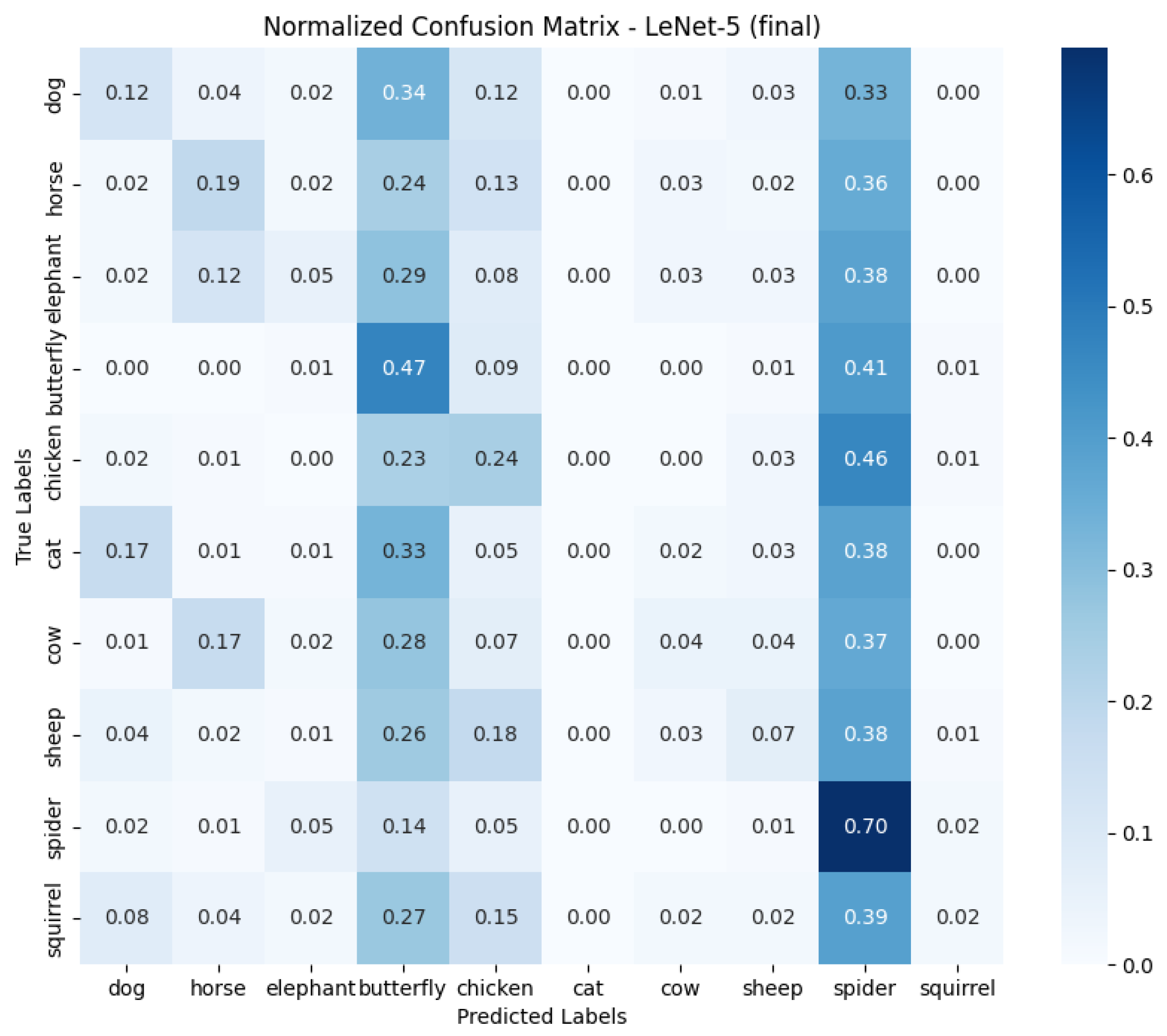
• Relatively low accuracy was obtained for the LeNet-5 model due to the architecture itself. LeNet-5 accepts small images that become pixelated during processing, leading to a significant loss of relevant information.
• Another difficulty was synchronizing versions of different tools, libraries, environments, and programming language. Compatibility issues often caused delays and required additional work to make sure all the system components worked harmoniously.
• Analyzing the results and selecting the best solution was also a challenge. Looking at the confusion matrix, different approaches did better with different classes of objects, making it difficult to clearly identify the best model. Final decisions were made based on the overall results, which may not have taken into account detailed differences in classification.
• Reliably assessing which configuration of hyperparameters was better when optimizing architectures in a supervised learning approach was also a difficulty. To cope with this problem, a proprietary training and model quality evaluation formula was created, which allowed a more precise analysis of the results. The project has opened the door to further development in several directions:
• Improving the LeNet-5 architecture: You might consider using a model that first determines the position of an object in an image and then cropping the image at that location. Reducing the image size to 32 × 32 pixels would then not cause so much pixelization, which could lead to better results while maintaining high speed.
• Optimizing the SimSiam model: The SimSiam model could be optimized for hyperparameters such as learning rate, and training time could be increased by increasing the number of epochs, which could contribute to better results.
• Confusion matrix analysis: A more thorough confusion matrix analysis could lead to improvements in the dataset for augmentation. The abundance of each data class could be equalized, especially where accuracy was weaker, which could improve the overall effectiveness of the models.
• Transfer learning: an interesting direction for further research would be to test transfer learning from the GoogLeNet model, obtained using the supervised learning method, on other data containing entirely new object classes. Comparing the results of such transfer learning with those obtained from the YOLOv8 model could provide valuable new insights into the effectiveness of these approaches in different contexts.

References

1. Budak, Ü.; Şengür, A.; Halici, U. Deep convolutional neural networks for airport detection in remote sensing images. In Proceedings of the 26th Signal Processing and Communications Applications Conference (SIU), Izmir, Turkey, 2–5 May 2018; pp. 1–4. [Google Scholar] [CrossRef]
2. Aitkenhead, M.; McDonald, A. A neural network face recognition system. Eng. Appl. Artif. Intell. 2003, 16, 167–176. [Google Scholar] [CrossRef]
3. Maitra, D.S.; Bhattacharya, U.; Parui, S.K. CNN based common approach to handwritten character recognition of multiple scripts. In Proceedings of the 2015 13th International Conference on Document Analysis and Recognition (ICDAR), Tunis, Tunisia, 23–26 August 2015; pp. 1021–1025. [Google Scholar] [CrossRef]
4. Chahuán-Jiménez, K. Neural Network-Based Predictive Models for Stock Market Index Forecasting. J. Risk Financ. Manag. 2024, 17, 242. [Google Scholar] [CrossRef]
5. Abhishek, K.; Singh, M.; Ghosh, S.; Anand, A. Weather Forecasting Model using Artificial Neural Network. Procedia Technol. 2012, 4, 311–318. [Google Scholar] [CrossRef]
6. Hemanth, D.J.; Estrela, V.V. Deep Learning for Image Processing Applications; IOS Press: Amsterdam, The Netherlands, 2017. [Google Scholar]
7. Sumathi, S.; Janani, M. Neural Networks for Natural Language Processing; IGI Global: Hershey, PA, USA, 2020. [Google Scholar] [CrossRef]
8. Sabharwal, N.; Agrawal, A. Neural Networks for Natural Language Processing. In Hands-On Question Answering Systems with BERT: Applications in Neural Networks and Natural Language Processing; Apress: Berkeley, CA, USA, 2021; pp. 15–39. [Google Scholar] [CrossRef]
9. Deng, J.; Dong, W.; Socher, R.; Li, L.J.; Li, K.; Fei-Fei, L. ImageNet: A large-scale hierarchical image database. In Proceedings of the 2009 IEEE Conference on Computer Vision and Pattern Recognition, Miami, FL, USA, 20–25 June2009; pp. 248–255. [Google Scholar] [CrossRef]
10. Russakovsky, O.; Deng, J.; Su, H.; Krause, J.; Satheesh, S.; Ma, S.; Huang, Z.; Karpathy, A.; Khosla, A.; Bernstein, M.; et al. ImageNet Large Scale Visual Recognition Challenge. Int. J. Comput. Vis. 2015, 115, 211–252. [Google Scholar] [CrossRef]
11. Bappy, J.H.; Roy-Chowdhury, A.K. CNN based region proposals for efficient object detection. In Proceedings of the 2016 IEEE International Conference on Image Processing (ICIP), Phoenix, AZ, USA, 25–28 September 2016; pp. 3658–3662. [Google Scholar] [CrossRef]
12. Zhao, Z.; Alzubaidi, L.; Zhang, J.; Duan, Y.; Gu, Y. A comparison review of transfer learning and self-supervised learning: Definitions, applications, advantages and limitations. Expert Syst. Appl. 2024, 242, 122807. [Google Scholar] [CrossRef]
13. Michalski, B.; Plechawska-Wójcik, M. Comparison of LeNet-5, AlexNet and GoogLeNet models in handwriting recognition. J. Comput. Sci. Inst. 2022, 23, 145–151. [Google Scholar] [CrossRef]
14. Iqbal, S.; Qureshi, A.N.; Ullah, A.; Li, J.; Mahmood, T. Improving the Robustness and Quality of Biomedical CNN Models through Adaptive Hyperparameter Tuning. Appl. Sci. 2022, 12, 11870. [Google Scholar] [CrossRef]
15. Nugraha, G.S.; Darmawan, M.I.; Dwiyansaputra, R. Comparison of CNN’s architecture GoogleNet, AlexNet, VGG-16, Lenet-5, Resnet-50 in Arabic handwriting pattern recognition. Kinet. Game Technol. Inf. Syst. Comput. Netw. Comput. Electron. Control 2023, 8. [Google Scholar] [CrossRef]
16. Zhu, Y.; Li, G.; Wang, R.; Tang, S.; Su, H.; Cao, K. Intelligent fault diagnosis of hydraulic piston pump combining improved LeNet-5 and PSO hyperparameter optimization. Appl. Acoust. 2021, 183, 108336. [Google Scholar] [CrossRef]
17. Imen, W.; Amna, M.; Fatma, B.; Ezahra, S.F.; Masmoudi, N. Fast HEVC intra-CU decision partition algorithm with modified LeNet-5 and AlexNet. SIgnal Image Video Process. 2022, 16, 1811–1819. [Google Scholar] [CrossRef]
18. Ramesh Babu, P.; Srikrishna, A.; Gera, V.R. Diagnosis of tomato leaf disease using OTSU multi-threshold image segmentation-based chimp optimization algorithm and LeNet-5 classifier. J. Plant Dis. Prot. 2024, 131, 2221–2236. [Google Scholar] [CrossRef]
19. Ha, K.W.; Park, S.; Chon, S.; Kim, J.K.; Jung, S. A SimSiam-based Generalized Model Training Technique for Classification of ECG from Heterogeneous Devices. In Proceedings of the 2023 IEEE International Conference on Big Data and Smart Computing (BigComp), Jeju, Republic of Korea, 13–16 February 2023; pp. 312–313. [Google Scholar] [CrossRef]
20. Aboutorab, H.; Hussain, O.K.; Saberi, M.; Hussain, F.K.; Chang, E. A survey on the suitability of risk identification techniques in the current networked environment. J. Netw. Comput. Appl. 2021, 178, 102984. [Google Scholar] [CrossRef]
21. YOLOv8 Description. Available online: https://yolov8.com/ (accessed on 30 August 2024).
22. Raiaan, M.A.K.; Sakib, S.; Fahad, N.M.; Mamun, A.A.; Rahman, M.A.; Shatabda, S.; Mukta, M.S.H. A systematic review of hyperparameter optimization techniques in Convolutional Neural Networks. Decis. Anal. J. 2024, 11, 100470. [Google Scholar] [CrossRef]
23. Wojciuk, M.; Swiderska-Chadaj, Z.; Siwek, K.; Gertych, A. Improving classification accuracy of fine-tuned CNN models: Impact of hyperparameter optimization. Heliyon 2024, 10, e26586. [Google Scholar] [CrossRef] [PubMed]
24. Aguerchi, K.; Jabrane, Y.; Habba, M.; El Hassani, A.H. A CNN Hyperparameters Optimization Based on Particle Swarm Optimization for Mammography Breast Cancer Classification. J. Imaging 2024, 10, 30. [Google Scholar] [CrossRef] [PubMed]
25. Jian, L.; Pu, Z.; Zhu, L.; Yao, T.; Liang, X. SS R-CNN: Self-Supervised Learning Improving Mask R-CNN for Ship Detection in Remote Sensing Images. Remote Sens. 2022, 14, 4383. [Google Scholar] [CrossRef]
26. Hojjati, H.; Ho, T.K.K.; Armanfard, N. Self-supervised anomaly detection in computer vision and beyond: A survey and outlook. Neural Netw. 2024, 172, 106106. [Google Scholar] [CrossRef] [PubMed]
27. Yang, J.; Lin, F.; Xiang, Y.; Katranuschkov, P.; Scherer, R.J. Fast Crack Detection Using Convolutional Neural Network. In EG-ICE 2021 Workshop on Intelligent Computing in Engineering; Abualdenien, J., Borrmann, A., Ungureanu, L.C., Hartmann, T., Eds.; Universitätsverlag der TU Berlin: Berlin, Germany, 2021; pp. 540–549. [Google Scholar] [CrossRef]
28. Lecun, Y.; Bottou, L.; Bengio, Y.; Haffner, P. Gradient-based learning applied to document recognition. Proc. IEEE 1998, 86, 2278–2324. [Google Scholar] [CrossRef]
29. Poonkuntran, S.; Dhanraj, R.; Balusamy, B. Object Detection with Deep Learning Models: Principles and Applications; Taylor & Francis Limited: Abingdon, UK, 2022. [Google Scholar] [CrossRef]
30. Lee, Y.; Kim, J. PSI Analysis of Adversarial-Attacked DCNN Models. Appl. Sci. 2023, 13, 9722. [Google Scholar] [CrossRef]
31. Yu, X.; Wang, S.H.; Zhang, X.; Zhang, Y.D. Detection of COVID-19 by GoogLeNet-COD. In Intelligent Computing Theories and Application; Huang, D.S., Bevilacqua, V., Hussain, A., Eds.; Springer International Publishing: Berlin/Heidelberg, Germany, 2020; pp. 499–509. [Google Scholar] [CrossRef]
32. Szegedy, C.; Liu, W.; Jia, Y.; Sermanet, P.; Reed, S.; Anguelov, D.; Erhan, D.; Vanhoucke, V.; Rabinovich, A. Going deeper with convolutions. In Proceedings of the 2015 IEEE Conference on Computer Vision and Pattern Recognition (CVPR), Boston, MA, USA, 7–12 June 2015; pp. 1–9. [Google Scholar] [CrossRef]
33. Animals-10 Dataset Description. Available online: https://www.kaggle.com/datasets/alessiocorrado99/animals10 (accessed on 30 September 2024).
34. Brownlee, J. Better Deep Learning: Train Faster, Reduce Overfitting, and Make Better Predictions; Machine Learning Mastery: San Francisco, CA, USA, 2018. [Google Scholar]
Figure 1. LeNet-5 network architecture diagram [28].
Applsci 15 07931 g001
Figure 2. AlexNet network architecture diagram [30].
Applsci 15 07931 g002
Figure 3. GoogLeNet network architecture diagram [32].
Applsci 15 07931 g003
Figure 4. Comparison of the results of the LeNet-5 model training process at different batch sizes. (a) Results for batch size = 8. (b) Results for batch size = 16. (c) Results for batch size = 32.
Applsci 15 07931 g004
Figure 5. Comparison of the results of the LeNet-5 model training process at different batch sizes, including GPU and memory consumption. (a) Results for batch size = 8. (b) Results for batch size = 16. (c) Results for batch size = 32.
Applsci 15 07931 g005
Figure 6. Comparison of the results of the AlexNet model training process at different batch sizes. (a) Results for batch size = 8. (b) Results for batch size = 16. (c) Results for batch size = 32.
Applsci 15 07931 g006
Figure 7. Comparison of the results of the AlexNet model training process at different batch sizes, including GPU and memory consumption. (a) Results for batch size = 8. (b) Results for batch size = 16. (c) Results for batch size = 32.
Applsci 15 07931 g007
Figure 8. Comparison of GoogLeNet model training process results at different batch sizes. (a) Results for batch size = 8. (b) Results for batch size = 16. (c) Results for batch size = 32.
Applsci 15 07931 g008
Figure 9. Comparison of the results of the GoogLeNet model training process at different batch sizes, including GPU and memory consumption. (a) Results for batch size = 8. (b) Results for batch size = 16. (c) Results for batch size = 32.
Applsci 15 07931 g009
Figure 10. Comparison of the results of the LeNet-5 model training process with different activation functions. (a) Results for ReLU. (b) Results for Leaky ReLU. (c) Results for ELU.
Applsci 15 07931 g010
Figure 11. Comparison of GPU and memory consumption during training of LeNet-5 model with different activation functions. (a) GPU and memory consumption for ReLU. (b) GPU and memory consumption for Leaky ReLU. (c) GPU and memory consumption for ELU.
Applsci 15 07931 g011
Figure 12. Comparison of the results of the AlexNet model training process with different activation functions. (a) Results for ReLU. (b) Results for Leaky ReLU. (c) Results for ELU.
Applsci 15 07931 g012
Figure 13. Comparison of GPU and memory consumption during training of AlexNet model with different activation functions. (a) GPU and memory consumption for ReLU. (b) GPU and memory consumption for Leaky ReLU. (c) GPU and memory consumption for ELU.
Applsci 15 07931 g013
Figure 14. Comparison of the results of the GoogLeNet model training process with different activation functions. (a) Results for ReLU. (b) Results for Leaky ReLU. (c) Results for ELU.
Applsci 15 07931 g014
Figure 15. Comparison of GPU and memory consumption during training of GoogLeNet model with different activation functions. (a) GPU and memory consumption for ReLU. (b) GPU and memory consumption for Leaky ReLU. (c) GPU and memory consumption for ELU.
Applsci 15 07931 g015
Figure 16. Comparison of the results of the LeNet-5 model training process at different learning rates. (a) Results for SGD with LR = 1 × 10⁻³. (b) Results for Adam with LR = 1 × 10⁻³. (c) Results for Adam with dynamically adjusted LR. (d) Results for Adam with LR reduced on Plateau. (e) Results for SGD with LR reduced on Plateau.
Applsci 15 07931 g016
Figure 17. Comparison of GPU and memory consumption when training the LeNet-5 model at different learning rates. (a) GPU and memory consumption for SGD with LR = 1 × 10⁻³. (b) GPU and memory consumption for Adam with LR = 1 × 10⁻³. (c) GPU and memory consumption for Adam with dynamically adjustable LR. (d) GPU and memory consumption for Adam with LR reduced on Plateau. (e) GPU and memory consumption for SGD with LR reduced on Plateau.
Applsci 15 07931 g017
Figure 18. Comparison of the results of the AlexNet model training process at different learning rates. (a) Results for SGD with LR = 1 × 10⁻³. (b) Results for Adam with LR = 1 × 10⁻³. (c) Results for Adam with dynamically adjusted LR. (d) Results for Adam with LR reduced on Plateau. (e) Results for SGD with LR reduced on Plateau.
Applsci 15 07931 g018
Figure 19. Comparison of GPU and memory consumption when training the AlexNet model at different learning rates. (a) GPU and memory consumption for SGD with LR = 1 × 10⁻³. (b) GPU and memory consumption for Adam with LR = 1 × 10⁻³. (c) GPU and memory consumption for Adam with dynamically adjustable LR. (d) GPU and memory consumption for Adam with LR reduced on Plateau. (e) GPU and memory consumption for SGD with LR reduced on Plateau.
Applsci 15 07931 g019
Figure 20. Comparison of the results of the GoogLeNet model training process at different learning rates. (a) Results for SGD with LR = 1 × 10⁻³. (b) Results for Adam with LR = 1 × 10⁻³. (c) Results for Adam with dynamically adjusted LR. (d) Results for Adam with LR reduced on Plateau. (e) Results for SGD with LR reduced on Plateau.
Applsci 15 07931 g020aApplsci 15 07931 g020b
Figure 21. Comparison of GPU and memory consumption when training the GoogLeNet model at different learning rates. (a) GPU and memory consumption for SGD with LR = 1 × 10⁻³. (b) GPU and memory consumption for Adam with LR = 1 × 10⁻³. (c) GPU and memory consumption for Adam with dynamically adjustable LR. (d) GPU and memory consumption for Adam with LR reduced on Plateau. (e) GPU and memory consumption for SGD with LR reduced on Plateau.
Applsci 15 07931 g021aApplsci 15 07931 g021b
Figure 22. LeNet-5 model results on the full dataset. (a) Training history of the optimized LeNet-5 model. (b) GPU and memory consumption during training of the optimized LeNet-5 model.
Applsci 15 07931 g022
Figure 23. AlexNet model results on the full dataset. (a) Training history of the optimized AlexNet model. (b) GPU and memory consumption during training of the optimized AlexNet model.
Applsci 15 07931 g023
Figure 24. GoogLeNet model results on the full dataset. (a) Training history of the optimized GoogLeNet model. (b) GPU and memory consumption during training of the optimized GoogLeNet model.
Applsci 15 07931 g024
Figure 25. Results for the model obtained using the SimSiam technique. (a) Loss—Negative Cosine Similarity for model SimSiam. (b) Learning process—loss metric (transfer learning with frozen weights). (c) Learning process—accuracy metrics (transfer learning with frozen weights).
Applsci 15 07931 g025
Figure 26. Graphs showing the training process of the YOLOv8 model using transfer learning. The top graphs show the changes in losses (train/loss, val/loss), and the bottom graphs show the accuracy of top-1 and top-5 classifications (metrics/accuracy_top1, metrics/accuracy_top5).
Applsci 15 07931 g026
Figure 27. Normalized confusion matrix for the LeNet-5 model.
Applsci 15 07931 g027
Figure 28. Normalized confusion matrix for the AlexNet model.
Applsci 15 07931 g028
Figure 29. Normalized confusion matrix for the GoogLeNet model.
Applsci 15 07931 g029
Figure 30. Normalized confusion matrix for the GoogLeNet model trained using the SSL SimSiam technique.
Applsci 15 07931 g030
Figure 31. Normalized confusion matrix for the retrained YOLOv8 model by transfer learning method.
Applsci 15 07931 g031
Disclaimer/Publisher’s Note: The statements, opinions and data contained in all publications are solely those of the individual author(s) and contributor(s) and not of MDPI and/or the editor(s). MDPI and/or the editor(s) disclaim responsibility for any injury to people or property resulting from any ideas, methods, instructions or products referred to in the content.