Uncertainty-Aware Predictive Process Monitoring in Healthcare: Explainable Insights into Probability Calibration for Conformal Prediction

Abstract

In high-stakes decision-making environments, predictive models must deliver not only high accuracy but also reliable uncertainty estimations and transparent explanations. This study explores the integration of probability calibration techniques with Conformal Prediction (CP) within a predictive process monitoring (PPM) framework tailored to healthcare analytics. CP is renowned for its distribution-free prediction regions and formal coverage guarantees under minimal assumptions; however, its practical utility critically depends on well-calibrated probability estimates. We compare a range of post-hoc calibration methods—including parametric approaches like Platt scaling and Beta calibration, as well as non-parametric techniques such as Isotonic Regression and Spline calibration—to assess their impact on aligning raw model outputs with observed outcomes. By incorporating these calibrated probabilities into the CP framework, our multilayer analysis evaluates improvements in prediction region validity, including tighter coverage gaps and reduced minority error contributions. Furthermore, we employ SHAP-based explainability to explain how calibration influences feature attribution for both high-confidence and ambiguous predictions. Experimental results on process-driven healthcare data indicate that the integration of calibration with CP not only enhances the statistical robustness of uncertainty estimates but also improves the interpretability of predictions, thereby supporting safer and robust clinical decision-making.

1. Introduction

High-stakes decision-making, especially in sectors such as healthcare, demands that predictive models be not only accurate but also robust, transparent, and trustworthy [1]. In these settings, the cost of erroneous predictions is exceptionally high, as misjudgments in risk assessment can lead to delayed treatments, misallocated resources, or even adverse patient outcomes [2]. As a result, ensuring that a model reliably quantifies uncertainty and provides clear, interpretable explanations is paramount [3].

Conformal Prediction (CP) has emerged as a powerful framework for uncertainty quantification (UQ) because it generates prediction regions with formal, distribution-free coverage guarantees under minimal assumptions, most notably exchangeability [4,5,6]. This characteristic is especially beneficial in high-stakes applications where traditional probabilistic assumptions may be violated or hard to verify [7,8]. By constructing prediction sets that are statistically valid regardless of the underlying data distribution, CP offers a principled approach to ensure that the true outcome is captured with a pre-specified level of confidence [9]. However, the practical impact of CP is critically dependent on the quality of the underlying probability estimates [10,11]. In many real-world scenarios, raw model outputs are miscalibrated—that is, the probabilities produced do not accurately reflect the true likelihood of events [12]. This miscalibration creates a disconnect between the statistical coverage guarantees provided by CP and the actual risk profile observed in practice. In high-stakes environments, such a gap can compromise both the interpretability of the prediction regions and the reliability of subsequent decision-making processes [13]. To address these challenges, researchers have developed a variety of post-hoc probability calibration techniques. Parametric methods, such as Platt scaling and beta calibration, impose a functional form to remap the raw outputs, while non-parametric approaches like isotonic regression and spline calibration offer the flexibility to capture more complex miscalibration patterns that often emerge in heterogeneous data [14].

Our work adopts a multilayer analytical framework that integrates these calibration techniques with CP to enhance the reliability and interpretability of predictive process monitoring (PPM) in high-stakes settings [15]. At the first layer, calibrated probability estimates serve as a more faithful representation of the true event likelihoods. When these refined probabilities are embedded within the CP framework, the resulting prediction regions are not only statistically valid but also more reflective of real-world risk. This integration is critical because tighter and more reliable prediction intervals directly translate into better-informed decision making.

Moreover, a second layer of analysis is introduced through explainable artificial intelligence (XAI) techniques—specifically, methods such as SHAP (SHapley Additive exPlanations)—which explain the contributions of individual features to both high-confidence and ambiguous predictions. Such transparency is essential for building trust among domain experts and facilitating accountability in the deployment of AI systems. Preliminary analyses suggest that ensemble-based methods, particularly those relying on gradient boosting, may deliver superior performance on imbalanced and complex datasets. When combined with non-parametric calibration approaches, these models can more effectively capture subtle, non-linear patterns of miscalibration, thereby aligning predicted probabilities with observed outcomes more closely.

Furthermore, integrating calibrated predictions into CP frameworks is expected to yield prediction regions with reduced coverage gaps and lower minority error contributions—a crucial advancement for applications where underestimating risk for a minority class can have significant repercussions. In healthcare, errors are not equal; a failure to predict a critical event (a minority class error) is often far more dangerous than other mistakes. By first using calibration to correct the systematically low probabilities often assigned to rare events, our framework ensures that the subsequent CP step is less likely to make these critical errors, thus enhancing patient safety. While the initial focus of this work is on the methodological integration of calibration, CP, and XAI, later sections will introduce clinical and healthcare applications to demonstrate how these advanced UQ and interpretability techniques can be practically deployed in settings such as PPM for patient care. By harmonizing robust statistical guarantees with transparent, interpretable insights, our approach seeks to pave the way for more reliable and actionable AI in high-stakes decision-making environments.

The remainder of the paper is organized as follows. Section 2 describes the PPM use case from healthcare domain. Section 3 presents our methodology, including calibration techniques, CP, and explainability methods. Section 4 outlines the experimental setup and evaluation metrics. Section 5 reports the results. Section 6 discusses the findings and their implications. Section 7 reviews related work, and Section 8 concludes the paper with final remarks and future research directions.

2. Use Case Description

Context and Scope. In our study, we focus on a process mining initiative that was conducted by [16] at a regional hospital in the Netherlands, a facility with approximately 700 beds across multiple locations and an annual patient intake of around 50,000 individuals. An event log was constructed through SQL-based extraction, anonymized, and archived in the 4TU. Center for Research Data repository [17]. Process mining—a data-driven methodology for analyzing workflows via event logs enables here to address the complexity of emergency care pathways, with a focus on sepsis management. By leveraging process mining, our study specifically aims to predictively analyze trajectories leading to Admission to the Intensive Care Unit (ICU), a high-stakes transition reflecting escalating care needs and systemic instability. Sepsis, a leading cause of ICU admissions and in-hospital mortality, was selected due to its standardized diagnostic criteria (Systemic Inflammatory Response Syndrome, SIRS) and time-sensitive treatment protocols.

Data Collection and Integration. Data spanning 1.5 years (November 2013–June 2015) encompass 1050 sepsis patient cases, yielding 15,214 timestamped events. These were extracted from three heterogeneous source systems: triage documentation, laboratory systems, and financial/administrative databases (see Figure 1). Triage records provide granular details such as symptom checklists, diagnostic order timestamps, and administration times for intravenous antibiotics and fluids. Laboratory data include blood test results for leukocytes, C-reactive protein (CRP), and lactic acid, while financial and administrative systems track admissions, care transitions (e.g., transfers to intensive care), discharges, and post-treatment trajectories. Process mining’s strength in reconciling multi-source data proved critical here, resolving inconsistencies (e.g., timestamp alignment, unit conversions) to reconstruct temporally coherent patient pathways. This structured event log enables the identification of patterns preceding ICU transfers, such as delayed antibiotic administration or abnormal vital signs, which are often obscured in siloed healthcare datasets.

Event Log Structure and Attributes. The final event log comprised 16 activity classes organized into clinically meaningful categories: registration/triage (e.g., ER Sepsis Triage), diagnostic procedures (leukocyte, CRP, and lactic acid measurements), treatment interventions (IV administration), care transitions (admissions, transfers), discharge processes (five variants), and critical escalation events (ICU admissions). Each event was enriched with 28 attributes, including patient age, anonymized timestamps (preserving inter-event durations), blood test values, diagnostic findings (e.g., organ dysfunction), and logistical metadata such as care team assignments and clinical flags (e.g., hypotension, hypoxia).

Table 1. Excerpt from the utilized event log data.

Case ID	Activity	Timestamp	Resource ID	…	Age	…	CRP	…
B	ER Registration	21-12-2014 11:04:24	A	…	45	…	-	…
B	ER Triage	21-12-2014 11:17:19	C	…	45	…	-	…
B	CRP	21-12-2014 11:36:00	B	…	45	…	240.0	…
B	LacticAcid	21-12-2014 11:36:00	B	…	45	…	-	…
B	Leucocytes	21-12-2014 11:36:00	B	…	45	…	-	…
B	ER Sepsis Triage	21-12-2014 12:15:45	A	…	45	…	-	…
…	…	…	…	…	…	…
J	Admission NC	02-01-2014 20:09:47	F	…	80	…	-	…
J	CRP	04-01-2014 08:00:00	B	…	80	…	43.0	…
J	Release A	06-01-2014 11:00:00	E	…	80	…	-	…
…	…	…	…	…	…	…

provides an illustrative excerpt, demonstrating the log’s granularity. For instance, a single case (ID: B) spans registration, triage, diagnostic tests, and sepsis-specific interventions, with CRP values indicating severe inflammation (240.0 mg/L). The dataset captured 890 unique process variants, reflecting diverse pathways such as direct ICU admissions, delayed transfers after initial stabilization, and discharges without escalation—key insights for understanding risk stratification in sepsis care.

Focus of Our Research. In this work, we focus on forecasting Admission to ICU, a critical juncture in sepsis care where timely intervention can significantly influence patient outcomes. Our methodological pipeline extends the conventional application of classification approaches by three more additional integrated components: (1) probability calibration to align predictions with observed ICU admission rates, (2) CP to quantify uncertainty through statistically valid prediction intervals, and (3) explainability mechanisms to elucidate the drivers of model uncertainty. The danger of miscalibration can be illustrated with a practical example. Consider a clinical decision support system designed to predict a sepsis patient’s risk of ICU admission. A hospital protocol may mandate an immediate specialist consultation if the predicted risk exceeds a 30% threshold. A model could be highly accurate in discriminating between patients (e.g., have a high AUROC) yet be systematically underconfident, predicting a 25% risk for a patient whose true risk is 40%. In this case, the life-saving consultation is not triggered due to the miscalibrated probability, leading to a delayed intervention and a potential adverse outcome. This highlights that for a model to be clinically useful, its confidence scores must be reliable. This gap between a model’s discriminative power and the trustworthiness of its probability estimates is a central challenge that our work addresses. The subsequent section formalizes this framework, detailing the interplay between these components and establishing evaluation mechanisms.

3. Methodology

Figure 2 provides a comprehensive overview of the proposed pipeline, which systematically enhances the reliability and interpretability of well-calibrated uncertainty-aware binary classification models. The process begins with data cleaning, process mining, and feature engineering to transform raw event logs into a structured dataset. This dataset is then split into training, calibration, and test sets. In the supervised learning phase, multiple classifiers, including Decision Tree, Random Forest, XGBoost, and CatBoost, undergo hyperparameter tuning to optimize predictive performance. To improve the trustworthiness of probability estimates, post-hoc calibration techniques are applied, allowing for a comparative evaluation of their effectiveness. Further, UQ is incorporated via split conformal prediction (SCP) to assess how different calibration approaches interact with uncertainty estimation. This iterative exploration of classifier performance, calibration reliability, and conformal uncertainty measures provides a robust framework for producing well-calibrated risk scores with quantified confidence levels. Finally, SHAP analysis is employed to explain model predictions, distinguishing between certain and uncertain classifications by attributing importance scores to individual features. Our framework supports robustness through bootstrapped evaluation and statistical testing. It ensures transparency by using SHAP-based feature attribution to clarify feature contributions to certain and uncertain predictions. Trustworthiness is supported through probability calibration to align predicted risks with observed outcomes and SCP to provide formal coverage guarantees and is quantified using the metrics described in Section 4.3 and Section 4.4. The interplay between these components ensures a rigorous, interpretable, and data-driven decision-making pipeline.

3.1. Predictive Process Monitoring

Process Data Definition. PPM formalizes the task of forecasting process outcomes from partial execution traces. In the context of sepsis care, this translates to predicting whether a patient will be admitted to the ICU based on their evolving hospital trajectory. Mathematically, a process event $e\in E$ represents a timestamped action in a patient’s care pathway, structured as a tuple $(a, c, t_{\mathrm{start}}, t_{\mathrm{complete}}, v_1, \dots , v_n)$, where a denotes the activity label (e.g., ER Registration, CRP Measurement), c identifies the unique patient case, and $t_{\mathrm{start}}$ and $t_{\mathrm{complete}}$ correspond to the start and completion timestamps. The attributes $v_i$ encapsulate event-specific clinical markers such as lactic acid levels or compliance with SIRS criteria. The event universe $E=A\times C\times \mathbb{T}\times \mathbb{T}\times V_1\times \cdots \times V_n$ captures all possible interactions in the care pathway. Projection functions allow the extraction of individual event components, facilitating a granular analysis of activities, timestamps, and clinical parameters. A patient’s care trajectory is represented as a trace ${\sigma }_c=\langle e_1, \dots , e_{|{\sigma }_c|}\rangle$, where events are ordered by start time. For predictive monitoring, the prefixes ${\mathrm{hd}}_i\left({\sigma }_c\right)=\langle e_1, \dots , e_i\rangle$ denote partial execution sequences, and suffixes ${\mathrm{tl}}_i\left({\sigma }_c\right)$ represent the remaining events. The event log $E_C=\{{\sigma }_c\mid c\in C\}$ aggregates all patient trajectories, serving as the foundation for predictive modeling.

Data Preprocessing. The dataset $\mathcal{D}=\left\{({\mathbf{x}}_i,y_i)\right\}$ is constructed via a feature function $\mathrm{feat}:E^{*}\to {\mathbb{R}}^d$, where ${\mathbf{x}}_i=\mathrm{feat}\left({\mathrm{hd}}_i\left({\sigma }_c\right)\right)$ encodes key attributes relevant to ICU admission risks. Temporal features capture elapsed time since triage and intervals between critical actions such as antibiotic administration. Clinical attributes include blood test results, leukocyte counts, and indicators of sepsis severity based on SIRS criteria. Sequential patterns track the frequency of ICU transfers and variations in discharge protocols, revealing deviations from standard care pathways. To enhance predictive accuracy, the original event log was transformed into a structured dataset incorporating 30 additional process-specific features. Temporal dynamics were represented through metrics such as elapsed time between consecutive events, average hour of care activities, and total duration from registration to discharge. Activity patterns captured workflow inefficiencies by analyzing the maximum frequency of repeated activities. Sequential transitions were encoded through binary indicators for critical event pairs, such as IV Antibiotics → ICU Transfer, highlighting deviations from expected clinical progressions. A structured preprocessing pipeline ensured statistical rigor and interpretability. Outlier removal was applied to filter extreme values in event durations and laboratory results, refining the dataset to 995 high-confidence cases. Robust scaling standardized numerical features, such as leukocyte counts and time intervals, using median and inter-quartile range adjustments to mitigate the influence of extreme values. Class imbalance, a critical challenge given the ICU admission rate of approximately 10%, was addressed through stratified sampling, preserving the natural distribution in training, calibration and test sets without resorting to synthetic data generation, thereby maintaining the temporal integrity of patient trajectories.

Supervised Learning. The predictive task is formulated as a binary classification problem that maps partial traces to ICU-admission outcomes. A labeling function $\mathrm{outcome}:E_C\to 0, 1$ assigns $y_c=\mathrm{outcome}\left({\sigma }_c\right)$, where $y_c=1$ if patient c was admitted to the ICU and $y_c=0$ otherwise. A probabilistic classifier $M:{\mathbb{R}}^d\to [0, 1]$ estimates the posterior probability $Pr(y_i=1\mid {\mathbf{x}}_i)$, producing risk scores ${\widehat{p}}_i=M\left({\mathbf{x}}_i\right)$. These scores are converted to binary predictions $\widehat{y}i=\mathbb{I}(\widehat{p}i\ge \tau )$, where the threshold $\tau$ controls the trade-off between sensitivity and specificity. The model is trained by minimizing a loss function $\mathcal{L}(M,\mathcal{D}\mathrm{train})$ over the training subset $\mathcal{D}\mathrm{train}$, thereby optimizing its ability to map partial traces to ICU-admission outcomes with high predictive accuracy.

3.2. Calibration Methods

Despite achieving high predictive accuracy, models often produce probability estimates that diverge from true empirical likelihoods—a critical concern when probabilistic outputs inform risk-sensitive decisions such as admission to ICU. For example, a predicted probability of ${\widehat{p}}_i=0.9$ might correspond to observed positive outcomes in only $70\%$ of similar cases, indicating systematic overconfidence. Calibration rectifies such miscalibrations by post-processing raw scores to ensure reliability: calibrated probabilities ${\widehat{p}}_i^{\mathrm{cal}}=\varphi \left({\widehat{p}}_i\right)$ must satisfy the statistical consistency condition:

$$\mathbb{E}\left[y_i\mid \varphi \left({\widehat{p}}_i\right)=p\right]=p\forall p\in [0, 1]$$

(1)

where $\varphi :[0, 1]\to [0, 1]$ is a calibration function learned from held-out data.

The calibration workflow mandates three distinct partitions of the dataset $\mathcal{D}$: ${\mathcal{D}}_{\mathrm{train}}$ trains the base model M, ${\mathcal{D}}_{\mathrm{cal}}$ fits the calibration function $\varphi$, and ${\mathcal{D}}_{\mathrm{test}}$ evaluates the calibrated system. This strict separation prevents information leakage, as $\varphi$ adapts to M’s biases without overfitting to test data. Formally, the optimal ${\varphi }^{*}$ minimizes a calibration-specific loss:

$${\varphi }^{*}=\underset{\varphi \in \Phi }{arg\; min}\sum _{({\mathbf{x}}_j,y_j)\in {\mathcal{D}}_{\mathrm{cal}}}{\mathcal{L}}_{\mathrm{cal}}\left(y_j,\varphi \left({\widehat{p}}_j\right)\right)$$

(2)

where $\Phi$ denotes the hypothesis space of calibration functions. Parametric families $\Phi$ enforce interpretable mappings at the cost of rigid assumptions, while non-parametric approaches (e.g., isotonic regression) flexibly adapt to arbitrary miscalibration patterns.

Calibration proves indispensable in operational settings where predicted probabilities directly influence critical decision-making. The selection of a probability calibration method is a critical, yet often overlooked, step in building trustworthy predictive models. There is no single method that is universally superior; parametric approaches are simple and robust to small calibration sets, while non-parametric methods offer greater flexibility to correct complex miscalibration patterns. Our study therefore, employs a comparative approach, evaluating a range of techniques. The rationale for this is to investigate our central hypothesis: that the choice of calibration method has significant and differing downstream consequences for the safety of uncertainty estimates (via CP) and the transparency of the model’s reasoning (via XAI). By comparing multiple methods, we can expose the critical trade-offs between them, providing a more complete picture of how to build a reliable and interpretable system. The subsequent sections detail calibration paradigms that address distinct challenges, including handling class imbalance, ensuring robustness against rare but critical escalation events, and preserving temporal consistency in dynamic patient care pathways.

3.2.1. Platt Scaling

Platt Scaling, also known as logistic calibration, corrects model miscalibration by applying a logistic transformation to raw prediction scores ${\widehat{p}}_i=M\left({\mathbf{x}}_i\right)$ [18]. This method assumes a sigmoidal relationship between uncalibrated outputs and true probabilities in the log-odds space. The calibration function is formally defined as:

$${\varphi }_{\mathrm{Platt}}\left({\widehat{p}}_i\right)=\sigma \left(a·\mathrm{logit}\left({\widehat{p}}_i\right)+b\right),$$

(3)

where $\sigma \left(z\right)={\displaystyle \frac{1}{1+e^{-z}}}$ denotes the logistic sigmoid, $\mathrm{logit}\left(p\right)=ln\left({\displaystyle \frac{p}{1-p}}\right)$ converts probabilities to log-odds, and parameters $a,b\in \mathbb{R}$ are optimized on the calibration set ${\mathcal{D}}_{\mathrm{cal}}$. These parameters minimize the negative log-likelihood objective:

$$(a^{*},b^{*})=\underset{a,b}{arg\; min}\sum _{({\mathbf{x}}_j,y_j)\in {\mathcal{D}}_{\mathrm{cal}}}\left[y_{j}ln{\varphi }_{\mathrm{Platt}}\left({\widehat{p}}_j\right)+(1-y_j)ln\left(1-{\varphi }_{\mathrm{Platt}}\left({\widehat{p}}_j\right)\right)\right].$$

(4)

The coefficients a and b adjust the slope and intercept of the sigmoid curve, respectively, counteracting systematic biases in the base model’s predictions. For instance, if M exhibits overconfidence (e.g., assigning ${\widehat{p}}_i=0.9$ to cases where only $70\%$ are positive), Platt Scaling compensates by learning $a<1$, effectively flattening the sigmoid to produce conservative probability estimates.

3.2.2. Isotonic Regression

Isotonic Regression addresses calibration through a non-parametric, monotonic transformation of raw model scores ${\widehat{p}}_i$. Unlike parametric methods like Platt Scaling, it makes no assumptions about the functional form of miscalibration, instead learning a piecewise constant calibration function ${\varphi }_{\mathrm{Iso}}$ that preserves the ordinal relationship between scores. Formally, the calibration function satisfies:

$${\varphi }_{\mathrm{Iso}}\left({\widehat{p}}_j\right)\le {\varphi }_{\mathrm{Iso}}\left({\widehat{p}}_k\right)\mathrm{whenever}{\widehat{p}}_j\le {\widehat{p}}_k,$$

(5)

ensuring that higher raw scores never map to lower calibrated probabilities.

The optimal calibration function minimizes the squared error over ${\mathcal{D}}_{\mathrm{cal}}$:

$${\varphi }_{\mathrm{Iso}}^{*}=\underset{\varphi \in {\mathcal{F}}_{\mathrm{mono}}}{arg\; min}\sum _{({\mathbf{x}}_j,y_j)\in {\mathcal{D}}_{\mathrm{cal}}}{\left(y_j-\varphi \left({\widehat{p}}_j\right)\right)}^2,$$

(6)

where ${\mathcal{F}}_{\mathrm{mono}}$ is the class of all monotonic non-decreasing functions. This optimization is solved via the Pool Adjacent Violators (PAV) algorithm, which iteratively merges adjacent score intervals until monotonicity constraints are satisfied. For a sorted sequence of predictions ${\widehat{p}}_1\le {\widehat{p}}_2\le \cdots \le {\widehat{p}}_m$, the algorithm partitions them into K bins $\{B_1, \dots , B_K\}$, assigning each bin a calibrated probability:

$${\varphi }_{\mathrm{Iso}}\left(B_k\right)={\displaystyle \frac{1}{|B_k|}}\sum _{j\in B_k}{y}_j.$$

(7)

3.2.3. Beta Calibration

Beta Calibration generalizes logistic calibration by modeling miscalibration through a parametric family of Beta distributions. This method extends Platt Scaling’s two-parameter sigmoid to a three-parameter function, enabling correction of asymmetric miscalibration patterns. The calibration function is defined as:

$${\varphi }_{\mathrm{Beta}}\left({\widehat{p}}_i\right)=F\left(a·\mathrm{logit}\left({\widehat{p}}_i\right)+b;\alpha , \beta \right),$$

(8)

where $F(·;\alpha , \beta )$ is the cumulative distribution function (CDF) of a Beta distribution with shape parameters $\alpha , \beta >0$, and $a, b\in \mathbb{R}$ scale and shift the log-odds scores. The additional parameters $\alpha$ and $\beta$ provide flexibility to model skewed or heavy-tailed deviations from calibration.

Parameters $\{a, b, \alpha , \beta \}$ are jointly optimized on ${\mathcal{D}}_{\mathrm{cal}}$ via maximum likelihood estimation:

$$\{a^{*}, b^{*}, {\alpha }^{*}, {\beta }^{*}\}=\underset{a,b,\alpha ,\beta }{arg\; min}\sum _{({\mathbf{x}}_j,y_j)\in {\mathcal{D}}_{\mathrm{cal}}}\left[y_{j}ln{\varphi }_{\mathrm{Beta}}\left({\widehat{p}}_j\right)+(1-y_j)ln\left(1-{\varphi }_{\mathrm{Beta}}\left({\widehat{p}}_j\right)\right)\right].$$

(9)

Beta Calibration addresses limitations of Platt Scaling when miscalibration is non-sigmoidal. While more flexible than Platt Scaling, Beta Calibration requires larger ${\mathcal{D}}_{\mathrm{cal}}$ sizes to robustly estimate four parameters. Overfitting risks emerge when calibration data is sparse, often mitigated via Bayesian priors on $\alpha$ and $\beta$.

3.2.4. Venn-Abers

Venn-Abers calibration provides a transductive framework for probability calibration rooted in CP, offering distribution-free validity guarantees under the assumption of exchangeability. Unlike parametric or isotonic methods, it outputs calibrated probability intervals rather than point estimates, making it uniquely suited for applications requiring rigorous UQ.

Given a base model M, Venn-Abers calibration operates on the calibration set ${\mathcal{D}}_{\mathrm{cal}}={\left\{({\mathbf{x}}_j, y_j)\right\}}_{j=1}^m$ by first defining a conformity score $s(\mathbf{x}, y)$, often chosen as $s(\mathbf{x}, y)=y·{\widehat{p}}_i+(1-y)·(1-{\widehat{p}}_i)$, where ${\widehat{p}}_i=M\left({\mathbf{x}}_i\right)$. For each new instance ${\mathbf{x}}_{\mathrm{new}}$, it computes two smoothed probability estimates:

$$p_0={\displaystyle \frac{\left|\right\{j\in {\mathcal{D}}_{\mathrm{cal}}\cup ({\mathbf{x}}_{\mathrm{new}}, 0)\mid s({\mathbf{x}}_j, y_j)\le s({\mathbf{x}}_{\mathrm{new}}, 0)\left\}\right|}{m+1}},$$

(10)

$$p_1={\displaystyle \frac{\left|\right\{j\in {\mathcal{D}}_{\mathrm{cal}}\cup ({\mathbf{x}}_{\mathrm{new}}, 1)\mid s({\mathbf{x}}_j, y_j)\le s({\mathbf{x}}_{\mathrm{new}}, 1)\left\}\right|}{m+1}},$$

(11)

where $p_0$ and $p_1$ represent the empirical probabilities of observing conformity scores at least as extreme as the hypothetical labels $y_{\mathrm{new}}=0$ and $y_{\mathrm{new}}=1$, respectively. The calibrated probability interval is then $[min(p_0, p_1), max(p_0, p_1)]$, with the point estimate ${\widehat{p}}_{\mathrm{VA}}={\displaystyle \frac{p_1}{p_0+p_1}}$.

3.2.5. Spline Calibration

Spline Calibration combines the flexibility of non-parametric methods with the smoothness of parametric approaches by modeling the calibration function ${\varphi }_{\mathrm{Spline}}$ as a piecewise polynomial. This method partitions the raw score range $[0, 1]$ into K intervals (knots) and fits a polynomial of degree d within each interval, constrained for continuity and smoothness at knot boundaries. For cubic splines ($d=3$), the calibration function takes the form:

$${\varphi }_{\mathrm{Spline}}\left({\widehat{p}}_i\right)=\sum _{k=1}^K{\beta }_k{B}_k\left({\widehat{p}}_i\right),$$

(12)

where $B_k(·)$ are basis functions (e.g., B-splines) and ${\beta }_k$ are coefficients learned from ${\mathcal{D}}_{\mathrm{cal}}$.

The optimization objective minimizes a penalized squared error:

$${\mathsf{\beta }}^{*}=\underset{\mathsf{\beta }}{arg\; min}\sum _{({\mathbf{x}}_j,y_j)\in {\mathcal{D}}_{\mathrm{cal}}}{\left(y_j-\sum _{k=1}^K{\beta }_k{B}_k\left({\widehat{p}}_j\right)\right)}^2+\lambda {\int }_0^1{\left[{\varphi }_{\mathrm{Spline}}^{″}\left(p\right)\right]}^{2}dp,$$

(13)

where $\lambda \ge 0$ controls the trade-off between fit and smoothness, penalizing large curvature in ${\varphi }_{\mathrm{Spline}}$.

Spline calibration adapts to diverse miscalibration patterns while avoiding the staircase artifacts of Isotonic Regression. For example, raw scores clustered near ${\widehat{p}}_i=0.8$ with an empirical positive rate of $60\%$ can be smoothly adjusted downward without abrupt binning. The number of knots K and penalty $\lambda$ are tuned via cross-validation on ${\mathcal{D}}_{\mathrm{cal}}$, balancing underfitting and overfitting risks.

3.3. Conformal Prediction

CP extends UQ to generate provably valid prediction sets for binary outcomes, ensuring coverage guarantees without distributional assumptions. The framework’s validity rests on the minimal assumption of exchangeability, which posits that the calibration data and new test instances are drawn from the same underlying data-generating process, regardless of its form. This is a significant advantage in healthcare, where data is often too complex to fit traditional parametric distributions. By relying only on exchangeability, CP remains valid even when used with complex “black-box” models whose outputs have unknown distributions.

Given a binary classifier $M:\mathcal{X}\to [0, 1]$ producing estimates ${\widehat{p}}_i=Pr(y_i=1\mid {\mathbf{x}}_i)$, a non-conformity score $S(\mathbf{x}, y)$ quantifies model uncertainty for labels $y\in \{0, 1\}$:

$$S(\mathbf{x}, y)=\left\{\begin{array}{cc}1-{\widehat{p}}_i\hfill & \mathrm{if}y=1,\hfill \\ {\widehat{p}}_i\hfill & \mathrm{if}y=0,\hfill \end{array}\right.$$

(14)

where lower scores indicate stronger agreement between ${\mathbf{x}}_i$ and y. Using the calibration set ${\mathcal{D}}_{\mathrm{cal}}={\left\{({\mathbf{x}}_j, y_j)\right\}}_{j=1}^m$, scores $s_j=S({\mathbf{x}}_j, y_j)$ are computed, and the $(1-\alpha )$-quantile $\widehat{q}$ is derived as:

$$\widehat{q}=inf\left\{q\in \mathbb{R}:{\displaystyle \frac{\left|\right\{j\in {\mathcal{D}}_{\mathrm{cal}}\cup \left\{({\mathbf{x}}_{n+1}, y_{n+1})\right\}:s_j\le q\left\}\right|}{m+1}}\ge 1-\alpha \right\}$$

(15)

For a new instance ${\mathbf{x}}_{n+1}$, the prediction set $\mathcal{C}\left({\mathbf{x}}_{n+1}\right)\subseteq \{0, 1\}$ is:

$$\mathcal{C}\left({\mathbf{x}}_{n+1}\right)=\left\{y\in \{0, 1\}:S({\mathbf{x}}_{n+1}, y)\le \widehat{q}\right\}$$

(16)

Under exchangeability of ${\mathcal{D}}_{\mathrm{cal}}$ and test data, CP guarantees:

$$Pr\left(y_{n+1}\in \mathcal{C}\left({\mathbf{x}}_{n+1}\right)\right)\ge 1-\alpha$$

(17)

irrespective of M’s accuracy. Prediction sets may yield confident predictions ($\mathcal{C}=\left\{0\right\}$ or $\left\{1\right\}$) or abstain ($\mathcal{C}=\{0, 1\}$) when uncertainty exceeds $\alpha$. In PPM, this enables risk-aware decision-making by flagging uncertain cases for human review while ensuring auditability through provable coverage rates. The framework’s validity depends critically on exchangeability—a challenge in temporal processes with concept drift, addressed in subsequent subsections via adaptive methods.

In this study, we adopt the SCP approach, a computationally efficient and widely used variant of the original transductive framework. Also known as Inductive Conformal Prediction, SCP decouples the calibration from the prediction phase, making it highly scalable and practical for real-world applications. The procedure involves the following steps: First, the available data is partitioned into two disjoint sets: a proper training set, ${\mathcal{D}}_{\mathrm{train}}$, and a calibration set, ${\mathcal{D}}_{\mathrm{cal}}$. The model M is trained exclusively on ${\mathcal{D}}_{\mathrm{train}}$. Second, the trained model is used to compute a non-conformity score, $s_j=S({\mathbf{x}}_j, y_j)$, for every data point $({\mathbf{x}}_j, y_j)$ in the held-out calibration set. This yields a set of $m=|{\mathcal{D}}_{\mathrm{cal}}|$ calibration scores, $\{s_1, s_2, \dots , s_m\}$, which provides an empirical measure of the errors the trained model makes on data it has not seen before. Third, this set of calibration scores is used to determine a single critical threshold, $\widehat{q}$, that will guarantee the desired coverage rate, $1-\alpha$. To account for finite sample effects, this threshold is calculated as the appropriate empirical quantile of the calibration scores. Let $s_{\left(1\right)}\le s_{\left(2\right)}\le \dots \le s_{\left(m\right)}$ be the scores sorted in non-decreasing order. The threshold $\widehat{q}$ is set to the k-th smallest score:

$$\widehat{q}=s_{\left(k\right)},\mathrm{where}k=\lceil (m+1)(1-\alpha )\rceil$$

(18)

If $k>m$, we can consider $\widehat{q}=\infty$, ensuring all prediction sets are valid. This value of $\widehat{q}$ is computed only once and is then fixed.

Finally, for any new test instance ${\mathbf{x}}_{n+1}$, the prediction set $\mathcal{C}\left({\mathbf{x}}_{n+1}\right)$ is constructed using the same rule as before, comparing the non-conformity scores of potential labels against the fixed threshold $\widehat{q}$:

$$\mathcal{C}\left({\mathbf{x}}_{n+1}\right)=\left\{y\in \{0, 1\}:S({\mathbf{x}}_{n+1}, y)\le \widehat{q}\right\}$$

(19)

The crucial advantage is that this step does not require access to the calibration set or retraining the model. Under the assumption that the instances in ${\mathcal{D}}_{\mathrm{cal}}$ and the new test instances are exchangeable, SCP provides the same formal coverage guarantee, $Pr(y_{n+1}\in \mathcal{C}\left({\mathbf{x}}_{n+1}\right))\ge 1-\alpha$.

For temporal process data, where exchangeability may be violated due to concept drift, SCP provides a baseline for UQ. Its simplicity and speed make it particularly useful in high-throughput environments, such as real-time fraud detection, where models must generate auditable predictions without computational overhead.

3.4. Explainability of Uncertain Predictions via SHAP

CP (Section 3.3) determines where a model is confident in its outputs ($\left|\mathcal{C}\right({\mathbf{x}}_i\left)\right|=1$) or remains uncertain ($\left|\mathcal{C}\right({\mathbf{x}}_i\left)\right|=2$). Here, $\mathcal{C}\left({\mathbf{x}}_i\right)$ denotes the set of plausible labels returned by the conformal predictor for an instance ${\mathbf{x}}_i$. When $\mathcal{C}\left({\mathbf{x}}_i\right)$ contains only one label, the prediction is deemed certain. Conversely, if it contains two labels, the prediction is uncertain, indicating an elevated level of ambiguity.

Despite highlighting these uncertain cases, CP alone does not explain why such ambiguity arises. To understand the drivers behind model certainty and uncertainty, we employ an explainable AI (XAI) approach. While several XAI methods exist, we selected SHAP (SHapley Additive exPlanations) [19] due to its distinct advantages for our research questions. First, SHAP provides local, instance-level explanations, which are essential for analyzing why an individual prediction results in a certain (single-label) or uncertain (multi-label) conformal set. Second, its foundation in game theory ensures theoretical guarantees of consistency and accuracy in attributing feature importance, overcoming the potential instability of other methods like LIME.

SHAP Formalization. Consider a binary classifier $M:\mathcal{X}\to [0, 1]$ with a log-odds representation:

$$f\left(\mathbf{x}\right)=\left(M\left(\mathbf{x}\right)\right)=ln\left({\displaystyle \frac{M\left(\mathbf{x}\right)}{1-M\left(\mathbf{x}\right)}}\right).$$

(20)

For a given instance ${\mathbf{x}}_i$ and feature j, the SHAP value ${\varphi }_{ij}$ is defined so that

$$f\left({\mathbf{x}}_i\right)={\varphi }_{i0}+\sum _{k=1}^d{\varphi }_{ik},$$

(21)

where ${\varphi }_{i0}={\mathbb{E}}_{\mathbf{x}\sim {\mathcal{D}}_{\mathrm{train}}}\left[f\left(\mathbf{x}\right)\right]$ is the baseline expectation. Each ${\varphi }_{ij}$ quantifies the contribution of feature j to the instance’s deviation from the baseline, computed via

$${\varphi }_{ij}=\sum _{S\subseteq \{1, \dots , d\}\setminus \left\{j\right\}}{\displaystyle \frac{\left|S\right|!\left(d-\left|S\right|-1\right)!}{d!}}\left[f(S\cup \{j\left\}\right)-f\left(S\right)\right],$$

(22)

where $f\left(S\right)$ is the conditional expectation of $f\left(\mathbf{x}\right)$ given the subset S.

Cluster Analysis Across Calibration Approaches. We apply this SHAP-based explanation framework to the CP sets $\mathcal{C}\left({\mathbf{x}}_i\right)$ derived from various calibration methods. Specifically, we partition the test set ${\mathcal{D}}_{\mathrm{test}}$ into:

$$\begin{array}{cc}\hfill {\mathcal{C}}_{\mathrm{certain}}& =\{{\mathbf{x}}_i\in {\mathcal{D}}_{\mathrm{test}}:|\mathcal{C}\left({\mathbf{x}}_i\right)|=1\},\hfill \\ \hfill {\mathcal{C}}_{\mathrm{uncertain}}& =\{{\mathbf{x}}_i\in {\mathcal{D}}_{\mathrm{test}}:|\mathcal{C}\left({\mathbf{x}}_i\right)|=2\}.\hfill \end{array}$$

(23)

For both certain and uncertain groups, we calculate the mean absolute SHAP values per feature:

$$\begin{array}{cc}\hfill {\overline{\varphi }}_j^{\mathrm{certain}}& ={\displaystyle \frac{1}{|{\mathcal{C}}_{\mathrm{certain}}|}}\sum _{{\mathbf{x}}_i\in {\mathcal{C}}_{\mathrm{certain}}}\left|{\varphi }_{ij}\right|,\hfill \\ \hfill {\overline{\varphi }}_j^{\mathrm{uncertain}}& ={\displaystyle \frac{1}{|{\mathcal{C}}_{\mathrm{uncertain}}|}}\sum _{{\mathbf{x}}_i\in {\mathcal{C}}_{\mathrm{uncertain}}}\left|{\varphi }_{ij}\right|.\hfill \end{array}$$

(24)

Conducting this analysis for each calibration approach in tandem with chosen CP methods exposes how feature importance varies under different model-tuning strategies, ultimately revealing the factors that cause a model to remain uncertain.

4. Experiment Settings

4.1. Research Problem and Questions

In this section, we introduce the primary research problems and questions that guide our investigation. We focus on a binary classification task in the PPM domain, characterized by sparse data and a significant class imbalance. Our research explores the interplay of interpretable and black-box classifiers, probability calibration methods, CP approaches, and explainability via feature attribution.

RQ1: How do different interpretable and black-box classifiers perform on a sparse, imbalanced binary classification problem, considering both thresholded and threshold-free metrics?

To address this question, we evaluate a variety of classifiers, ranging from transparent (e.g., Decision Trees) to black-box (e.g., XGBoost). We measure performance using Area Under the Receiver Operating Characteristic Curve (AUROC), Area Under the Precision-recall Curve (AUPRC), and Matthews Correlation Coefficient (MCC), capturing both threshold-dependent and threshold-free perspectives. A bootstrap resampling approach is applied for robust estimation, and statistical significance tests (Friedman and Nemenyi) are used to identify any meaningful performance differences.

RQ2: How do different probability calibration techniques compare against each other and against uncalibrated models in terms of calibration quality?

Accurate probability estimates are crucial, especially in imbalanced scenarios. We examine several calibration techniques (e.g., Isotonic Regression, Platt Scaling, Beta Calibration, Venn-Abers) and compare them to uncalibrated outputs. Our evaluation relies on standard metrics such as Expected Calibration Error (ECE), Maximum Calibration Error (MCE), and Logarithmic Loss (LogLoss). To verify whether differences among methods are statistically significant, we again employ statistical significance test.

RQ3: How does integrating calibrated probabilities affect the performance of Conformal Prediction methods?

A key contribution of this study is investigating how calibration alters CP outcomes. We apply SCP, measuring coverage, efficiency (e.g., Single Set Ratio, Minority Error Contribution), and other relevant metrics. By conducting statistical significance tests, we determine whether and how calibrated probability estimates improve CP-based UQ.

RQ4: How do different probability calibration techniques affect the accuracy and reliability of high-confidence single-label predictions within the Conformal Prediction framework?

To address this question, we evaluate chosen calibration methods specifically on the subset of predictions where the CP framework assigns a single label, indicating high confidence. We assess performance using different evaluation measures. Statistical significance tests are employed to determine whether differences among calibration methods are meaningful, thereby providing insights into how each calibration technique influences the reliability and accuracy of confident predictions in high-stakes clinical settings.

RQ5: How do different calibration methods influence feature attribution and interpretability for certain vs. uncertain predictions, as evaluated via SHAP?

After identifying instances where CP deems the model confident (single-label sets) or uncertain (multi-label sets), we use SHAP to analyze feature contributions. We then perform a grid comparison across various calibration and CP combinations, focusing on how calibration may shift or reshape feature attributions. This analysis elucidates whether certain calibration strategies consistently alter the importance of predictive features for high-confidence versus low-confidence predictions.

4.2. Evaluation of Classification Methods

Evaluating the proposed framework requires considering (1) classification performance, which assesses how effectively the model distinguishes between positive and negative instances, (2) calibration quality, which measures how closely its predicted probabilities match actual outcome frequencies, and (3) UQ, which ensures that CP sets meet desired coverage and efficiency levels. This section details the metrics used for these three perspectives.

Let ${\mathcal{D}}_{\mathrm{test}}={\left\{({\mathbf{x}}_i, y_i)\right\}}_{i=1}^N$ be the held-out test set, where $y_i\in \{0, 1\}$. For each instance i, the model M produces a probability ${\widehat{p}}_i=M\left({\mathbf{x}}_i\right)$. A hard classification label ${\widehat{y}}_i$ follows from applying a threshold $\tau$:

$${\widehat{y}}_i=\left\{\begin{array}{cc}1, \hfill & \mathrm{if}{\widehat{p}}_i\ge \tau ,\hfill \\ 0, \hfill & \mathrm{otherwise}.\hfill \end{array}\right.$$

(25)

Define the confusion matrix counts:

$$\begin{array}{cc}\hfill \mathrm{TP}& =\sum _{i=1}^N\mathbb{I}({\widehat{y}}_i=1\wedge y_i=1), \hfill \\ \hfill \mathrm{FP}& =\sum _{i=1}^N\mathbb{I}({\widehat{y}}_i=1\wedge y_i=0), \hfill \end{array}\begin{array}{cc}\hfill \mathrm{TN}& =\sum _{i=1}^N\mathbb{I}({\widehat{y}}_i=0\wedge y_i=0), \hfill \\ \hfill \mathrm{FN}& =\sum _{i=1}^N\mathbb{I}({\widehat{y}}_i=0\wedge y_i=1).\hfill \end{array}$$

(26)

Based on these counts, we employ:

Area Under the ROC Curve (AUROC). The Receiver Operating Characteristic (ROC) curve plots

$$\mathrm{TPR}\left(\tau \right)={\displaystyle \frac{\mathrm{TP}\left(\tau \right)}{\mathrm{TP}\left(\tau \right)+\mathrm{FN}\left(\tau \right)}}, \mathrm{FPR}\left(\tau \right)={\displaystyle \frac{\mathrm{FP}\left(\tau \right)}{\mathrm{FP}\left(\tau \right)+\mathrm{TN}\left(\tau \right)}}$$

(27)

for all thresholds $\tau \in [0, 1]$. The AUROC is the integral of $\mathrm{TPR}$ with respect to $\mathrm{FPR}$. Values near 1.0 indicate strong discrimination, whereas 0.5 implies random guessing.

Area Under the Precision-Recall Curve (AUPRC). When the positive class is rare, the Precision-Recall (PR) curve is often more informative. It plots

$$\mathrm{Prec}\left(\tau \right)={\displaystyle \frac{\mathrm{TP}\left(\tau \right)}{\mathrm{TP}\left(\tau \right)+\mathrm{FP}\left(\tau \right)}}, \mathrm{Rec}\left(\tau \right)={\displaystyle \frac{\mathrm{TP}\left(\tau \right)}{\mathrm{TP}\left(\tau \right)+\mathrm{FN}\left(\tau \right)}}$$

(28)

across thresholds. AUPRC integrates these values, with higher scores indicating better identification of the minority class in imbalanced scenarios.

Matthews Correlation Coefficient (MCC). The MCC accounts for all four confusion matrix elements in a single coefficient:

$$\mathrm{MCC}={\displaystyle \frac{\mathrm{TP}\times \mathrm{TN}-\mathrm{FP}\times \mathrm{FN}}{\sqrt{(\mathrm{TP}+\mathrm{FP})(\mathrm{TP}+\mathrm{FN})(\mathrm{TN}+\mathrm{FP})(\mathrm{TN}+\mathrm{FN})}}}.$$

(29)

It ranges from $-1$ to $+1$. Values near $+1$ correspond to perfect classification, 0 indicates random performance, and negative values imply an inverse relationship between predictions and true labels.

4.3. Evaluation of Calibration Approaches

We use the following metrics to quantify calibration quality:

Expected Calibration Error (ECE). Partition the interval $[0, 1]$ into K bins of equal width: $[b_0, b_1), \dots , [b_{K-1}, b_K]$, where $b_0=0$ and $b_K=1$. Let $B_k$ be the set of indices whose predicted probability falls into bin k. Then define the mean predicted probability ${\overline{p}}_k$ and the empirical frequency of positive outcomes ${\overline{y}}_k$ in bin k as:

$${\overline{p}}_k={\displaystyle \frac{1}{|B_k|}}\sum _{i\in B_k}{\widehat{p}}_i, {\overline{y}}_k={\displaystyle \frac{1}{|B_k|}}\sum _{i\in B_k}{y}_i.$$

(30)

The ECE is given by:

$$\mathrm{ECE}=\sum _{k=1}^K{\displaystyle \frac{|B_k|}{N}}\left|{\overline{p}}_k-{\overline{y}}_k\right|.$$

(31)

A smaller ECE indicates that predicted probabilities align more closely with observed outcomes across bins.

Maximum Calibration Error (MCE). While ECE is an average measure, MCE shows the largest single-bin deviation:

$$\mathrm{MCE}=\underset{1\le k\le K}{max}\left|{\overline{p}}_k-{\overline{y}}_k\right|.$$

(32)

A high MCE reveals at least one region where predictions are significantly over- or underconfident.

Logarithmic Loss (LogLoss). LogLoss (or cross-entropy) penalizes overconfident but incorrect predictions:

$$\mathrm{LogLoss}=-{\displaystyle \frac{1}{N}}\sum _{i=1}^N\left[y_{i}ln\left({\widehat{p}}_i\right)+(1-y_i)ln\left(1-{\widehat{p}}_i\right)\right].$$

(33)

Lower LogLoss values indicate that the model’s predicted probabilities better match actual labels, accounting for both correctness and confidence.

These calibration metrics offer more than a statistical summary; each provides a distinct insight into the model’s clinical utility and trustworthiness. A low ECE signifies that the model’s probabilities are reliable on average, making them suitable for strategic decisions like resource planning. The MCE, in contrast, serves as a stress test for protocol safety by identifying the single risk bracket where the model is most untrustworthy, thus preventing systematic errors for specific patient subgroups. Finally, a low LogLoss is crucial for individual patient safety, as it penalizes a model severely for high-confidence mistakes, thereby discouraging the kind of “false reassurance” that can lead to delayed care. A comprehensive assessment of a model’s practical value requires evaluating all three aspects.

4.4. Evaluation of Conformal Prediction

CP methods output a prediction set $\mathcal{C}\left({\mathbf{x}}_i\right)\subseteq \{0, 1\}$ for each instance ${\mathbf{x}}_i$. In binary classification, such sets may be $\left\{0\right\}$, $\left\{1\right\}$, or $\{0, 1\}$, reflecting varying degrees of uncertainty. Two major goals of conformal predictors are:

1.

Coverage: ensuring the true label is included with high probability.

2.

Efficiency: keeping prediction sets as small as possible.

4.4.1. Coverage Metrics

Marginal Coverage. A valid conformal predictor with nominal coverage $1-\alpha$ should include the correct label for a fraction $\approx (1-\alpha )$ of test points. We define the empirically observed coverage as:

$$\mathrm{Coverage}={\displaystyle \frac{1}{N}}\sum _{i=1}^N\mathbb{I}\left(y_i\in \mathcal{C}\left({\mathbf{x}}_i\right)\right),$$

(34)

where N is the total number of predictions or data points, and $\mathbb{I}(·)$ is the indicator function that returns 1 if the condition is true and 0 otherwise. High coverage indicates reliability but, by itself, does not guarantee balanced coverage across classes.

Average Coverage Gap. This metric quantifies the deviation of the observed empirical coverage from the desired nominal coverage of $1-\alpha$. It measures whether the CP method is under-covering or over-covering on average and is defined as:

$$\mathrm{AverageCoverageGap}=(1-\alpha )-\mathrm{Coverage}.$$

(35)

A low Average Coverage Gap indicates that the actual coverage closely aligns with the desired coverage, which is especially important in imbalanced settings where achieving the target coverage uniformly across classes can be challenging.

4.4.2. Efficiency Metrics

Single Prediction Set Ratio. Returning $\{0, 1\}$ for every instance ensures near-perfect coverage but offers little practical utility. Let

$$\mathrm{SingleSetRatio}={\displaystyle \frac{1}{N}}\sum _{i=1}^N\mathbb{I}\left(\left|\mathcal{C}\left({\mathbf{x}}_i\right)\right|=1\right).$$

(36)

A higher value means the predictor more frequently produces confident, single-label sets.

Minority Error Contribution. Not all coverage misses are equally costly. In an imbalanced dataset, missing a positive case (e.g., failing to include label 1 in $\mathcal{C}\left({\mathbf{x}}_i\right)$ when $y_i=1$) may be more critical. Define:

$$\mathrm{MinorityErrorContribution}={\displaystyle \frac{{\sum }_{i:y_i=1}\mathbb{I}\left(1\notin \mathcal{C}\left({\mathbf{x}}_i\right)\right)}{{\sum }_{i=1}^N\mathbb{I}\left(y_i\notin \mathcal{C}\left({\mathbf{x}}_i\right)\right)}}.$$

(37)

This ratio indicates how many of the total coverage misses occur on the minority class.

4.4.3. Effectiveness of Confident Predictions

When the CP method returns a single-label prediction set $\left|\mathcal{C}\left({\mathbf{x}}_i\right)\right|=1$, we say the prediction is confident. While Section 4.2 defines global metrics such as Precision, Recall, and MCC for the entire dataset, it is also insightful to evaluate these metrics exclusively on the subset of instances for which the prediction is single-labeled. This subset-specific view reveals how well the method actually performs when it chooses to be certain. In addition, we track Specificity and the Minority Class Ratio to understand the nature of confident decisions.

Restricting Metrics to Confident Subset. Let

$${\mathcal{D}}_{\mathrm{conf}}=\{({\mathbf{x}}_i, y_i)\in {\mathcal{D}}_{\mathrm{test}}\left|\left|\mathcal{C}\left({\mathbf{x}}_i\right)\right|=1\right\}$$

(38)

be the confident subset of the test data, i.e., all test points for which the conformal set is a single label $\left\{0\right\}$ or $\left\{1\right\}$. For each instance in ${\mathcal{D}}_{\mathrm{conf}}$, define the predicted label ${\widehat{y}}_i\equiv \mathcal{C}\left({\mathbf{x}}_i\right)$. We can then form a confusion matrix ${\mathrm{TP}}_{\mathrm{conf}}$, ${\mathrm{FP}}_{\mathrm{conf}}$, ${\mathrm{TN}}_{\mathrm{conf}}$, ${\mathrm{FN}}_{\mathrm{conf}}$ restricted to ${\mathcal{D}}_{\mathrm{conf}}$ and calculate:

$$\begin{array}{cc}\hfill {\mathrm{Precision}}_{\mathrm{conf}}& ={\displaystyle \frac{{\mathrm{TP}}_{\mathrm{conf}}}{{\mathrm{TP}}_{\mathrm{conf}}+{\mathrm{FP}}_{\mathrm{conf}}}},\hfill \\ \hfill {\mathrm{Recall}}_{\mathrm{conf}}& ={\displaystyle \frac{{\mathrm{TP}}_{\mathrm{conf}}}{{\mathrm{TP}}_{\mathrm{conf}}+{\mathrm{FN}}_{\mathrm{conf}}}},\hfill \\ \hfill {\mathrm{Specificity}}_{\mathrm{conf}}& ={\displaystyle \frac{{\mathrm{TN}}_{\mathrm{conf}}}{{\mathrm{TN}}_{\mathrm{conf}}+{\mathrm{FP}}_{\mathrm{conf}}}},\hfill \end{array}$$

(39)

where the terms in the numerators and denominators denote true positives, false positives, etc., respectively, on ${\mathcal{D}}_{\mathrm{conf}}$.

In an imbalanced dataset, it is also crucial to assess how frequently confident predictions are for the minority (positive) class. Define:

$$\mathrm{Minority}\mathrm{Class}\mathrm{Ratio}[\%]=100\times {\displaystyle \frac{{\displaystyle \sum _{i=1}^N\mathbb{I}\left(\left|\mathcal{C}\left({\mathbf{x}}_i\right)\right|=1\wedge \mathcal{C}\left({\mathbf{x}}_i\right)=\left\{1\right\}\right)}}{{\displaystyle \sum _{i=1}^N\mathbb{I}\left(\left|\mathcal{C}\left({\mathbf{x}}_i\right)\right|=1\right)}}},$$

(40)

where $\left\{1\right\}$ designates the positive (minority) class, and $\mathbb{I}(·)$ is the indicator function. A high value of $\mathrm{Minority}\mathrm{Class}\mathrm{Ratio}$ means that, among all single-label sets, a substantial fraction are $\left\{1\right\}$. Depending on the accompanying Precision and Recall values for these cases, this could indicate either strong confident detection of positives or an overestimation of risk leading to potential false positives.

4.5. Hyperparameter Optimization

Hyperparameters govern how models learn from the training data and can significantly impact both predictive accuracy and calibration. In this work, we used Bayesian Optimization with Gaussian Processes to select hyperparameters for each classifier (XGBoost, CatBoost, Decision Tree, Random Forest). Compared to grid or random search, Bayesian Optimization adaptively balances exploration of less-examined hyperparameter regions and exploitation of promising configurations by using an acquisition function like Expected Improvement (EI) [20]. For each model, we defined an objective function that measures performance via MCC (see Section 4.2 for definition). The dataset D was split into 10 folds using stratified sampling to preserve the original class ratio. Each candidate hyperparameter set was evaluated by 10-fold cross-validation, and the mean MCC across folds served as the performance score.

Table 2. Hyperparameter optimization settings for the ML models. Intervals denote the continuous ranges explored via Bayesian Optimization.

Model	Hyperparameters (Search Interval)
XGBoost	max_depth: (3, 20), gamma: (0, 1), learning_rate: (0.01, 0.6), subsample: (0.5, 1), colsample_bytree: (0.5, 1), reg_alpha: (0.1, 20), reg_lambda: (0.1, 20), n_estimators: (100, 1000)
CatBoost	max_depth: (3, 10), learning_rate: (0.0001, 0.4), subsample: (0.4, 1), colsample_bylevel: (0.4, 1), l2_leaf_reg: (0.1, 20), n_estimators: (100, 500)
Decision Tree	max_depth: (3, 15), min_samples_split: (2, 10), min_samples_leaf: (1, 10), max_features: (0.1, 1.0)
Random Forest	n_estimators: (100, 500), max_depth: (3, 20), min_samples_split: (2, 10), min_samples_leaf: (1, 10), max_features: (0.4, 1)

summarizes the search intervals for each model.

4.6. Data Structure for Evaluation

A robust evaluation requires not only splitting the data into training and test sets but also reserving a dedicated portion for calibration and UQ. In this study, we adopt a Bootstrapping approach to generate multiple training and out-of-bag (OOB) samples, ensuring that our performance estimates are less sensitive to a particular data partition. Specifically, we perform the following steps for each bootstrap iteration $b\in \{1, \dots , B\}$, where $B=200$:

1.

Bootstrap Sampling. Let the preprocessed dataset be

$$D={\left\{(x_i, y_i)\right\}}_{i=1}^N,N=995,$$

(41)

where $y_i\in \{0, 1\}$ represents the binary target (e.g., ICU admission in the sepsis domain). For each iteration b, we draw N samples with replacement from D to create

$$D_{\mathrm{train}}^b={\left\{(x_j, y_j)|j\sim \mathcal{U}\{1, N\}\right\}}_{j=1}^N.$$

(42)

The points not selected in this bootstrap sample form the out-of-bag (OOB) set, denoted by ${\mathrm{OOB}}^b\subseteq D$. Typically, $\left|{\mathrm{OOB}}^b\right|$ ranges between 343 and 394 instances (approximately $35\%$ to $40\%$ of the data).

2.

Stratified Splitting of OOB. We further split ${\mathrm{OOB}}^b$ into a calibration set $D_{\mathrm{cal}}^b$ and a test set $D_{\mathrm{test}}^b$. The calibration set is a stratified sample of fixed size (171 instances), preserving the class ratio of ${\mathrm{OOB}}^b$. Formally:

$$D_{\mathrm{cal}}^b=\left\{(x_k, y_k)\in {\mathrm{OOB}}^b:k\in {\mathcal{S}}_{\mathrm{cal}}^b\right\}, D_{\mathrm{test}}^b={\mathrm{OOB}}^b\setminus D_{\mathrm{cal}}^b.$$

(43)

With this partition, the minority class proportion in $D_{\mathrm{cal}}^b$ remains representative of ${\mathrm{OOB}}^b$.

3.

Pipeline Execution. For each iteration b:

(a)

Model Training: Train a new model $M_b$ (e.g., XGBoost, CatBoost, Decision Tree, Random Forest) on $D_{\mathrm{train}}^b$.

(b)

Calibration and UQ: Use $D_{\mathrm{cal}}^b$ to apply post-hoc calibration (Section 4.3) and to estimate uncertainty (Section 4.4).

(c)

Model Evaluation: Report metrics on $D_{\mathrm{test}}^b$.

This OOB bootstrapping approach ensures an unbiased estimate of each model’s performance and calibration quality. By repeatedly sampling and training on different subsets, we reduce the dependence on a single train-test split and gain a more robust understanding of how well models generalize to new data.

4.7. Statistical Significance Test

We assess the significance of our results—derived from multiple OOB bootstrap samples—using the Friedman test followed by the Nemenyi post-hoc test for pairwise comparisons.

The Friedman test, a non-parametric repeated-measures method [21], ranks each algorithm’s performance across bootstrap samples and compares their average ranks. Its statistic is computed as

$${\chi }_F^2={\displaystyle \frac{12n}{k(k+1)}}\left[\sum _{j=1}^k{R}_j^2-{\displaystyle \frac{k{(k+1)}^2}{4}}\right],$$

(44)

where k is the number of algorithms, n is the number of bootstrap samples, and $R_j$ is the sum of the ranks for the jth algorithm. The null hypothesis ($H_0$) asserts no significant differences among methods; if $p<0.05$, $H_0$ is rejected and we proceed with the Nemenyi test.

The Nemenyi test computes a critical difference (CD) as

$$CD=q\sqrt{{\displaystyle \frac{k(k+1)}{6n}}},$$

(45)

which indicates whether the difference in average ranks between any pair of methods is statistically significant. This Friedman–Nemenyi framework is robust against non-normal data and effectively compares multiple models while mitigating Type-I error risks.

5. Results

5.1. Classifier Performance Comparison (RQ1)

Table 3. Evaluation of Supervised Models Across 200 Bootstrap Samples.

Model	AUROC	AUPRC	MCC
XGBoost	0.8356 (±0.05)	0.6567 (±0.09)	0.5839 (±0.09)
CatBoost	0.8506 (±0.05)	0.6807 (±0.09)	0.6028 (±0.09)
Decision Tree	0.7437 (±0.07)	0.6340 (±0.10)	0.5816 (±0.11)
Random Forest	0.8306 (±0.06)	0.6652 (±0.09)	0.5828 (±0.10)

summarizes the performance of four supervised learning models evaluated on the task of predicting sepsis readmissions. Each metric (AUROC, AUPRC, and MCC) is averaged over 200 bootstrap replications, providing a robust estimate of the models’ generalization capabilities. CatBoost achieves the highest mean scores across all three metrics: $0.8506 \pm 0.05$ in AUROC, $0.6807 \pm 0.09$ in AUPRC, and $0.6028 \pm 0.09$ in MCC. This suggests that CatBoost consistently balances the identification of true positives and true negatives while maintaining strong discrimination between classes and handling the class imbalance inherent to sepsis readmissions.

AUROC measures the overall separability of the positive and negative classes by varying the decision threshold. CatBoost’s AUROC surpasses those of XGBoost, Random Forest, and Decision Tree, indicating that it produces a better rank ordering of patients likely to be readmitted. The Friedman test (Figure 3) confirms that the differences among the four models are statistically significant (${\chi }_{\mathrm{Friedman}}^2=314.6368, p=6.7562\times {10}^{-68}$). Post-hoc Nemenyi tests reveal that CatBoost holds a significant edge over all other methods, highlighting its superior capability to discriminate between sepsis patients who will and will not be admitted to ICU.

AUPRC focuses specifically on the model’s performance for positive cases, making it a critical metric for domains with class imbalance. CatBoost again achieves the highest mean AUPRC, $0.6807 \pm 0.09$, which implies that it captures more of the actual admissions (true positives) at lower false-positive rates compared to competing methods. The Friedman statistic for AUPRC (Figure 4) (${\chi }_{\mathrm{Friedman}}^2=91.41,p=1.0906\times {10}^{-19}$) indicates large discrepancies between classifiers, and subsequent Nemenyi tests confirm that CatBoost’s advantage is statistically significant. This result is clinically important: in sepsis treatment settings, minimizing missed positive cases is a priority because each undetected admission risk can lead to delayed interventions and adverse outcomes.

The MCC consolidates true positives, false positives, true negatives, and false negatives into a single coefficient, offering a more balanced measure when class prevalence is skewed. Once again, CatBoost’s average MCC of $0.6028 \pm 0.09$ exceeds those of the other algorithms, although the differences among models are more modest than for AUROC or AUPRC. The Friedman test (Figure 5) (${\chi }_{\mathrm{Friedman}}^2=18.375, p=3.6807\times {10}^{-4}$) and subsequent Nemenyi tests verify that CatBoost significantly outperforms Random Forest, XGBoost, and Decision Tree with respect to MCC. From a clinical standpoint, a higher MCC indicates more reliable predictions that avoid both over-diagnosis (unnecessary interventions) and under-diagnosis (missed sepsis relapses).

Three primary observations emerge from these results. First, boosting-based methods outperform single-tree and classical ensemble approaches in distinguishing high-risk sepsis patients. By iteratively refining weak learners and focusing on hard-to-classify instances, CatBoost and XGBoost capture non-linear interactions and subtle patterns in patient trajectories that a single Decision Tree often overlooks. Second, the frequent usage of categorical features likely contributes to CatBoost’s competitive edge, as it includes specialized strategies for dealing with categorical inputs and typically requires less extensive feature engineering. Third, while Random Forest does offer improvements over a single Decision Tree by aggregating multiple trees, it still lags behind gradient boosting, as indicated by both the average performance metrics and the post-hoc significance tests. Notably, Decision Tree yields the lowest overall scores, a result likely due to insufficient model complexity in capturing the intricacies of sepsis readmission pathways. Still, its interpretability may appeal to clinicians wanting an easily understandable framework, although, in high-stakes applications, maximizing predictive performance often remains a priority. Random Forest strikes a balance by maintaining some level of interpretability via feature importance analysis, but its predictive power is outmatched by boosting methods. In contrast, CatBoost manages to achieve superior accuracy and interpretability trade-offs, particularly because game-theoretic approaches (e.g., SHAP values) can provide post-hoc explanations for boosting predictions.

The strong performance of CatBoost implies that advanced boosting algorithms can significantly enhance the early detection of potential readmissions, giving healthcare professionals additional lead time to intervene. By maximizing both AUPRC (for the minority class) and MCC (for balanced predictive quality), CatBoost reduces the risk of missing critical cases or triggering unwarranted alerts. These findings underline the value of ensemble-based approaches in healthcare analytics, especially in scenarios where patient-level events have complex temporal and categorical interdependencies. In summary, CatBoost exhibits statistically significant benefits in separating sepsis admission outcomes over XGBoost, Random Forest, and Decision Tree. Its higher AUPRC and MCC highlight a promising capacity for correctly identifying high-risk patients without an excessive false-alarm rate. As a result, CatBoost emerges as the leading candidate for the subsequent stages of calibration, UQ, and explainability within the proposed predictive monitoring framework.

5.2. Evaluation of Calibration Approaches (RQ2)

Following the classifier comparison, we now explore how various calibration methods alter the CatBoost model’s probability outputs. In

Table 4. Average Performance of CatBoost Model Across 200 Bootstrap Samples with Different Calibration Methods Applied.

Calibration Method	AUROC	AUPRC	Log Loss	ECE	MCE
Beta	0.8506 (±0.05)	0.6807 (±0.09)	0.1995 (±0.04)	0.0327 (±0.01)	0.6248 (±0.18)
Isotonic Regression	0.8345 (±0.05)	0.6825 (±0.09)	0.4194 (±0.27)	0.0318 (±0.01)	0.4663 (±0.24)
Platt Scaling	0.8506 (±0.05)	0.6807 (±0.09)	0.1981 (±0.03)	0.0333 (±0.01)	0.6260 (±0.19)
Spline	0.8355 (±0.06)	0.6731 (±0.09)	0.2001 (±0.03)	0.0384 (±0.02)	0.6008 (±0.17)
Uncalibrated	0.8506 (±0.05)	0.6807 (±0.09)	0.2062 (±0.05)	0.0413 (±0.01)	0.6108 (±0.16)
Venn-Abers	0.8474 (±0.05)	0.6806 (±0.09)	0.2068 (±0.03)	0.0490 (±0.01)	0.4883 (±0.16)

, we report classification performance (AUROC, AUPRC) alongside calibration-specific measures (LogLoss, ECE, MCE) averaged over 200 bootstrap iterations. Figure 6, Figure 7, Figure 8, Figure 9 and Figure 10 summarize the corresponding Friedman-Nemenyi significance test results for each metric.

As expected, none of the post-hoc calibration techniques significantly boosts AUROC or AUPRC over the uncalibrated CatBoost. Platt Scaling and Beta match the uncalibrated baseline in AUROC (both at ∼0.8506 ± 0.05), while Spline and Isotonic Regression appear slightly lower (∼0.835). The Friedman test for AUROC (${\chi }_{\mathrm{Friedman}}^2=153.9573,$$p=1.9185\times {10}^{-31}$) affirms that at least one method differs notably; however, the Nemenyi post-hoc analysis pinpoints Isotonic Regression and Spline Calibration as significantly less effective than Beta, Platt Scaling, and the uncalibrated model.

A similar observation arises with AUPRC (${\chi }_{\mathrm{Friedman}}^2=32.9493,p=3.8516\times {10}^{-6}$): Isotonic Regression obtains the top mean AUPRC (0.6825 ± 0.09), but Beta, Platt Scaling, and uncalibrated CatBoost remain very close behind (∼0.6807 ± 0.09). The fact that these methods do not provide consistent improvement in rank-based metrics (AUROC) or minority-class performance (AUPRC) aligns with existing literature: calibration primarily targets how well probabilities match actual outcome frequencies, rather than enhancing the underlying discrimination. In some instances (e.g., Spline or Isotonic Regression vs. uncalibrated CatBoost), a minor dip in AUROC/AUPRC is the price of improved calibration.

LogLoss gauges the magnitude of misalignment between predicted probabilities and actual outcomes—severely penalizing instances assigned incorrect high-confidence scores. Notably, Platt Scaling yields the lowest mean LogLoss (0.1981 ± 0.03), followed closely by Beta (0.1995 ± 0.04) and Spline (0.2001 ± 0.03). By contrast, Isotonic Regression exhibits a substantially higher mean LogLoss (0.4194 ± 0.27). The Friedman test (${\chi }_{\mathrm{Friedman}}^2=178.8486,p=9.4262\times {10}^{-37}$) indicates these differences are highly significant, and the subsequent Nemenyi comparisons identify Isotonic as significantly worse than nearly all other calibration methods in this regard. From a clinical perspective, lower LogLoss translates into more reliable estimation of readmission risk across the entire probability spectrum. For example, an overly confident model might assign probabilities close to 1.0 for patients who ultimately do not get readmitted, incurring large penalization. If healthcare decisions hinge on probability thresholds to, say, intensify monitoring or allocate ICU beds, a method with a low LogLoss is valuable because it avoids severe misclassifications. Hence, Platt or Beta might be more attractive if one seeks a stable, precise reflection of readmission likelihood without excessively skewing the probability scale.

While LogLoss focuses on penalizing incorrect high-confidence assignments, ECE and MCE capture how close predicted probabilities are to empirical event frequencies. This distinction is crucial in domains like sepsis management, where calibrating risk estimates for threshold-based interventions can directly affect patient outcomes. ECE measures the average gap between predicted probability and the true proportion of positives. A low ECE means that if the model predicts, for instance, a 40% chance of readmission, then roughly 40% of those patients do indeed return. MCE captures the largest such deviation across all probability bins, highlighting worst-case miscalibrations that could be critical in a high-stakes clinical workflow.

Results show that Isotonic Regression achieves the lowest ECE (0.0318 ± 0.01) and lowest MCE (0.4663 ± 0.24). Beta and Platt Scaling do yield moderate improvements compared to the uncalibrated model, but they cannot match Isotonic Regression in terms of minimizing average and worst-case calibration error. The Friedman tests for ECE (${\chi }_{\mathrm{Friedman}}^2\approx 236$) and MCE (${\chi }_{\mathrm{Friedman}}^2\approx 148$) both yield p-values far below 0.01, indicating statistically significant differences among methods. Pairwise Nemenyi tests highlight that Isotonic Regression’s ECE and MCE are significantly lower than those of Venn-Abers, the uncalibrated baseline, and sometimes Spline.

Clinically, lower ECE and MCE signify more consistent alignment between the numeric score and real-world ICU admission risk. For instance, an Isotonic Regression-calibrated model that assigns an 80% admission probability might be especially trustworthy for mobilizing time-sensitive interventions. On the flip side, the relatively high LogLoss of Isotonic Regression suggests that such piecewise-constant adjustments can become extreme in certain probability bins, creating large penalty spikes. This means the model is, on average, well-calibrated but can mispredict certain individual cases rather sharply.

In sum, each calibration method presents a distinct trade-off. Isotonic Regression dominates in calibration error metrics ($\mathrm{ECE}$, $\mathrm{MCE}$), ensuring a tight alignment of predicted versus observed risk. However, it incurs higher LogLoss and occasionally lowers $\mathrm{AUROC}$ or $\mathrm{AUPRC}$. Platt Scaling and Beta Calibration preserve near-top discrimination ($\mathrm{AUROC}$, $\mathrm{AUPRC}$) while also achieving consistently low Log Loss, indicating more balanced updates to probability scores. Spline calibration is moderately effective across all metrics, offering flexible piecewise corrections but does not stand out as best in any one category. Venn-Abers provides interval predictions with theoretical validity guarantees—a unique advantage in safety-critical settings—but has higher calibration errors. From a healthcare standpoint, the choice of calibration hinges on balancing the need for accurate high-risk identification (AUROC, AUPRC) with the demand for trustworthy probability statements (LogLoss, ECE, MCE). Figure 11’s reliability plots illustrate these findings. The uncalibrated model slightly overestimates risk in mid- to high-probability bins. Platt Scaling, Beta, and Spline each temper this overconfidence, more closely aligning with the diagonal “perfect calibration” line. Although Isotonic stands out for particularly low calibration errors overall, its stepwise adjustments sometimes cause spikier changes in probability assignment, visible as flatter regions on the reliability curve. For contexts where stable, smoothly varying scores are preferred, such discontinuities might be less desirable despite the strong ECE performance.

Overall, there is no single “best” calibration method for every clinical situation. If strict accuracy of the probability estimate is paramount—so that a predicted 70% readmission risk closely matches actual outcomes—then Isotonic Regression or Spline might be worth of any drop in LogLoss or AUPRC. Conversely, if the clinical workflow demands a stable probability distribution with minimal penalization for misclassifications, Platt Scaling or Beta may be most appealing. In our sepsis context, where critical resources (ICU beds, antibiotics) hinge on balancing over- and under-treatment risks, Platt Scaling and Beta Calibration emerge as especially strong candidates. They keep classification metrics intact while substantially correcting probability estimates, supporting more nuanced risk-based decisions and potentially leading to better patient outcomes.

5.3. Evaluation of Conformal Prediction Methods

This section examines SCP applied to the CatBoost classifier, along with various calibration strategies.

Table 5. Average Conformal Prediction Results for Split Conformal with CatBoost Model Across 200 Bootstrap Samples.

Calibration Method	Marginal Coverage	Average Coverage Gap	Minority Error Contribution (%)	Single Prediction Set Ratio (%)
Beta Calibration	0.9599 (±0.02)	19.0294 (±7.99)	93.4913 (±12.11)	90.6204 (±10.02)
Isotonic Regression	0.9578 (±0.02)	19.4813 (±8.27)	90.8993 (±14.13)	91.1105 (±13.55)
Platt Scaling	0.9608 (±0.02)	19.1753 (±8.11)	95.3790 (±10.44)	89.2572 (±10.87)
Spline Calibration	0.9599 (±0.02)	19.3481 (±7.73)	94.3152 (±11.21)	90.8709 (±9.62)
Uncalibrated CatBoost	0.9615 (±0.02)	18.6658 (±7.61)	95.5935 (±10.37)	89.7549 (±10.80)
Venn-Abers	0.9578 (±0.02)	19.6807 (±8.29)	92.0942 (±14.88)	89.8766 (±12.73)

and Figure 12, Figure 13, Figure 14 and Figure 15 summarize the main findings for marginal coverage, average coverage gap, minority error contribution, and the single prediction set ratio. Together, these results reveal how often the conformal procedure yields valid and precise predictions, and how misclassification risk is distributed across the minority (admission to ICU) class.

Figure 12 shows that marginal coverage for the CP converges near or slightly above 0.95, indicating that the true label is included in the model’s prediction set roughly 95–96% of the time. Uncalibrated CatBoost achieves the highest average coverage (0.9615 ± 0.02), narrowly surpassing Platt Scaling and Beta/Spline calibrations (around 0.9599–0.9608). Isotonic Regression and Venn-Abers trail slightly at 0.9578. Statistical tests (${\chi }_{\mathrm{Friedman}}^2=80.5488,$ $p=6.4421\times {10}^{-16}$) confirm significant differences among the calibration methods. Post-hoc comparisons suggest that although Uncalibrated CatBoost has a minor coverage edge, several pairwise differences (e.g., uncalibrated vs. Beta or Spline) are subtle. Clinically, these marginal coverage levels imply that across repeated samples, the prediction sets produced by CP include the correct label at or beyond the intended 95% frequency—a reassuring result for risk-sensitive healthcare environments.

Average coverage gap (Figure 13) measures how much coverage can fluctuate relative to the nominal 95% target across different test instances. Uncalibrated CatBoost achieves the smallest gap (18.66 ± 7.61), with Beta, Platt Scaling, and Spline following closely (all around 19). Isotonic Regression and Venn-Abers lie marginally higher (approximately 19.48 and 19.68, respectively). The Friedman test (${\chi }_{\mathrm{Friedman}}^2=19.8589,p=1.3283\times {10}^{-3}$) again indicates statistically significant variation. For the examined use case, a lower coverage gap means the conformal intervals (or sets) remain more consistently valid across different patients. Large gaps can signal that certain subpopulations—for example, older patients or those with atypical symptoms—might be over- or under-covered. Although Uncalibrated CatBoost exhibits the tightest overall coverage gap, the differences here are modest (roughly 1% across methods). Hospitals with large, diverse patient populations might still opt for a calibration method if it yields other benefits (e.g., improved minority error rates) without inflating coverage gap too severely.

Figure 14 presents the minority error contribution: the proportion of total misclassifications arising from the positive (ICU admission) class. Ideally, a lower fraction indicates that prediction errors are more evenly distributed, reducing the likelihood of disproportionately missing readmissions. Isotonic Regression yields the lowest minority error (90.90 ± 14.13%), suggesting that when mistakes occur, fewer are concentrated among readmitted patients. Beta and Spline calibrations approach mid-range values near 93–94%. Uncalibrated, Platt Scaling, and Spline calibrations all exceed 94–95%, indicating a larger share of errors come from those crucial positive cases. These distinctions are statistically significant (${\chi }_{\mathrm{Friedman}}^2=71.88945,p=4.142\times {10}^{-14}$). In a high-stakes domain like sepsis, lower minority error implies the model better safeguards the subgroup in urgent need of accurate predictions. By contrast, a higher minority error portion could lead to under-detection of relapsing patients, potentially causing delays in treatment.

Another key metric, shown in Figure 15, is the single prediction set ratio—the percentage of instances for which the conformal predictor returns exactly one label (fully confident) rather than an ambiguous set. Here, Isotonic Regression stands out at 91.11 ± 13.55%, while Beta and Spline hover near 90.6–90.9%. Platt Scaling and Uncalibrated are slightly lower, around 89%. Statistical tests (${\chi }_{\mathrm{Friedman}}^2=97.00886,p=2.2552\times {10}^{-19}$) reveal that Isotonic Regression’s single-set predictions are significantly more frequent than those under uncalibrated or Platt Scaling-based conformal methods. In practice, a higher single prediction set ratio can be interpreted as fewer “uncertain” predictions requiring secondary review. For hospital workflows, this translates into fewer flagged patients needing additional confirmatory steps—saving time and resources, albeit with the caveat that such higher confidence can sometimes be miscalibrated.

SCP aims to guarantee valid coverage at a pre-defined confidence level (95% in our use-case), and these results confirm that nearly all methods fulfill this target. Nonetheless, certain calibration strategies offer subtle but important trade-offs. Uncalibrated CatBoost slightly outperforms in marginal coverage and average coverage gap, but it exhibits one of the highest minority error contributions. In other words, missed admissions to the ICU account for more of its overall misclassifications. Isotonic Regression achieves the lowest minority error and the highest frequency of confident (single-label) decisions, at the cost of slightly lower coverage and a modestly larger coverage gap. Beta and Spline calibrations produce balanced, middle-ground behaviors, combining decent coverage with reasonable minority error distribution. Platt Scaling align coverage near uncalibrated levels but also share the downside of an elevated minority error fraction.

For sepsis admissions to the ICU, reducing errors on the minority class could be paramount: even a small reduction in missed admissions to the ICU can translate into significantly improved patient outcomes. Hence, a method like Isotonic Regression, which shifts the error burden away from relapsing patients, may be particularly appealing. On the other hand, uncalibrated or Platt Scaling-based CP—though high in overall coverage—might inadvertently let too many high-risk patients slip by undetected. Ultimately, the choice depends on whether the clinical emphasis is on maximizing certainty in predictions (thus fewer ambiguous cases) versus avoiding minority-class oversights.

5.4. Inspection of Certain Predictions

When the CP framework produces a single-label outcome, it designates a high-confidence prediction for a particular instance. Although most calibration strategies yield broadly similar proportions of such one-label sets, there are notable differences in how accurately each method classifies the positive and negative classes within this “certain” subset. The

Table 6. Evaluation of Single Prediction Set for Split Conformal Across 200 Bootstrap Samples for CatBoost.

Calibration Method	Recall	Precision	Specificity	MCC	Minority Class Ratio (%)
Beta Calibration	0.5320 (±0.16)	0.9478 (±0.13)	0.9974 (±0.01)	0.6859 (±0.14)	4.9266 (±1.80)
Isotonic Regression	0.5525 (±0.15)	0.9380 (±0.10)	0.9959 (±0.01)	0.6943 (±0.12)	5.5531 (±2.40)
Platt Scaling	0.3594 (±0.25)	0.6922 (±0.44)	0.9985 (±0.00)	0.4814 (±0.31)	3.2686 (±2.46)
Spline Calibration	0.5407 (±0.14)	0.9671 (±0.07)	0.9981 (±0.00)	0.7002 (±0.11)	4.9806 (±1.61)
Uncalibrated CatBoost	0.4931 (±0.14)	0.9657 (±0.10)	0.9984 (±0.00)	0.6672 (±0.12)	4.0378 (±1.48)
Venn-Abers	0.4042 (±0.20)	0.8247 (±0.33)	0.9967 (±0.01)	0.5523 (±0.24)	3.6240 (±2.28)

reveals consistent performance patterns: Isotonic Regression and Spline typically offer elevated recall or precision in these confident instances, while Platt Scaling provides unusually strong specificity. Beta often strikes a middle-ground, balancing both recall and precision without dominating in any single metric.

Figure 16, Figure 17, Figure 18, Figure 19 and Figure 20 corroborate these observations and offer a deeper comparative lens. Figure 16 (Recall for certain data) shows Isotonic Regression achieving a mean of 0.5525, significantly higher than Platt Scaling at 0.3594 (${\chi }_{\mathrm{Friedman}}^2=207.1656, p=8.3203\times {10}^{-43}$). This indicates that when the Isotonic-based SCP method is sufficiently confident to assign a single label, it more reliably flags actual readmissions than Platt Scaling. By contrast, Spline emerges with the highest precision (0.9671 in Figure 17), suggesting fewer false positives among confidently predicted patients, an attribute that may reduce undue resource allocation to non-relapsing cases. The Friedman test further confirms that Platt Scaling, Beta, and Uncalibrated CatBoost differ from Isotonic Regression or Spline in precision ranks (${\chi }_{\mathrm{Friedman}}^2=88.94143, p=1.1211\times {10}^{-17}$).

Similar distinctions manifest in specificity and MCC (Figure 18 and Figure 19). Platt Scaling delivers near-perfect specificity (0.9985) for certain predictions, whereas Beta and Uncalibrated CatBoost range closer to 0.9974–0.9984, with Spline also above 0.9980. Higher specificity reduces false alarms but can curb recall by excluding borderline positive patients. The MCC values reveal a parallel story: Spline peaks at 0.7002, surpassing both Beta and Isotonic Regression (0.6859 and 0.6943, respectively), attesting to its consistent balance of true positives and true negatives within single-label decisions. The Friedman statistic (${\chi }_{\mathrm{Friedman}}^2=167.216, p=2.8643\times {10}^{-34}$) and subsequent pairwise comparisons confirm Spline’s significant advantage over Platt Scaling’s more conservative approach (0.4814 MCC).

Clinical Relevance and Technical Considerations. From a clinical perspective, these findings highlight critical trade-offs in patient classification strategies. The recall and precision distributions across calibration methods directly influence patient triage decisions, particularly in high-stakes medical scenarios such as early sepsis detection, post-operative monitoring, and hospital readmission risk assessment. The model’s ability to confidently predict a single-label classification directly impacts clinical workflows and intervention timing. Isotonic Regression’s superior recall implies that more high-risk patients would be flagged with a certain positive classification, ensuring that at-risk individuals receive necessary monitoring or intervention. This attribute is particularly crucial in conditions where early warning signs are subtle yet predictive, such as sepsis onset or cardiac decompensation. However, high recall at the expense of specificity may increase unnecessary hospital admissions or treatments, leading to higher resource utilization and potential patient burden from false positives. Conversely, Platt Scaling and Spline, with their higher specificity and precision, minimize unnecessary interventions, favoring a more conservative approach. This calibration choice is preferable in cases where false positives carry substantial costs, such as invasive procedures or intensive resource allocation (e.g., ICU admission). For instance, a high specificity system ensures that only those with a true likelihood of relapse are assigned aggressive therapeutic strategies, reducing the risk of overtreatment. The MCC further contextualizes these trade-offs by offering a more holistic measure of classifier quality, incorporating all four confusion matrix components (true positives, false positives, true negatives, and false negatives). The MCC scores indicate that while Isotonic Regression and Beta provide strong recall-driven certainty, Spline calibration optimizes overall balance. A high MCC ensures that the classifier is not disproportionately favoring one class over the other, which is critical in clinical settings where both false positives and false negatives can be costly. For example, underdiagnosing a condition like post-surgical infection (false negative) can result in complications, whereas overdiagnosing it (false positive) leads to unnecessary antibiotic usage and increased resistance concerns.

Figure 20 (Minority Class Ratio) sheds light on another important consideration—the proportion of high-confidence positive predictions assigned to the minority class. A well-calibrated system should maintain a balance where underrepresented but clinically critical cases are neither overlooked nor overly emphasized. Isotonic Regression assigns approximately 5.6% of confidently labeled instances to positive cases, while Spline’s 5.0% indicates a slightly more restrictive but stable classification boundary.

Overall, the results underscore the necessity of calibration-aware decision-making in predictive clinical modeling. The choice of calibration method should align with the clinical setting’s tolerance for false negatives versus false positives. If the primary objective is to ensure that no high-risk patients are overlooked, Isotonic Regression may be preferable. If the aim is to maintain high precision and reduce overdiagnosis, Spline or Platt Scaling should be considered. Given the variations observed, hybrid strategies—such as dynamically adjusting calibration approaches based on incoming patient profiles or using ensemble calibration techniques—may offer additional improvements in real-world deployments.

5.5. SHAP-Based Explainability Analysis

The integration of calibration methods with CP not only refines probabilistic outputs but also reshapes the interpretability of predictive models, particularly in distinguishing high-confidence predictions from uncertain ones. To address RQ5, SHAP analysis was employed to dissect feature attributions across calibration strategies, revealing how post-hoc adjustments influence the drivers of certainty and uncertainty in ICU admission predictions. By comparing SHAP values for instances classified as certain (single-label sets) versus uncertain (both-label sets) under SCP, this analysis elucidates the interplay between calibration techniques and model interpretability in clinically actionable terms (see Figure 21, Figure 22, Figure 23, Figure 24, Figure 25 and Figure 26).

Feature Attribution Patterns Across Calibration Methods. For certain predictions, administrative and temporal features—such as age, duration_since_registration, and hours_past_ midnight—consistently emerged as dominant contributors across all calibration methods. These features, which encode patient demographics and care timeline metadata, serve as robust anchors for high-confidence predictions, reflecting their stability in capturing systemic risk factors for sepsis progression. Clinical markers like diagnose_C (a diagnostic code for sepsis) and diagnosticurinaryculture (urinary tract infection indicators) also retained prominence, underscoring their established relevance in sepsis care pathways. This consistency suggests that calibration methods preserve the model’s reliance on well-understood predictors when confidence is high, aligning with clinical intuition.

In contrast, uncertain predictions exhibited marked divergence in feature importance depending on the calibration approach. Under Beta calibration, uncertainty was primarily linked to rare diagnostic codes (e.g., diagnose_BE) and biochemical markers like diagnosticartastrup (arterial blood gas analysis), which are less frequently observed in sepsis cases. This pattern implies that ambiguity arises when the model encounters atypical clinical profiles, where sparse or conflicting laboratory results complicate risk assessment. Isotonic Regression, however, tied uncertainty to deviations from standard diagnostic pathways, emphasizing interactions between temporal features (duration_last_event) and less common lab tests (diagnosticurinarysediment). Such shifts highlight how non-parametric calibration amplifies the salience of edge-case clinical signals, potentially flagging patients whose trajectories defy conventional sepsis criteria.

Spline calibration introduced further nuance: while administrative features remained pivotal for certain predictions, uncertain cases saw heightened contributions from lab-result transitions (e.g., Leucocytes → LacticAcid), reflecting instability in interpreting serial biomarker trends. This suggests that Spline’s piecewise adjustments, while smoothing probability outputs, may inadvertently magnify the impact of transient or noisy clinical measurements. Venn-Abers calibration, despite its theoretical guarantees for validity, produced less coherent explanations for uncertain predictions, with paradoxical retention of administrative features (duration_since_reg) as key drivers even amid ambiguity. This discordance between feature importance and prediction uncertainty could undermine clinician trust, as administrative timestamps lack direct pathophysiological relevance to sepsis severity.

Parametric methods like Platt Scaling exhibited a hybrid behavior: certain predictions mirrored uncalibrated models in prioritizing age and diagnose_C, but uncertain predictions disproportionately emphasized temporal features (hours_past_midnight), divorcing explanations from clinical context. This misalignment indicates that logistic adjustments, while effective in probability correction, may obscure the biological rationale for uncertainty, rendering explanations less actionable. The uncalibrated model, unsurprisingly, displayed erratic attributions for uncertain cases, with rare diagnostic codes (diagnose_AB) and administrative artifacts dominating SHAP values—a consequence of unregulated probability overconfidence amplifying noise in feature space.

Relevance of Explainability in Calibration-CP Frameworks. The interplay between calibration and explainability carries profound implications for clinical deployment. Calibration methods, often perceived as purely statistical corrections, inherently reconfigure the model’s internal reasoning—particularly in ambiguous cases. For instance, Isotonic Regression and Spline calibrations, by tethering uncertainty to clinically interpretable markers (e.g., lab anomalies or atypical diagnoses), enable clinicians to contextualize model hesitancy. A prediction flagged as uncertain due to elevated diagnosticartastrup values, for example, could prompt targeted blood gas analysis, transforming uncertainty into a diagnostic cue. Conversely, methods like Venn-Abers or Platt Scaling, which decouple uncertainty from domain-specific features, risk producing opaque explanations that hinder root-cause analysis. This analysis underscores that calibration is not a neutral adjustment but a reinterpretive act that reshapes model transparency. In high-stakes settings like sepsis management, where clinician trust hinges on interpretability, the choice of calibration method must balance statistical rigor with explanatory coherence. A well-calibrated model that attributes uncertainty to non-clinical factors (e.g., hours_past_midnight) risks being dismissed as a “black box” whereas one linking ambiguity to plausible clinical variables (e.g., conflicting lab trends) fosters collaborative decision-making.

Synthesis and Clinical Implications. The findings reveal a critical trade-off: parametric calibrations (Platt Scaling, Beta) enhance probability reliability but may dilute clinical interpretability, while non-parametric methods (Isotonic Regression, Spline) preserve feature relevance at the cost of increased computational complexity. For healthcare applications, Isotonic Regression emerges as a compelling compromise—its uncertainty explanations align with clinical workflows, enabling providers to reconcile model outputs with bedside observations. Spline calibration offers similar advantages but requires careful monitoring of its sensitivity to lab-result fluctuations. Ultimately, the integration of SHAP-based explainability with calibration-CP frameworks advances beyond mere technical validation; it bridges the gap between algorithmic outputs and clinical reasoning. By exposing how calibration reshapes feature attributions—and, by extension, model “thinking”—this approach empowers clinicians to audit uncertainty drivers, refine intervention protocols, and align predictive analytics with real-world care pathways. In doing so, it elevates PPM from a statistical exercise to a clinically embedded tool, where uncertainty is not a flaw but a diagnostically meaningful signal.

6. Discussion

This study reveals fundamental tensions and synergies in deploying machine learning for clinical predictive monitoring, where accuracy, calibration, UQ, and explainability intersect. We selected sepsis management and the prediction of Intensive Care Unit (ICU) admission as our use case for several strategic reasons. Clinically, sepsis is a time-critical, high-mortality condition where early predictive analytics can directly impact patient outcomes. Methodologically, it is an ideal testbed for our framework. The progression of sepsis is inherently a process, lending itself to a Predictive Process Monitoring approach. Furthermore, sepsis data presents a unique combination of challenges that our multilayered framework is designed to address: (1) natural class imbalance, where the critical minority class (ICU admission) must be predicted reliably; (2) high clinical uncertainty, justifying the need for a robust uncertainty quantification (UQ) method like Conformal Prediction; and (3) data heterogeneity, with a complex mix of temporal, numerical, and categorical features that tests the power of modern ensemble models. Thus, sepsis provides a rich, clinically relevant context to evaluate the interplay between prediction, calibration, and explainability.

The findings challenge conventional assumptions about post-hoc calibration as a purely technical adjustment, positioning it instead as a transformative layer that reshapes model behavior, trustworthiness, and clinical utility. Below, we synthesize the methodological and practical implications of these insights.

Calibration as a Reinterpretive Act. The central paradox uncovered is that calibration methods, while designed to align probabilities with empirical outcomes, inherently reconfigure how models “reason” about uncertainty. For instance, isotonic regression not only reduced miscalibration but also redirected the model’s attention during uncertain predictions toward clinically interpretable markers (e.g., ambiguous lab results or rare diagnoses). In contrast, parametric methods like Platt scaling preserved the model’s original feature hierarchy, even when uncertainty arose from non-clinical artifacts like administrative timestamps. This divergence underscores that calibration is not a neutral correction but a reinterpretive process: it filters the model’s internal logic through the lens of probability alignment, amplifying or suppressing specific drivers of uncertainty. For clinical applications, this means the choice of calibration directly influences whether uncertainty explanations align with medical intuition or obscure it—a critical factor in fostering clinician trust.

The Duality of Uncertainty Quantification. CP provided robust coverage guarantees across all methods, yet its clinical value depended heavily on calibration. Uncalibrated models achieved marginal coverage but exhibited a dangerous skew: 95% of errors impacted the minority class (ICU admissions), reflecting systemic underconfidence in high-risk predictions. Post-hoc calibration rectified this by redistricting uncertainty, tying it to domain-relevant edge cases (e.g., conflicting biomarker trends) rather than arbitrary thresholds. This duality—coverage as a statistical necessity, error distribution as a clinical imperative—highlights that CP frameworks must be calibration-aware to avoid perpetuating hidden biases. In practice, this means CP cannot be treated as a standalone module; its integration with calibration determines whether UQ serves as a safety net or a source of systemic blind spots.

Explainability as a Mirror of Calibration Strategy. SHAP analysis exposed how calibration methods rewrite the narrative of model decisions. While all methods agreed on feature importance for high-confidence predictions (e.g., prioritizing age or care timeline metadata), their handling of uncertainty diverged starkly. Non-parametric methods like Isotonic Regression and Spline calibration linked ambiguity to clinically meaningful signals—aberrant lab results, atypical diagnostic codes—effectively translating uncertainty into diagnostic hypotheses. Parametric methods, however, often attributed uncertainty to non-clinical features (e.g., hours_past_midnight), creating explanations that clash with clinician reasoning. This suggests that explainability is not static but calibration-contingent: the same model can oscillate between clinically coherent and opaque explanations based on post-processing choices. For healthcare AI, this demands a paradigm shift—evaluating models not just by their accuracy or calibration metrics, but by how their entire decision hierarchy (certain and uncertain) aligns with domain expertise.

Methodological Trade-offs and Clinical Realities. The trade-offs between calibration approaches carry profound implications for real-world deployment. Isotonic Regression, despite its superior alignment of uncertainty with clinical logic, introduces computational complexity and sensitivity to small sample sizes. Platt Scaling, while efficient and stable, risks “explaining away” uncertainty through non-clinical features, potentially eroding trust. These tensions necessitate context-aware calibration strategies: in resource-constrained settings, Platt Scaling’s efficiency might outweigh its explanatory limitations, while in tertiary care systems, Isotonic Regression’s clinical coherence could justify its overhead. Importantly, no method universally dominated, underscoring the need for calibration to be tailored to institutional priorities—whether interpretability, computational efficiency, or strict probability alignment.

Our study focused on the deep analysis of a single, state-of-the-art sequential ensemble model (gradient boosting) as the engine for our predictive framework. We acknowledge that this is one of several powerful paradigms in ensemble learning. An alternative approach involves the fusion of multiple, heterogeneous base classifiers. Recent advancements in this area offer promising avenues for further improvement. For instance, theoretical frameworks for the optimal linear soft fusion of classifiers have been developed to combine model outputs in a way that provably minimizes post-fusion error [22]. Similarly, information-theoretic methods such as alpha-integration provide a principled and generalized approach for fusing the probability distributions from diverse models. Future work could explore whether a “super ensemble,” created by fusing the outputs of a gradient boosting model with other classifiers (e.g., a deep neural network) using these optimal techniques, could provide an even more robust and reliable starting point for our subsequent calibration and conformal prediction pipeline. This could potentially lead to further reductions in predictive error and more precise uncertainty estimates.

Toward a Meta-Analysis of Model Design. These findings collectively argue for a holistic, systems-level view of predictive model design. Accuracy, calibration, uncertainty, and explainability are not isolated components but interacting dimensions that co-determine clinical utility. For example, a model with stellar AUROC but poorly calibrated probabilities may harm care pathways by overtriggering interventions, while a well-calibrated model with opaque explanations may stagnate due to clinician skepticism. This interdependence suggests that future frameworks must adopt multivariate evaluation metrics that weigh these dimensions jointly, rather than optimizing them in isolation. Beyond statistical performance, the practical deployment of this framework in a clinical setting requires addressing challenges such as latency, interpretability, and trust. Our approach was designed with these factors in mind. Latency is minimal at the point of care, as all computationally intensive training and calibration steps are performed offline, leaving only rapid, low-latency calculations for real-time inference. For interpretability, our SHAP-based analysis provides the crucial backend for a user-friendly clinical interface. By showing that calibration can align feature attributions with clinically relevant factors, we lay the groundwork for explanations that are not just available but also meaningful to a clinician. Most importantly, the framework is architected to build trust. It combines reliable, calibrated probabilities with the honest uncertainty of Conformal Prediction. When the model is uncertain about a case, it does not provide a single, potentially misleading prediction. Instead, it flags the case for human review by producing an ambiguous prediction set. This “knows what it doesn’t know” capability is fundamental for enabling safe, human-in-the-loop decision-making and fostering clinician confidence in the system.

Limitations as Catalysts for Innovation. We must acknowledge the limitations of this study to appropriately contextualize our findings. The analysis is based on a single, modestly-sized dataset from one hospital. This naturally limits the direct generalizability of the trained predictive model to other clinical settings, and we make no claim that this specific model is ready for deployment. However, the primary contribution of this work is the methodological framework itself. The dataset, with its characteristic clinical complexity and class imbalance, serves as a realistic testbed to rigorously evaluate the interplay between prediction, calibration, and uncertainty quantification. To ensure the robustness of our methodological insights, we employed an extensive bootstrapping procedure. This provides strong evidence that our findings—such as the observed trade-offs between different calibration methods and their downstream effects on conformal prediction and explainability—are stable and not an artifact of a single data split. Therefore, we propose our framework as a transferable blueprint for developing and validating trustworthy predictive models. A crucial and necessary direction for future work is to apply and validate this entire framework on larger, multi-center, and contemporary datasets to confirm the generalizability of these methodological findings across diverse patient populations and evolving clinical practices.

The study’s focus on a single clinical context (sepsis) and static datasets invites exploration into dynamic, evolving care environments. Future work must test whether these findings generalize to settings with concept drift (e.g., emerging pathogens) or heterogeneous patient populations. Additionally, the computational costs of non-parametric calibration methods pose barriers to real-time deployment—a gap that hybrid approaches (e.g., adaptive Spline calibration) could bridge. Furthermore, while our study used aggregated AUC metrics to select the best base classifier, we acknowledge that a more granular analysis of the full ROC and Precision-Recall curves, particularly in the low false-positive rate regime, would offer deeper insights into model trade-offs for clinical deployment. Such a detailed investigation represents a valuable direction for future work. Finally, the ethical dimension of uncertainty attribution warrants scrutiny: if models attribute ambiguity to socioeconomic features (e.g., insurance status) rather than clinical factors, they risk exacerbating care disparities.

7. Related Work

As machine learning models become increasingly complex, ensuring their transparency is crucial, particularly in high-stakes domains such as healthcare and finance [23,24,25]. Transparency in machine learning encompasses both procedural transparency, which involves clear documentation of data collection, preprocessing and model training, and algorithmic transparency, which focuses on understanding how models arrive at their decisions [26,27]. Both aspects are essential for assessing fairness, reliability, and accountability in predictive systems [28]. A key aspect of transparency is UQ, which provides tools to measure and communicate the confidence of model predictions [27]. UQ involves estimating different types of uncertainty, including aleatoric uncertainty, which arises from inherent randomness in the data, and epistemic uncertainty, which stems from a lack of knowledge about the model or data [27,29,30,31]. Proper UQ ensures that predictions are not only accurate but also informative, helping decision-makers identify cases requiring additional validation or caution [32]. Various UQ methods exist, broadly categorized into Bayesian and Frequentist approaches [27].

CP provides a formal framework for UQ by constructing prediction sets with a guaranteed probability of containing the true label [4,33,34]. Unlike traditional point predictions, which provide a single best estimate, conformal methods generate set-valued predictions that account for uncertainty in a rigorous, distribution-free manner. The fundamental principle involves computing non-conformity scores, which measure how unusual a prediction is relative to past observations, and using these scores to define prediction sets that maintain finite-sample validity under the assumption of exchangeability [33,34]. This ensures that, at a chosen confidence level, the true label falls within the prediction set with a probability at least equal to the specified threshold, making CP a well-calibrated approach to UQ [34,35]. A key advantage of CP is its model-agnostic nature, allowing integration with any machine learning model without requiring modifications to its internal structure [4,33]. Several variations have been introduced to improve its efficiency and applicability [34]. SCP partitions the data into separate training and calibration sets, enabling efficient computation of prediction sets without extensive retraining [34]. Mondrian conformal prediction conditions the non-conformity scores on predefined categories, such as class labels, ensuring category or class-wise valid coverage and improving performance on imbalanced datasets [36,37]. More recent approaches focus on adaptive and distribution-free conformal methods, which refine prediction sets dynamically to improve informativeness while preserving theoretical coverage guarantees [34,38].

Probability calibration is an essential process in machine learning that ensures the predicted probabilities of outcomes align with the actual observed frequencies. In the context of UQ and CP, proper calibration is crucial for generating reliable prediction intervals and quantifying uncertainty accurately [39,40]. Temperature scaling, for instance, has been shown to influence CP, suggesting that overconfident models may sometimes yield different prediction sets compared to well-calibrated models [39,41]. Venn-Abers calibration has been explored as an approach to improve probability estimates while maintaining the theoretical guarantees of CP [10].

PPM as a subdomain of Process Mining addresses fundamental aspects of process execution with a central focus on predicting upcoming events and performance indicators relevant to operational and strategical business goals [42,43,44]. Leveraging predictive models, predominant tasks encompass next event prediction [45,46], identification of anomalies [47], and the prediction of possible process outcomes [48]. Early implementations in PPM relied on conventional classification and regression techniques. In contrast, recent studies have increasingly adopted deep learning and ensemble methods to capture the complex temporal dependencies inherent in process data [49,50,51,52]. XAI has also emerged as a vital component in PPM, particularly for high-stakes decision-making scenarios [52,53]. UQ also plays an essential role in bolstering the reliability of PPM systems. UQ techniques estimate the confidence associated with predictions, which is crucial in risk-sensitive environments. Recent research has explored various UQ approaches, including Bayesian networks [54], ensemble learning strategies [55], Monte Carlo dropout [56,57], and CP methods [58,59]. Integrating these techniques into PPM frameworks allows practitioners to obtain both point forecasts and prediction intervals, thereby identifying cases that may require additional data or human oversight. High-stakes decision-making in PPM—relevant to sectors such as healthcare—demands models that are both accurate and interpretable [15]. In these contexts, the consequences of erroneous predictions are significant, making it imperative to understand not only what the models predict but also why. The combination of XAI and UQ provides a comprehensive toolkit: explainability methods elucidate the rationale behind model decisions, while uncertainty measures offer insights into the reliability of these decisions [60,61]. This integrated approach facilitates more informed and confident decision-making by illuminating both model strengths and limitations. In summary, recent advancements in PPM underscore the importance of combining explainability and uncertainty quantification to enhance transparency and trustworthiness.

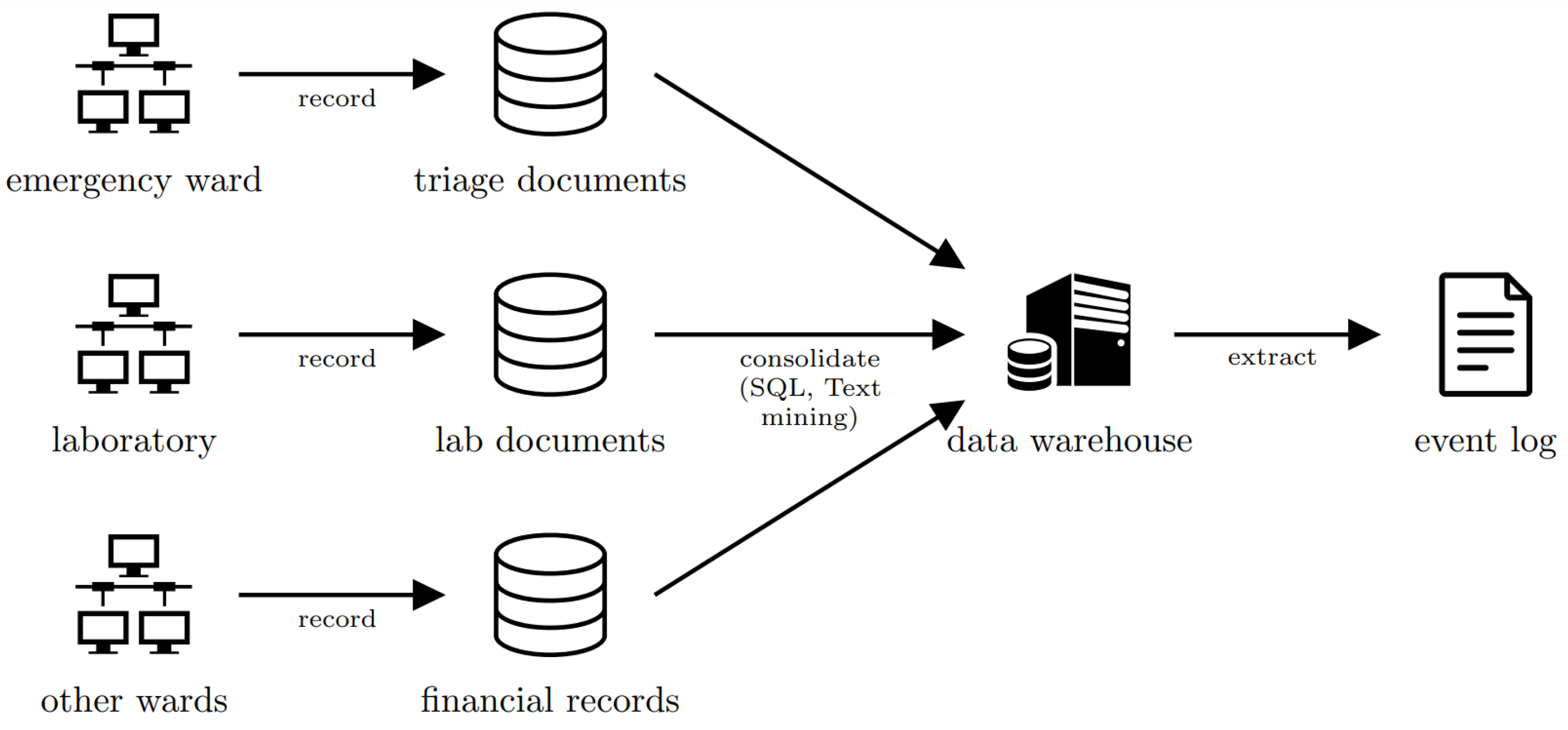
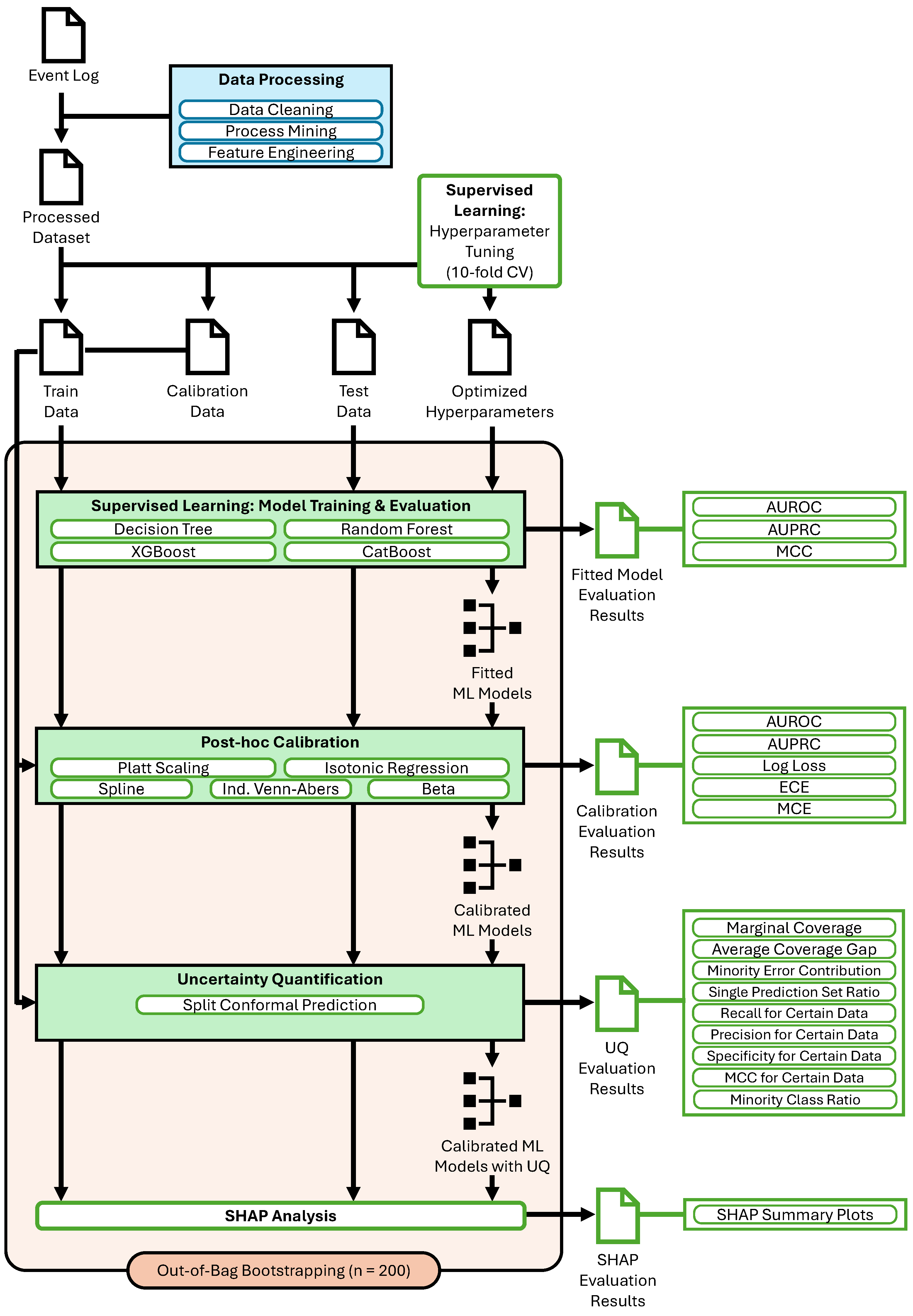
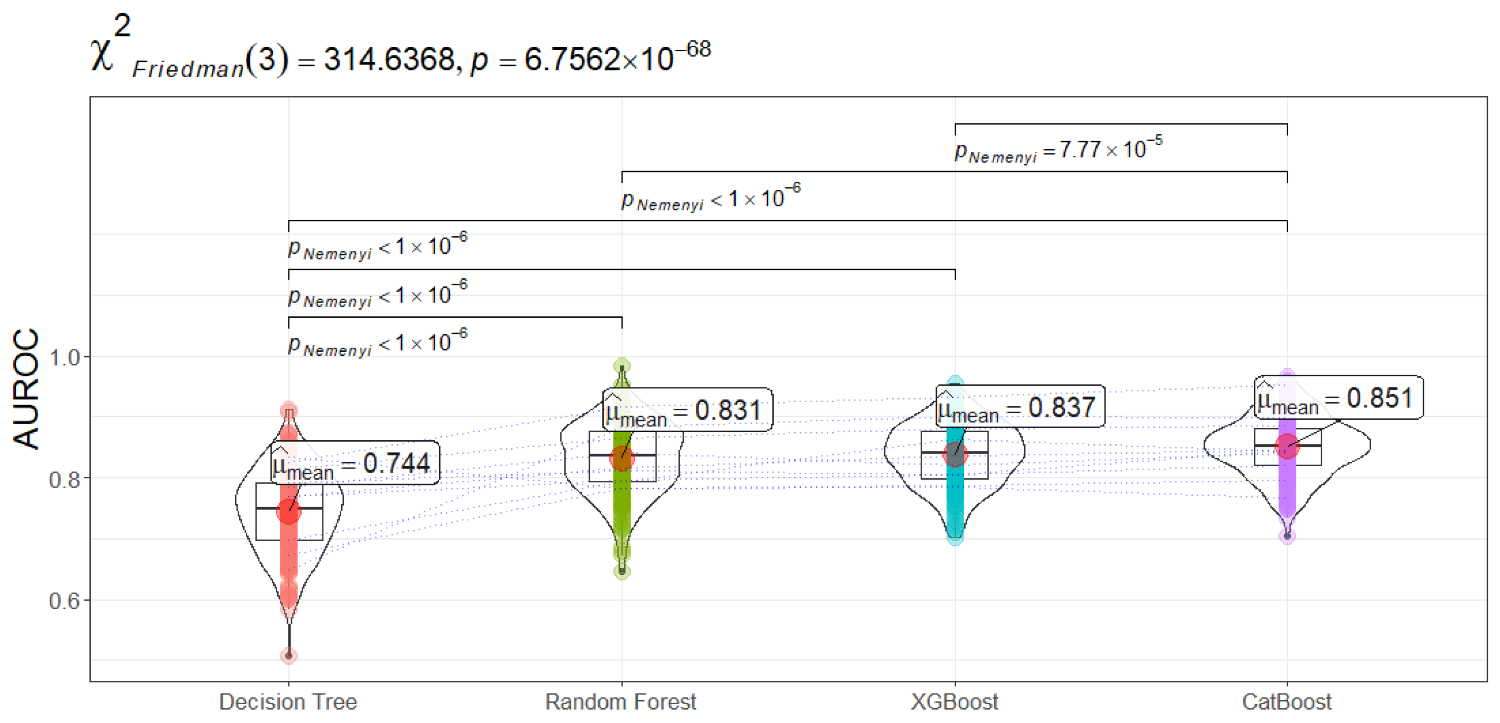
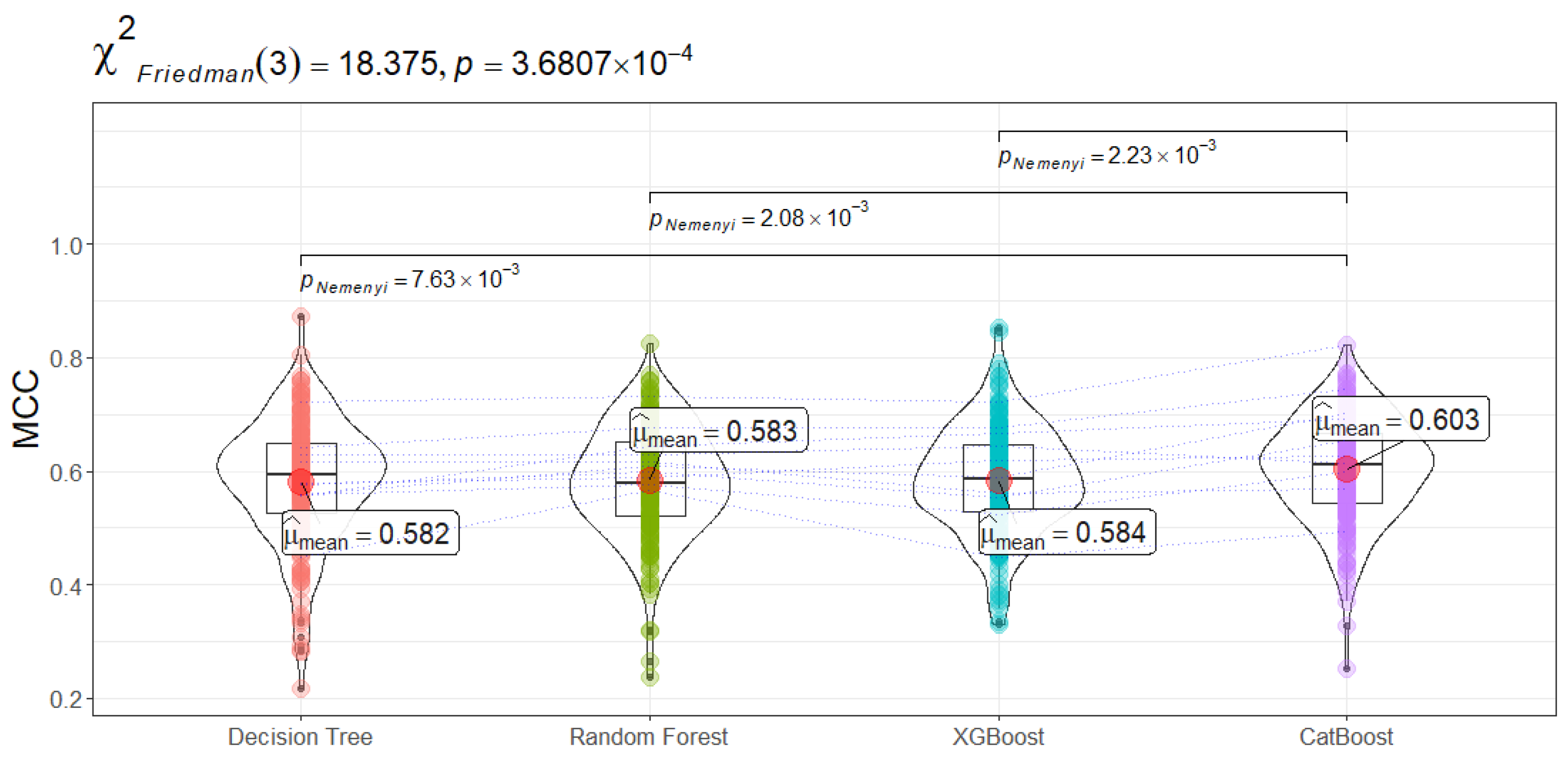
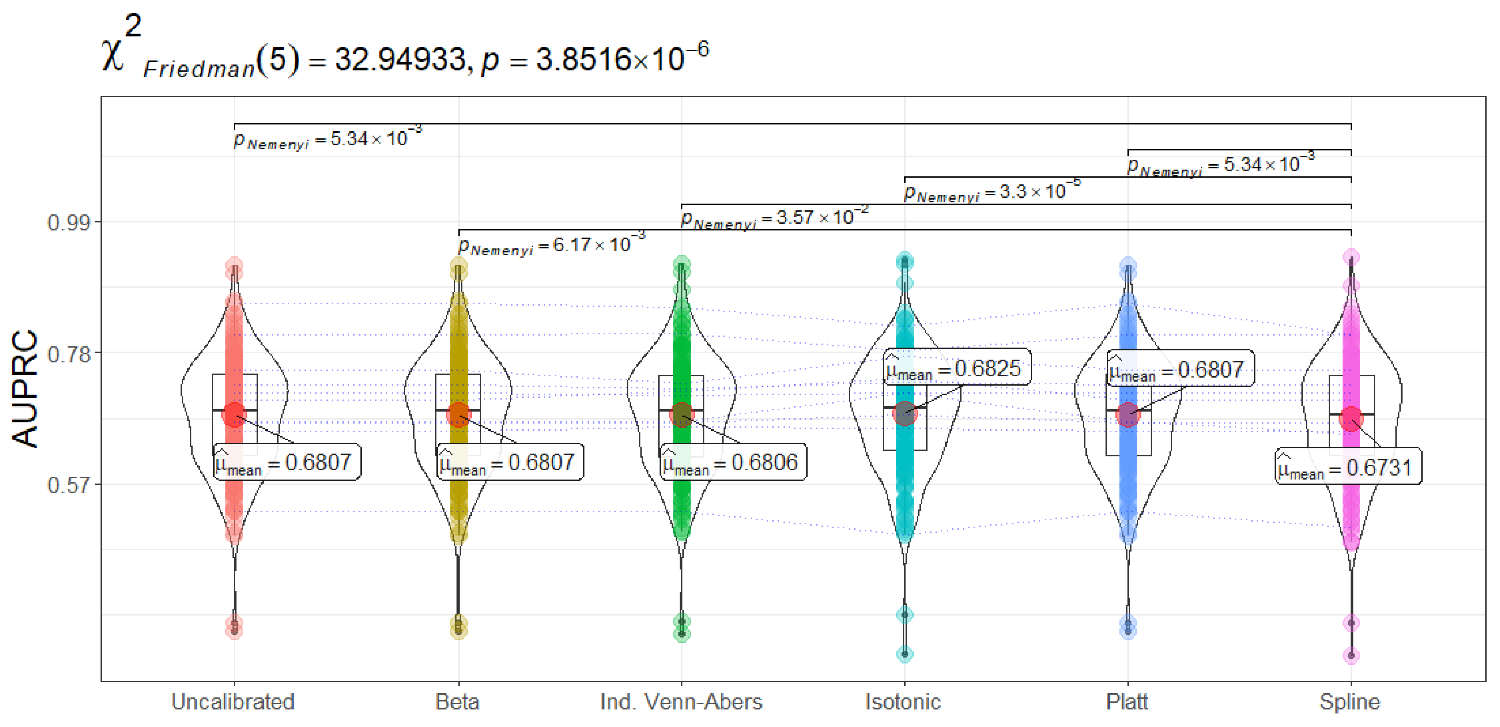
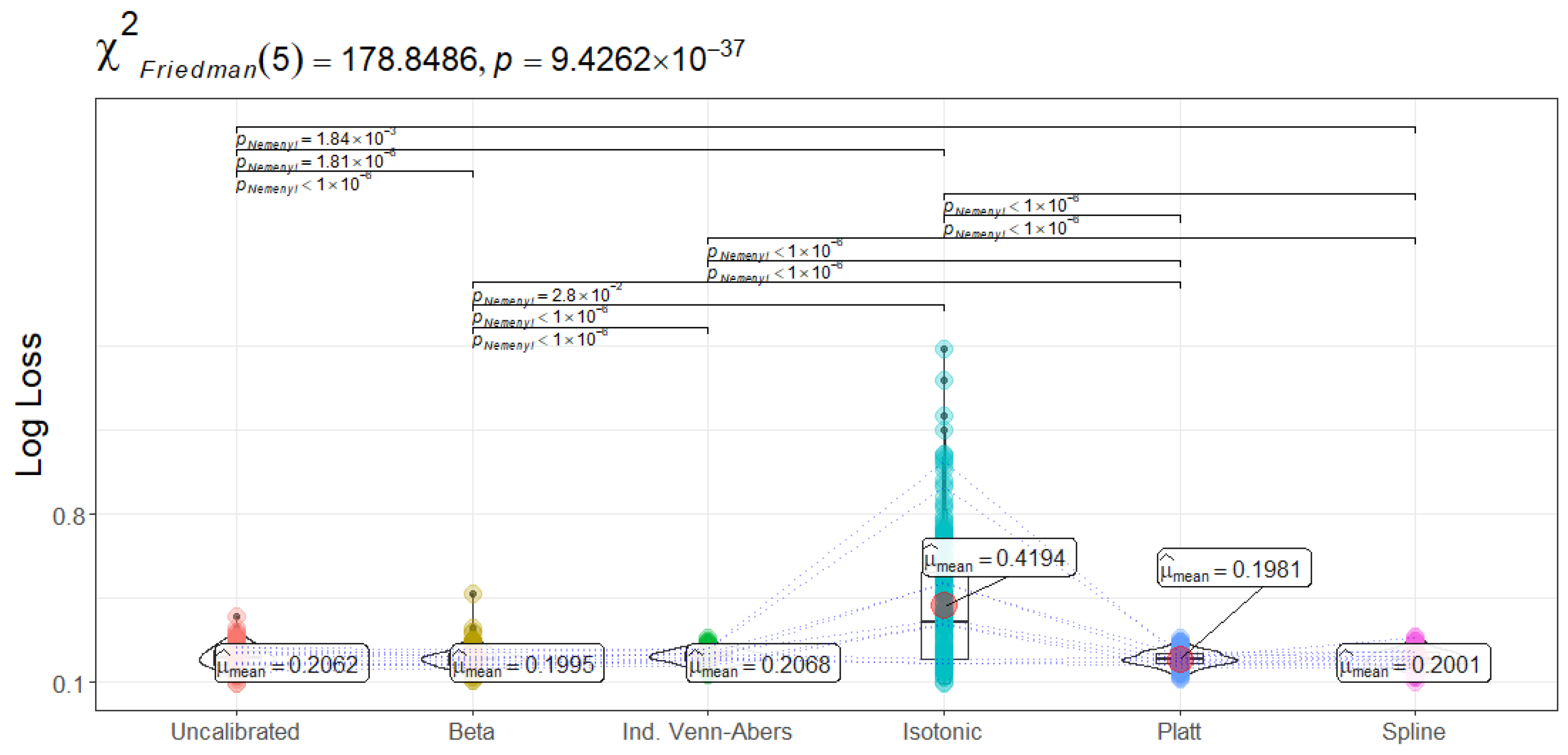
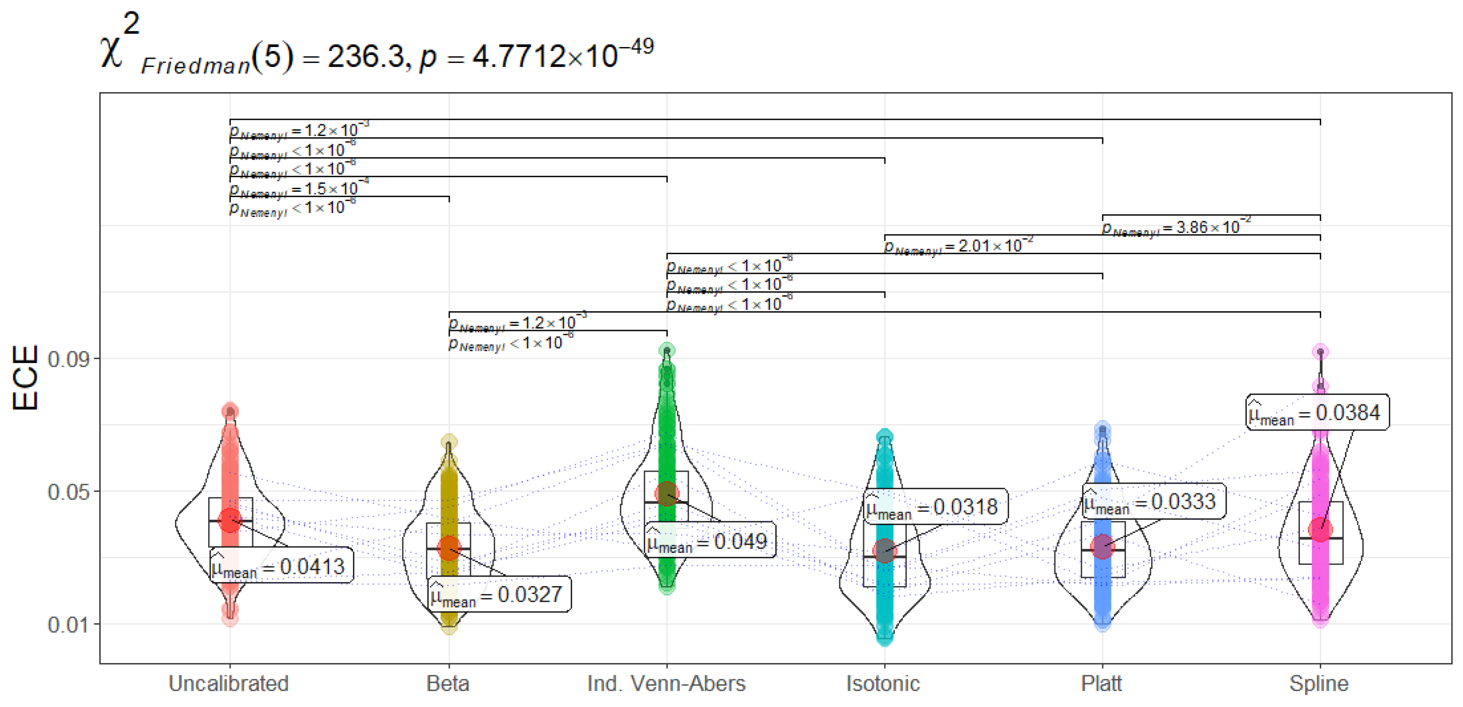
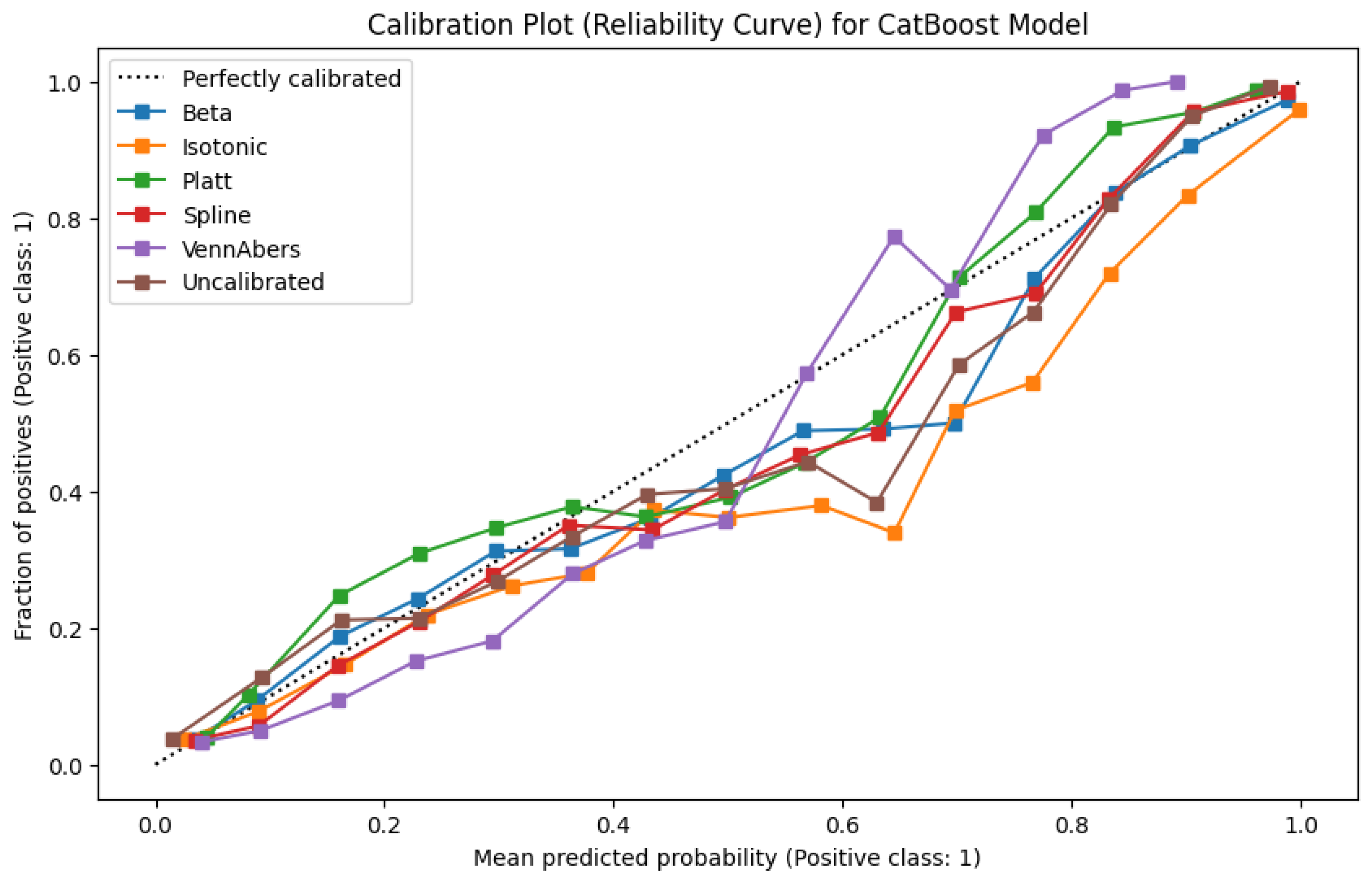
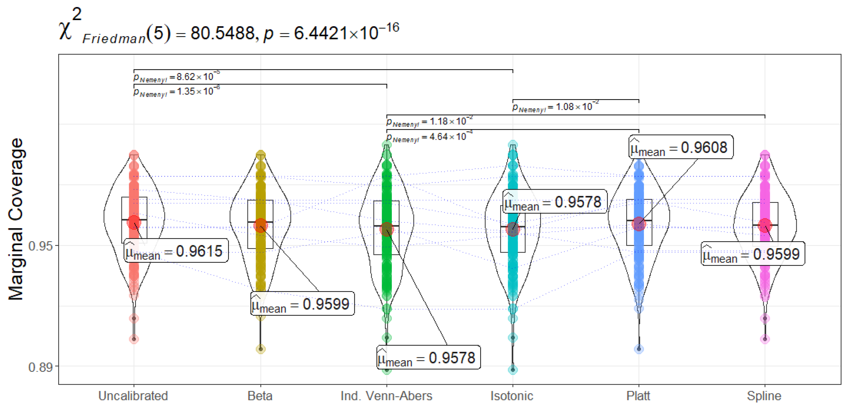
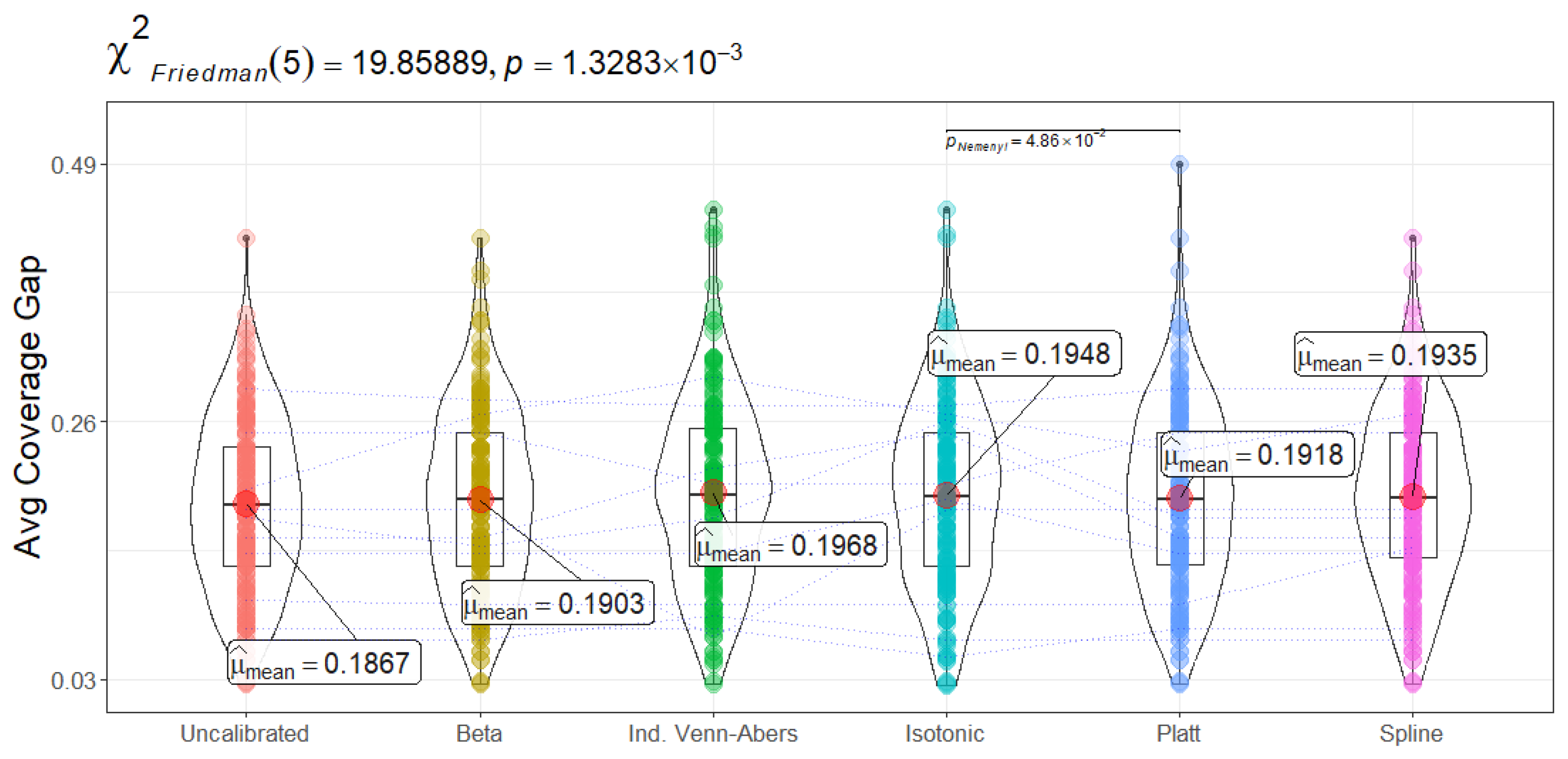
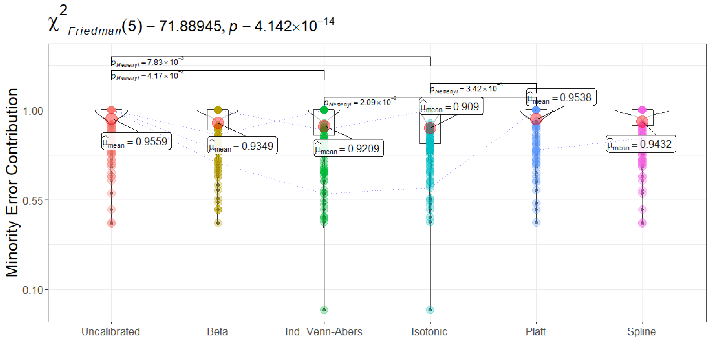
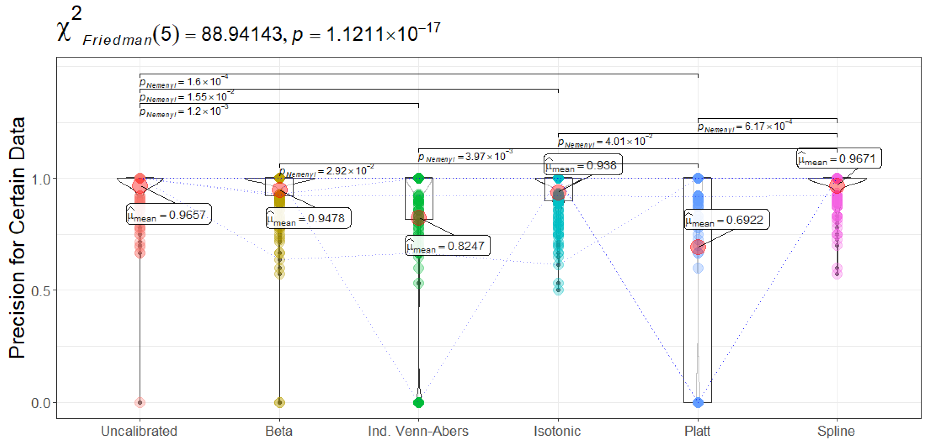
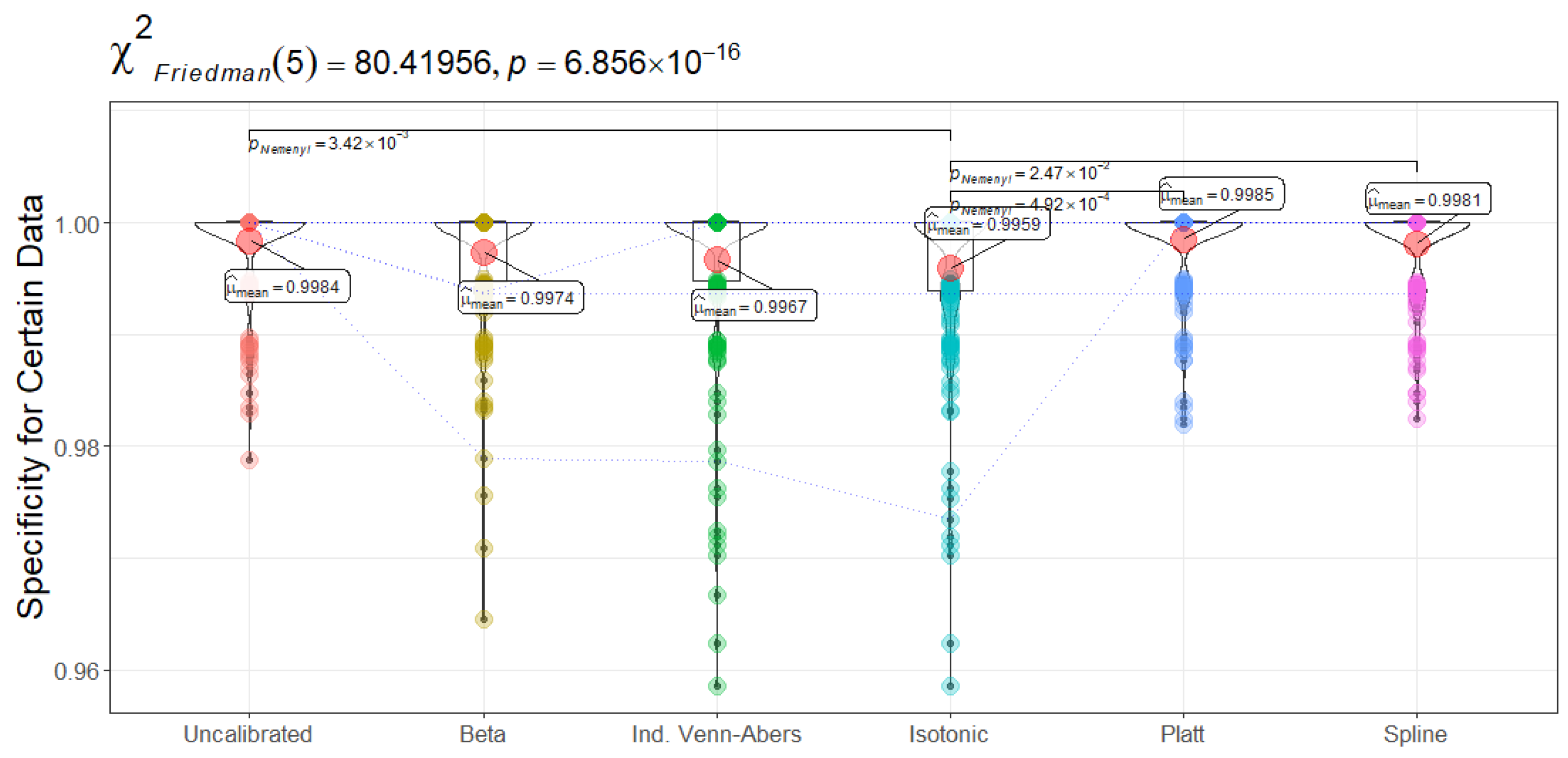
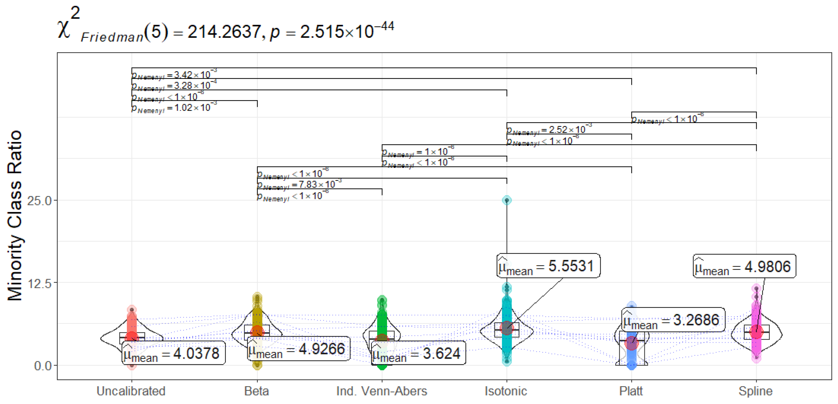
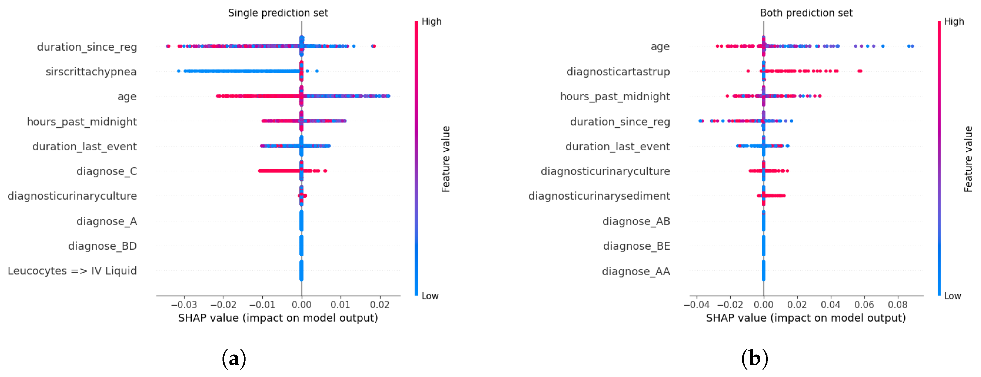
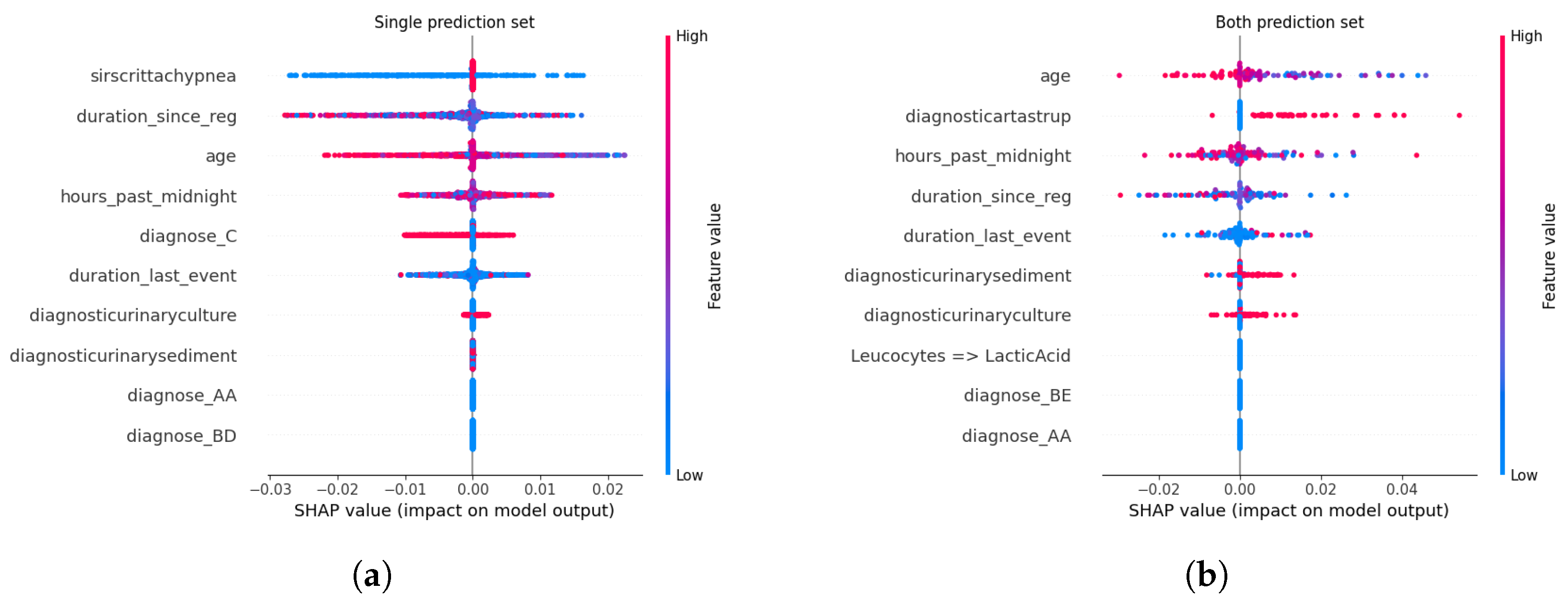
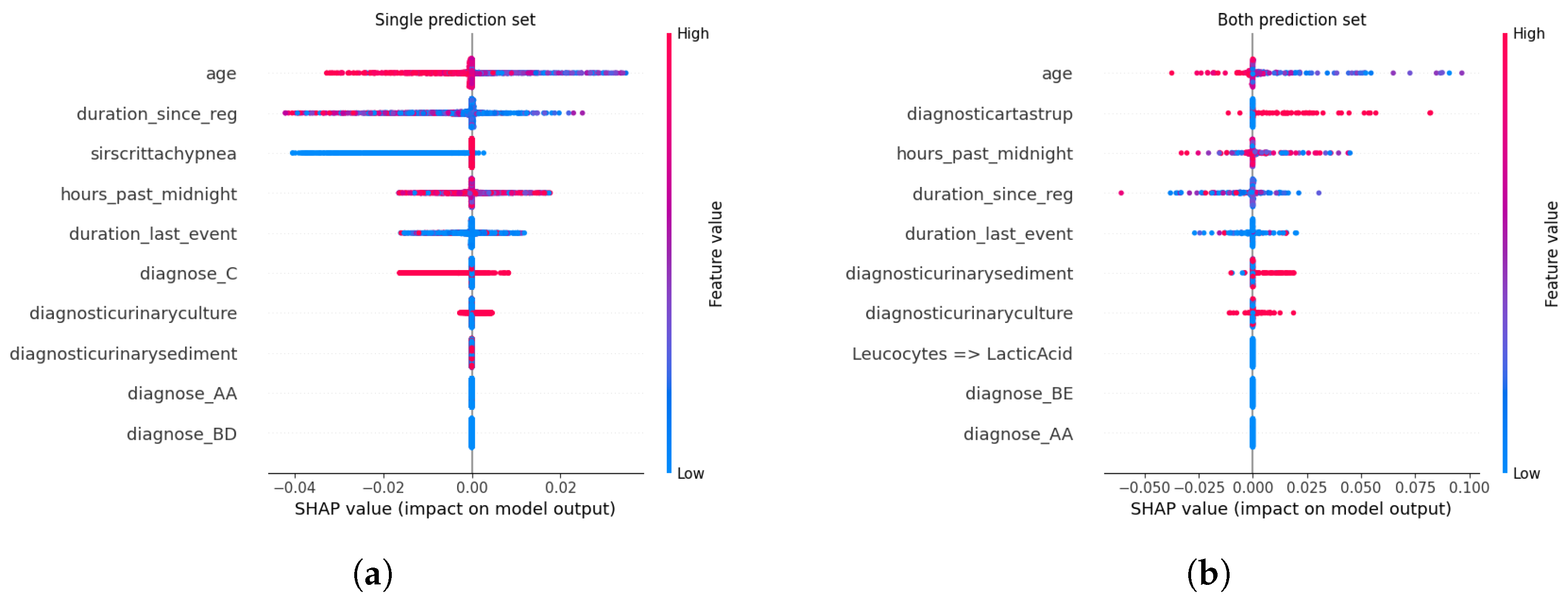
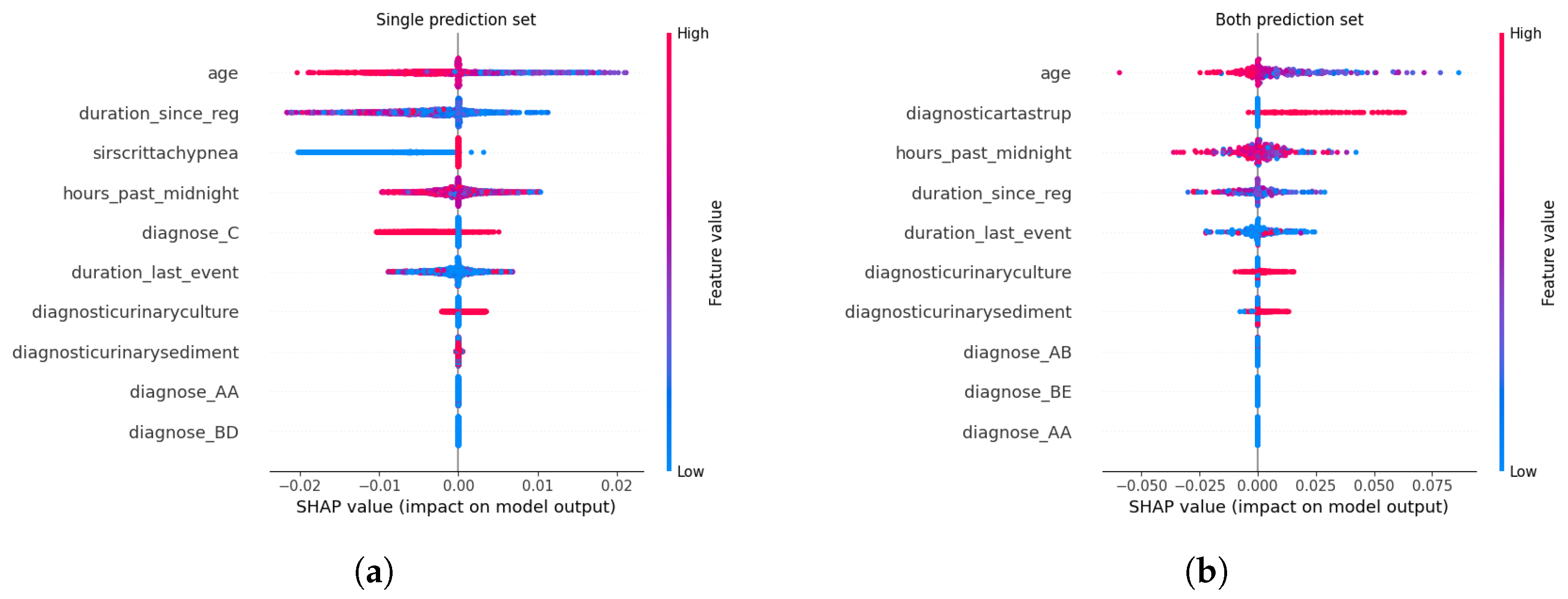
8. Conclusions

In summary, our study demonstrates that integrating probability calibration techniques with CP framework enhances both the statistical robustness and interpretability of PPM in high-stakes healthcare applications. By systematically comparing post-hoc calibration methods we established that calibrated probabilities not only align better with empirical outcomes but also improve the reliability of uncertainty estimates generated via SPC. The experimental results indicate that while uncalibrated models can achieve high overall discrimination, they tend to misallocate uncertainty, particularly for the minority class. In contrast, calibration methods preserve classification performance while yielding lower log loss and improved ECE. Furthermore, explainability analysis based on SHAP values revealed that the calibration process reshapes feature attributions; non-parametric approaches, for instance, tie uncertainty more directly to clinically meaningful markers, thereby enhancing model transparency and fostering clinician trust. These findings highlight that calibration is not merely a technical adjustment but a transformative layer that influences model reasoning and uncertainty quantification.