Identification of Complicated Lithology with Machine Learning

Abstract

Lithology identification is one of the most important research areas in petroleum engineering, including reservoir characterization, formation evaluation, and reservoir modeling. Due to the complex structural environment, diverse lithofacies types, and differences in logging data and core data recording standards, there is significant overlap in the logging responses between different lithologies in the second member of the Lucaogou Formation in the Santanghu Basin. Machine learning methods have demonstrated powerful nonlinear capabilities that have a strong advantage in addressing complex nonlinear relationships between data. In this paper, based on felsic content, the lithologies in the study area are classified into four categories from high to low: tuff, dolomitic tuff, tuffaceous dolomite, and dolomite. We also study select logging attributes that are sensitive to lithology, such as natural gamma, acoustic travel time, neutron, and compensated density. Using machine learning methods, XGBoost, random forest, and support vector regression were selected to conduct lithology identification and favorable reservoir prediction in the study. The prediction results show that when trained with 80% of the predictors, the prediction performance of all three models has improved to varying degrees. Among them, Random Forest performed best in predicting felsic content, with an MAE of 0.11, an MSE of 0.020, an RMSE of 0.14, and a R² of 0.43. XGBoost ranked second, with an MAE of 0.12, an MSE of 0.022, an RMSE of 0.15, and an R² of 0.42. SVR performed the poorest. By comparing the actual core data with the predicted data, it was found that the results are relatively close to the XRD results, indicating that the prediction accuracy is high.

1. Introduction

In the process of well logging reservoir evaluation, lithology identification plays a crucial role. Coring in drilling is the most reliable technique for lithology identification. However, due to the high costs and limitations on core recovery rates, it is generally not feasible to core all intervals of a well. In this case, relying on well logging data for lithology analysis has become a critical technical approach. Currently, traditional methods and intelligent recognition methods are the primary analytical tools [1].

Traditional methods include the chart method, qualitative interpretation based on logging curves, and quantitative interpretation based on response equations. These largely rely on linear data and demonstrate limited capability in capturing the nonlinear relationships between logging parameters and lithology, especially under complex geological conditions. For instance, lithology identification models based on probabilistic and statistical analysis often depend heavily on prior information and are highly sensitive to assumptions about data distribution. Similarly, the crossplot method analyzes two-dimensional or three-dimensional intersections of logging parameters, but it relies strongly on the empirical judgment of geological experts and performs poorly in complex lithological transition zones. To sum up, these methods have significant limitations when identifying complex carbonate lithologies, and most can only distinguish a limited number of lithologies, including limestone and dolomite [2,3,4].

Due to the rapid development of machine learning technology, intelligent machine learning methods have been widely applied in lithology identification. Many scholars have used support vector machines [5,6], neural networks [7,8,9], fuzzy recognition [10,11], and traditional decision tree methods [12,13,14] to classify and identify complex carbonate rock lithology and carbonate rock diagenetic facies. These methods demonstrate advantages in handling large amounts of data and recognizing complex patterns, which helps improve the accuracy and efficiency of lithology identification [15]. Therefore, combining traditional logging interpretation methods with machine learning techniques can more effectively identify complex carbonate rock lithology, providing more accurate information for logging reservoir evaluation.

Zhao Jian et al. (2003) [16] utilized density, resistivity, and gamma-ray logging curves to identify lithology in an operational area by analyzing the corresponding logging curve response characteristics in their study of the Songliao Basin in China. Subsequently, Zhang Daquan et al. [17], through core analysis, selected optimal logging curves and established crossplots, which greatly enhanced the identification of lithology in the Junggar area. Following this, other scholars have also applied similar methods in their research. For example, Pang et al. [18] observed core samples, conducted classification, and then used logging curve crossplots, ultimately achieving lithology identification.

The crossplot method is an important technique in geophysical logging, primarily used for lithology identification and interpretation. This method involves using two or more logging parameters (natural gamma ray, resistivity, acoustic transit time, etc.) as the axes to plot a crossplot on a plane. This allows for a visual representation of the characteristics and differences in logging responses for different lithologies or formations [19]. Therefore, the crossplot method is one of the most commonly used methods in lithology identification.

The crossplot method is effective when the lithology is relatively simple and the corresponding features of the logging curves show significant differences. However, when the lithology becomes complex and the differences in the logging curve characteristics of the rocks are not pronounced, it becomes difficult to achieve effective results. In order to deal with this issue, some scholars have proposed using statistical methods for lithology identification. This approach involves organizing and summarizing observational data, followed by classification, to overcome the limitations of the crossplot method. The mathematical and statistical method was first proposed by Delfiner [20], and later, J.M. Busch and others applied this method in practical production, thoroughly demonstrating its feasibility and effectiveness. This method was later introduced to China, where domestic scholars conducted extensive research. Liu Ziyun et al. [21] designed a corresponding program based on this method for lithology identification in the North China region. In 2007, Liu et al. [22] developed a lithology identification model suitable for the study area using multivariate statistical methods. Practical verification has revealed that the multiple discriminant method can effectively identify lithology in most cases. However, it has significant errors when identifying lithology in transitional layers. Therefore, this method is not suitable when the geological features and lithology are complex. Based on the research progress of scholars both domestically and internationally, the mathematical and statistical method still relies heavily on expert experience. However, with the continuous development of computer technology, artificial intelligence has become increasingly complementary to this approach. Combining mathematical and statistical methods with AI for lithology identification has also become a popular research area [23].

In 2013, Wang et al. [24] compared the application effects of neural network and vector machine models and concluded that combining machine learning methods with other optimization algorithms could achieve lower computational costs and better stability. Later, Bhattacharya et al. [25] further validated this by comparing the performance of support vector machines, artificial neural networks, self-organizing maps, and multi-resolution graph-based clustering algorithms in shale lithology identification. They demonstrated that the vector machine outperformed other methods in lithology classification and identification.

In a global machine learning competition organized by Brendon Hall [26], participating teams used various machine learning algorithms for lithology identification. The comparison revealed that the XGBoost algorithm achieved the highest accuracy in lithology classification and identification. Zhou et al. [27] applied the rough set–random forest algorithm to train logging data and sample data, establishing a corresponding discriminant model. This approach was proven to have high accuracy in lithology identification. In 2018, An Peng et al. [28] based their work on the TensorFlow deep learning framework, integrating various techniques such as the Adagrad optimization algorithm, ReLU activation function, and Softmax regression layer into a neural network model. After training with sample data, this model demonstrated extremely high accuracy in conventional lithology identification. In 2019, Yadigar Imamverdiyev et al. [29] developed a one-dimensional convolutional neural network model. Compared to other machine learning methods, this model provided more accurate lithology classification predictions and also performed well in areas with complex geological structures. Chen et al. [30] applied convolutional neural networks to a specific study area and ultimately achieved very promising results. This paper utilizes machine learning methods, employing artificial intelligence for nonlinear prediction, to predict felsic content using logging data. Through research and analysis, three suitable machine learning methods were selected: XGBoost, random forest, and support vector regression. The predicted felsic content, along with the existing TOC content, was used for lithology identification and to predict favorable reservoirs.

2. Model Principles

2.1. Decision Tree and Random Forest Algorithm Principles

The structure of a decision tree consists of several key elements, including the root node, which serves as the starting point of the tree; branches that represent the decision paths; and leaf nodes that indicate the final prediction outcomes. The root node, located at the beginning of the decision tree, serves as the starting point of the entire tree structure. Each branch represents the path leading to a new decision point or a leaf node. Each decision node reflects a specific objective or requirement, usually associated with the characteristics of the target instances. The leaf nodes represent the predicted values derived within a specific range. When traversing the decision tree, the process begins at the root node and moves downward step by step. At each node, a prediction is made, and based on the different prediction outcomes, the path continues along the corresponding branch until it reaches a leaf node. This process embodies the core of the decision tree algorithm, which is to use multiple variables to perform classification prediction or regression analysis on the target. Figure 1 illustrates a simple conceptual diagram of the decision tree principle.

Random forest (RF) is an ensemble learning method that improves prediction accuracy and stability by constructing multiple decision trees and integrating their results. This method introduces two main types of randomness when building each decision tree: first, by using bootstrap sampling to generate multiple different training subsets from the original dataset, it ensures that each tree is trained on a different subset of data; second, at each split node, a random subset of features is selected as candidate features, and the best feature is chosen from this subset to perform the split. This further increases diversity among the trees [31]. The final prediction of the random forest is obtained by aggregating the results of multiple decision trees. For classification problems, the majority voting method is typically used; for regression problems, the average of all the trees’ predicted results is calculated as the final output. The advantage of this method lies in its ability to provide high prediction accuracy while effectively resisting overfitting.

2.2. Support Vector Machine Algorithm Principles

Support vector machine (SVM) is a powerful supervised learning model primarily used for classification problems. Its core principle is to find an optimal hyperplane in a high-dimensional space that maximizes the margin between the data points of different classes. The support vectors are the data points closest to this hyperplane, and they determine the position and orientation of the hyperplane [32].

When selecting an appropriate kernel function, the following empirical guidelines are typically followed: If the dataset has a large number of features with high dimensionality, and the data points can be linearly separated, a linear kernel or polynomial kernel is a suitable choice. For such datasets, especially when the number of features far exceeds the number of samples, a linear or polynomial kernel often yields good results. Additionally, these kernels generally perform faster during training compared to other nonlinear kernels. Conversely, when the input data has lower dimensionality and a small sample size, and the data exhibits significant nonlinear characteristics, the Gaussian kernel (a type of radial basis function) is particularly well suited for handling nonlinear problems. Similarly, the sigmoid kernel function is also applicable to datasets with nonlinear characteristics. Although it is not as flexible as the Gaussian kernel, the sigmoid kernel tends to perform better in terms of generalization on unseen data, which helps prevent the model from overfitting [33].

Commonly used kernel functions include

$$linear,k\left(x,y\right)=x^{\prime }\ast y$$

(1)

$$poly,k\left(x,y\right)={\left(x^{\prime }\ast y+c\right)}^d$$

(2)

$$gauss,k\left(x,y\right)=\exp \left(-0.5\ast {\left({\displaystyle \frac{norm\left(x-y\right)}{s}}\right)}^2\right)$$

(3)

$$sigmoid,k\left(x,y\right)=\tanh \left(g\ast x^{\prime }\ast y+c\right)$$

(4)

When applied to regression, the variant of support vector machine (SVM) is called support vector regression (SVR). The goal of SVR is to find a function that ensures the predicted values are as close as possible to the actual data points within a given tolerance range. The main difference between SVR and SVM is that in SVR, there is no need to classify samples. The objective is not to find an optimal hyperplane that maximizes the distance between all sample points, as in SVM, but rather to find a hyperplane that brings all sample points as close as possible to it. In SVR, the sample points are located between two tolerance lines, with the distance between these lines and the hyperplane representing a predetermined threshold. This kind of hyperplane minimizes the regression error, similar to the margin maximization in SVM [34].

2.3. XGBoost Algorithm Principles

XGBoost is essentially a type of Gradient-Boosting Decision Tree (GBDT) but with enhancements in speed and efficiency, hence the term “Extreme Boosted”. Its core idea involves the introduction of a regularization term and the optimization of the loss function using both first-order and second-order derivatives. XGBoost supports various types of base classifiers, allows for data sampling, and can handle missing values. XGBoost is an iterative decision tree algorithm that falls under the category of ensemble learning algorithms. Its core idea is to calculate the residuals between the model’s predicted values and the actual values during multiple iterations and then use these residuals as new target variables for training. Through continuous iteration, a strong classifier is formed. As the number of iterations increases, the prediction results of the ensemble classifier become more accurate [35,36]. XGBoost gradually reduces prediction errors by iteratively generating CART trees, thereby improving prediction accuracy. The XGBoost algorithm is illustrated in Figure 2.

3. Data Selection and Practical Application

3.1. Analysis of the Relationship Between Logging Parameters and Feldspar Content

(1)

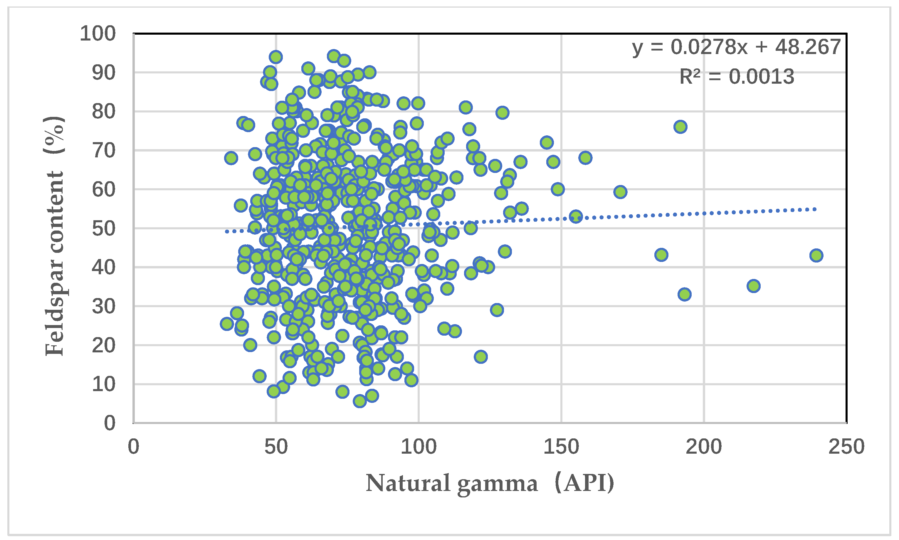
Intersection plot of natural gamma and feldspar content

Figure 3 depicts an intersection graph of natural gamma and feldspar content. It can be seen from the graph that natural gamma is positively correlated with feldspar content, but the correlation is extremely poor, with a correlation coefficient of only 0.001.

(2)

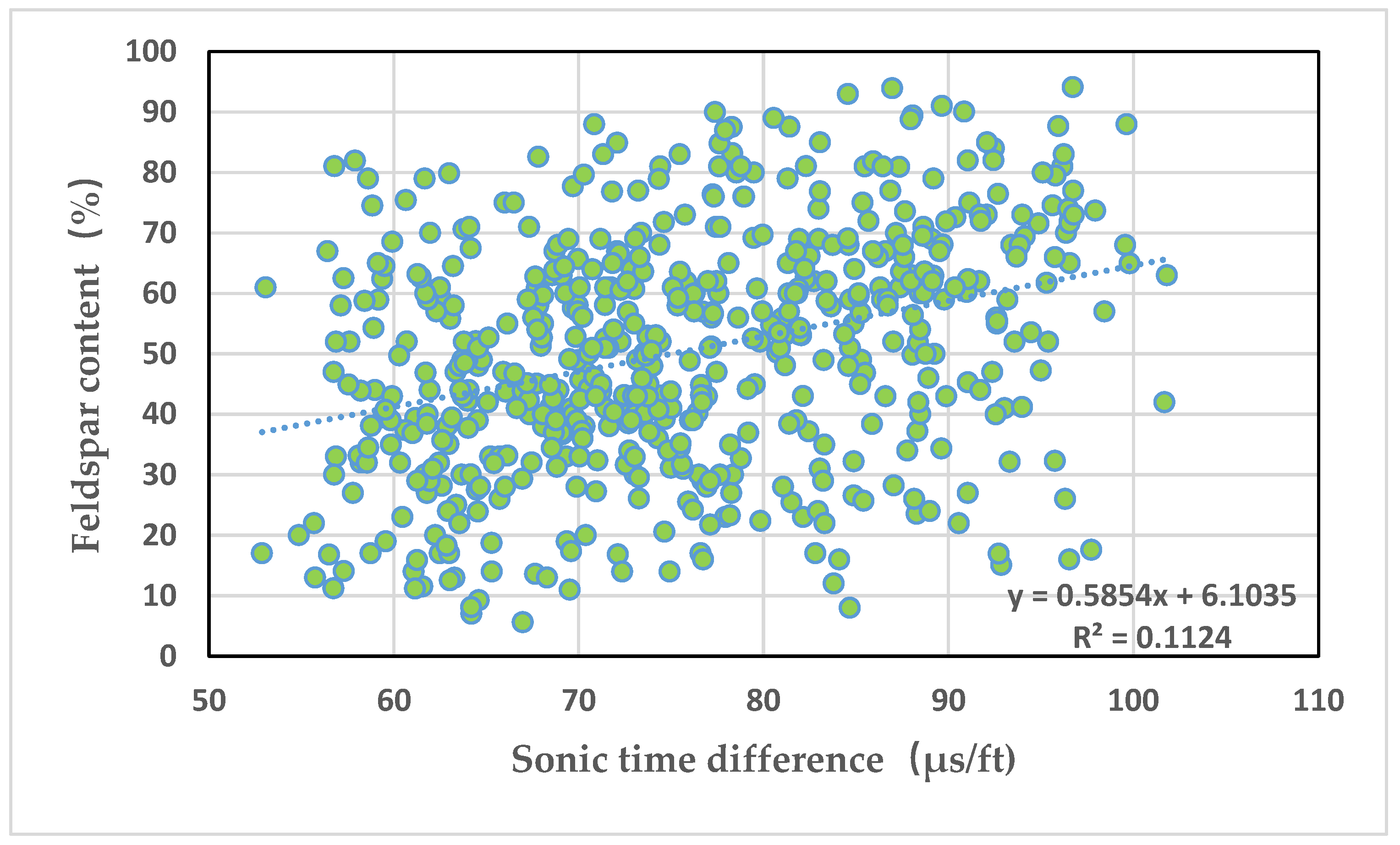
Intersection plot of acoustic time difference and long quartz content

Figure 4 depicts an intersection graph of the time difference between sound waves and long quartz content. It can be seen from the graph that the time difference of sound waves is positively correlated with the long quartz content, but the correlation is poor, with a correlation coefficient of 0.112.

(3)

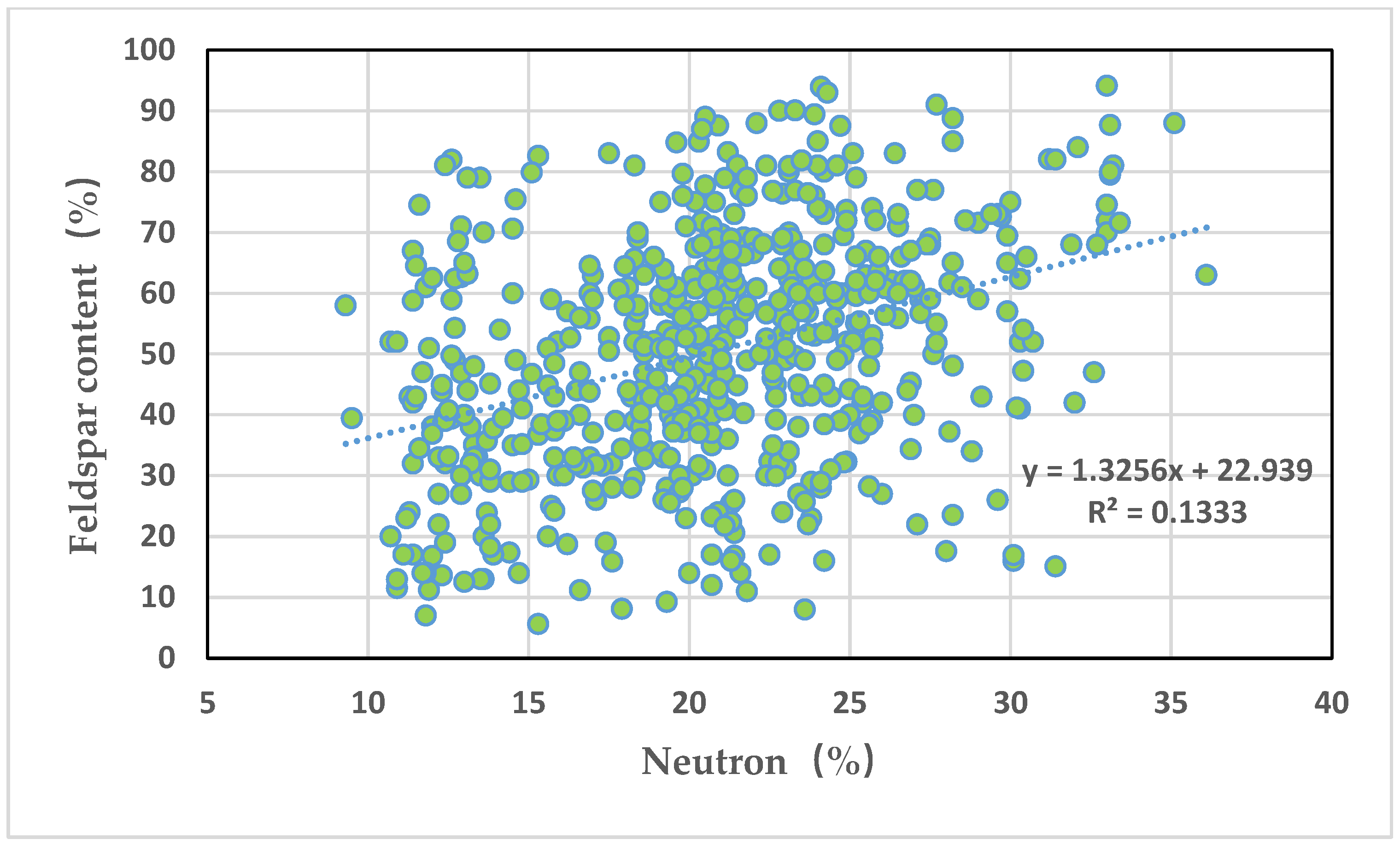
Intersection plot of neutron and long quartz content

Figure 5 depicts an intersection graph of neutron and long quartz content. It can be seen from the graph that neutron and long quartz content are positively correlated, but the correlation is poor, with a correlation coefficient of 0.133.

(4)

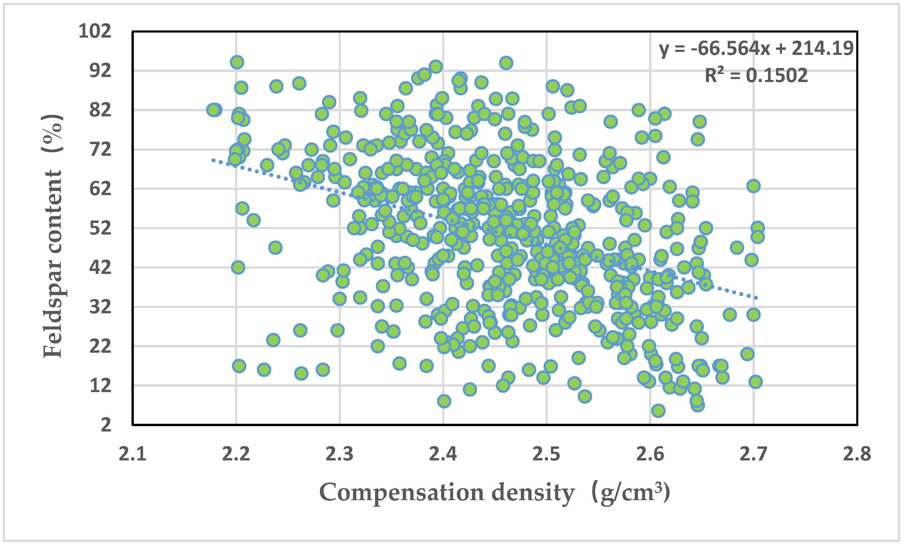
Intersection plot of compensation density and feldspar content

Figure 6 depicts an intersection graph of compensation density and feldspar content. It can be seen from the graph that the compensation density is positively correlated with the feldspar content, but the correlation is poor, with a correlation coefficient of 0.15.

(5)

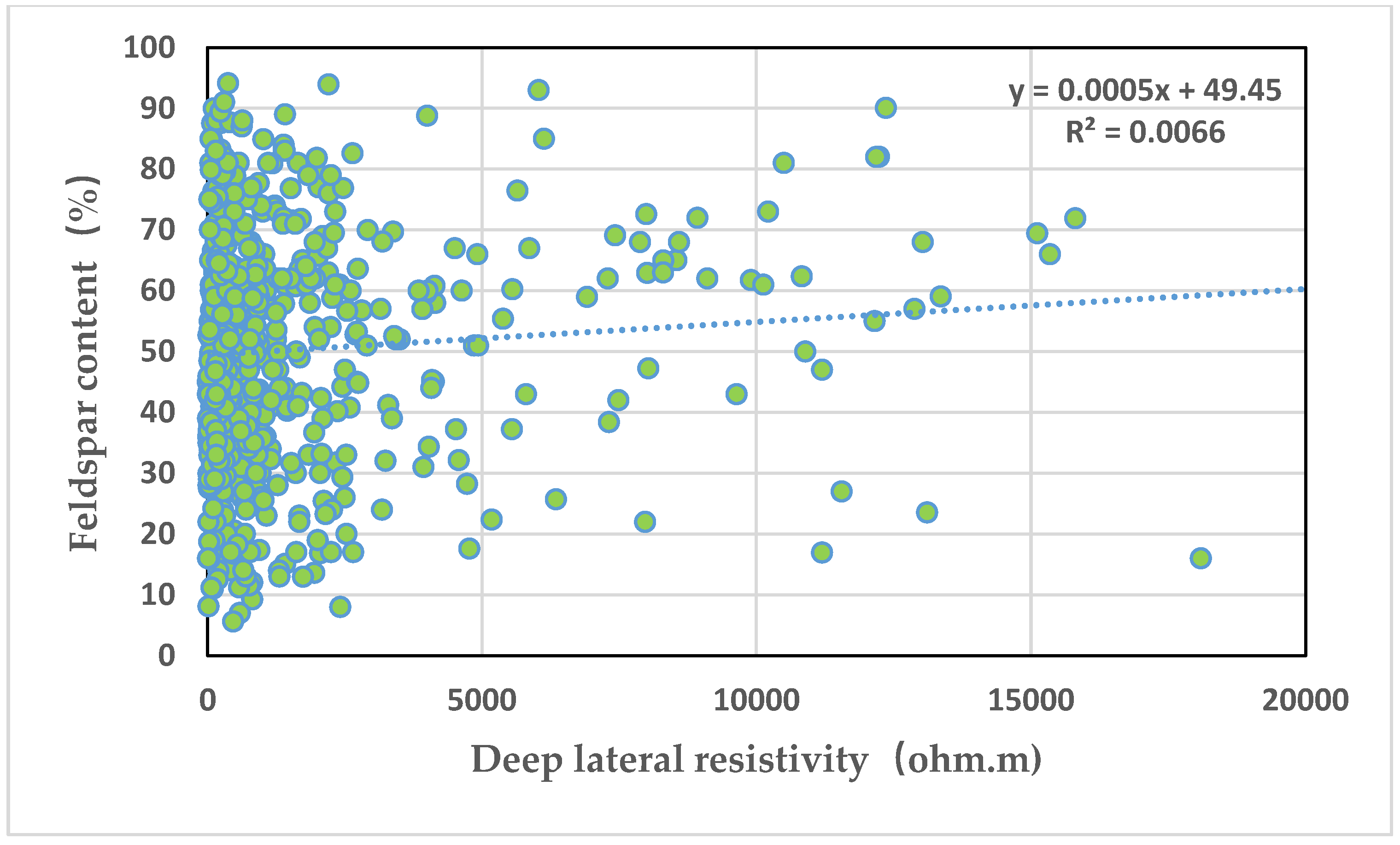
Intersection plot of deep lateral resistivity and feldspar content

Figure 7 depicts an intersection graph of deep lateral resistivity and long quartz content. It can be seen from the graph that deep lateral resistivity is positively correlated with long quartz content, but the correlation is extremely poor, with a correlation coefficient of 0.007.

(6)

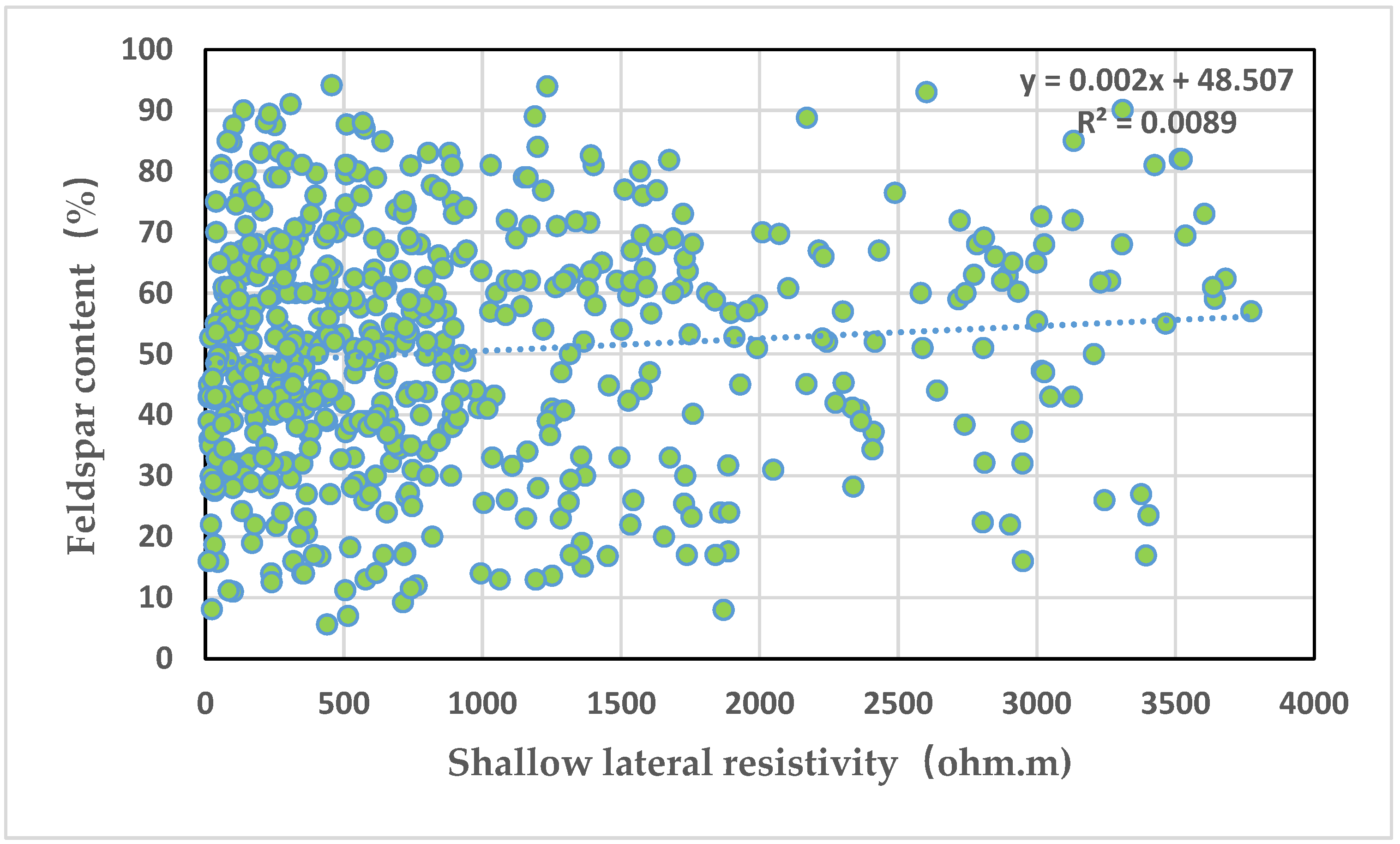
Intersection plot of shallow lateral resistivity and feldspar content

Figure 8 depicts an intersection graph of the shallow lateral resistivity and long quartz content. It can be seen from the graph that the deep lateral resistivity is positively correlated with the long quartz content, but the correlation is extremely poor, with a correlation coefficient of 0.009.

The existence of these correlations supports our decision to adopt machine learning algorithms that can handle moderate multicollinearity.

3.2. Data Preparation

The original felsic dataset in the study area contains 834 sample points. After data preprocessing, the number of sample points was reduced to 493. Two different data splits were chosen: 80% of the data was used as the training set, 20% as the test set, and vice versa—20% as the training set and 80% as the test set. In this paper, the characteristics of the model input were determined through principal component analysis and XGBoost feature importance analysis. The contribution results of these features, evaluated by principal component analysis (PCA), show that the first three principal components cumulatively explain approximately 97.67% of the total variance (

Table 1. Total variance interpretation table.

Component	Eigenvalue	Percentage of Variance	Cumulative Percentage
1	3.538	58.280	58.28
2	1.422	23.420	81.70
3	0.970	15.972	97.672
4	0.080	1.323	98.995
5	0.046	0.766	99.761
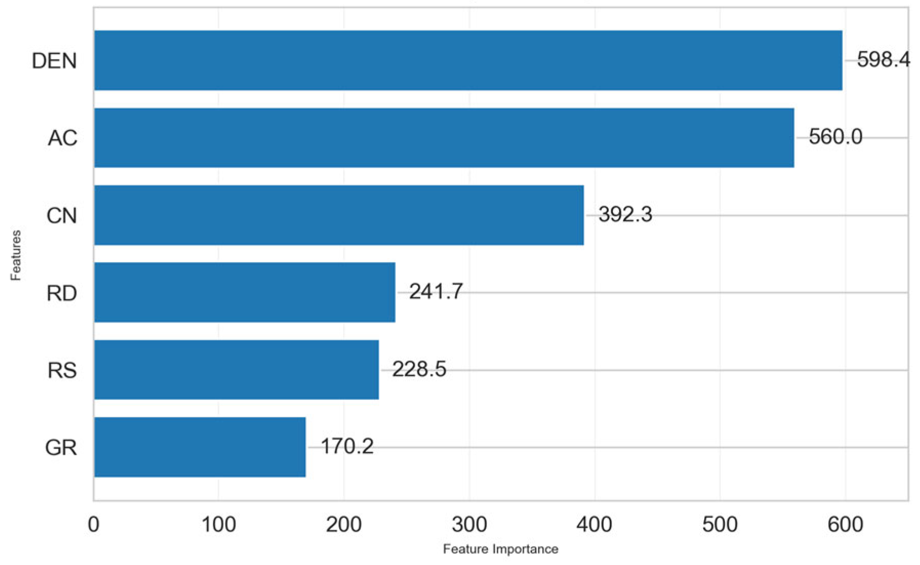
6	0.014	0.239	100.00

). However, considering the geological information represented by different features, XGBoost feature importance analysis was used simultaneously to confirm that each feature makes a unique contribution to the model (Figure 9). Finally, six input features of the model, namely, GR, AC, CN, DEN, RS, and RD, were determined. However, due to differences in the dimensions and value ranges among these logging curves, min–max normalization of the data was required before model training. The formula for min–max normalization is as follows:

$$Y={\displaystyle \frac{X-min}{max-min}}$$

(5)

In this context, Y represents the normalized data; X is the original data; and X_max and X_min are the maximum and minimum values of the logging parameter, respectively. After normalization, the data is transformed in a way that enhances the model’s ability to learn from the data effectively.

3.3. Model Evaluation

To compare the predictive performance of different models, this paper introduces several evaluation metrics, including Mean Absolute Error (MAE), Mean Squared Error (MSE), Root Mean Squared Error (RMSE), and the Coefficient of Determination (R-squared). These metrics are used to assess and contrast the accuracy and effectiveness of each model.

(1)

Mean Absolute Error (MAE): Also known as norm lossl_1, MAE is obtained by calculating the absolute difference between the predicted value and the actual value for each sample, summing these absolute differences, and then taking the average. The formula for MAE is shown in Equation (6).

$$MAE\left(y,\widehat{y}\right)={\displaystyle \frac{1}{n_{samples}}}\sum _{i=1}^{n_{samples}}\left|y_i-{\widehat{y}}_i\right|$$

(6)

MAE is the simplest evaluation metric in regression problems, primarily used to assess the closeness between predicted values and actual values. Its value is negatively correlated with the effectiveness of the regression; a lower MAE indicates better regression performance.

(2)

Mean Squared Error (MSE): Also known as norm lossl_2, MSE is calculated by taking the difference between each predicted value and the actual value, squaring this difference, summing all the squared differences, and then taking the average. The formula for MSE is shown in Equation (7).

$$MSE\left(y,\widehat{y}\right)={\displaystyle \frac{1}{n_{samples}}}\sum _{i=1}^{n_{samples}}{\left(y_i-{\widehat{y}}_i\right)}^2$$

(7)

MSE is calculated as the average of the squared differences between the predicted values and the actual values. Its value is negatively correlated with the effectiveness of the regression; a lower MSE indicates better regression performance.

(3)

Root Mean Squared Error (RMSE): RMSE is obtained by taking the square root of the Mean Squared Error (MSE). The formula for RMSE is shown in Equation (8).

$$RMSE\left(y,\widehat{y}\right)=\sqrt{{\displaystyle \frac{1}{n_{samples}}}\sum _{i=1}^{n_{samples}}{\left(y_i-{\widehat{y}}_i\right)}^2}$$

(8)

Similar to MSE, RMSE is negatively correlated with the effectiveness of the regression; a lower RMSE indicates better regression performance. RMSE addresses the issue of unit inconsistency between input and output that exists with MSE, but it still does not perform well in the presence of outliers.

(4)

Coefficient of Determination (R²): The coefficient of determination, also known as the R² score, reflects the proportion of the variance in the dependent variable that is predictable from the independent variables. As the goodness of fit of the regression model increases, the explanatory power of the independent variables over the dependent variable also increases, causing the actual observation points to cluster more closely around the regression line. The formula for R² is shown in Equation (9).

$$R^2\left(y,\widehat{y}\right)=1-{\displaystyle \frac{{\sum }_{i=1}^{n_{samples}}{\left(y_i-{\widehat{y}}_i\right)}^2}{{\sum }_{i=1}^{n_{samples}}{\left(y_i-{\stackrel{-}{y}}_i\right)}^2}}$$

(9)

In the formula ${\stackrel{-}{y}}_i={\displaystyle \frac{1}{n_{samples}}}{\sum }_{i=1}^{n_{samples}}{y}_i$, the value of R² ranges from 0 to 1, where a value closer to 1 indicates the better predictive performance of the model, and a value closer to 0 indicates poorer performance. It is also possible for R² to be negative, which indicates that the model performs extremely poorly. As the number of input features increases, the R² value will gradually stabilize at a constant value, at which point, adding more input features will no longer have a significant impact on the model’s prediction accuracy, neither improving nor reducing its performance.

3.4. Model Construction

This study selects three machine learning algorithms—random forest, support vector regression, and XGBoost—to predict felsic content in the study area. For the training dataset, two different ratios for the predictor variables and measured felsic content data were selected: 20% and 80%. After training the models, the remaining data was used as the validation set. The predictor variables in the validation set were then input into the models, and the felsic content was predicted using the three aforementioned machine learning methods.

For each machine learning algorithm adopted in this study, the grid search method was used to determine the hyperparameters of the model. For the XGBoost model, grid search explored the learning rate [0.01, 0.1, 0.2], the maximum tree depth [3, 5, 7], the number of estimators [50, 100, 200], the column sampling rate [0.3, 0.5, 0.8], and the regularized alpha value [1, 5, 10]. For the random forest and support vector regression models, the hyperparameter optimization of the models is carried out in the same way. Finally, the support vector regression model adopted the radial basis function (RBF) as the kernel function and set the regularization parameter, C, to 12.53 and the epsilon value to 0.31. The XGBoost model sets the maximum depth of the tree to 3 to prevent overfitting. The learning rate was selected as 0.01, and 200 decision trees were used for integration simultaneously. In total, 50% of the features of each tree were randomly sampled, and an l1 regularization coefficient of 5 was applied. The random forest regression model consists of 179 decision trees. The maximum depth limit of each tree is five layers, and the minimum number of samples required for internal node splitting is four. The model sets the random seed to 42.

3.4.1. XGBoost Prediction of Felsic Content

Initially, we selected 20% of the predictive factors for training. After achieving the best training results, we input the predictive factors of the test set into the trained model to obtain the predicted results. The evaluation metrics of the predicted results are shown in

Table 2. XGBoost model of 20% of the training samples from Well Lu 1 predicting the felsic quality evaluation index.

	MAE	MSE	RMSE	R2
XGBoost	0.19	0.023	0.15	0.36

:

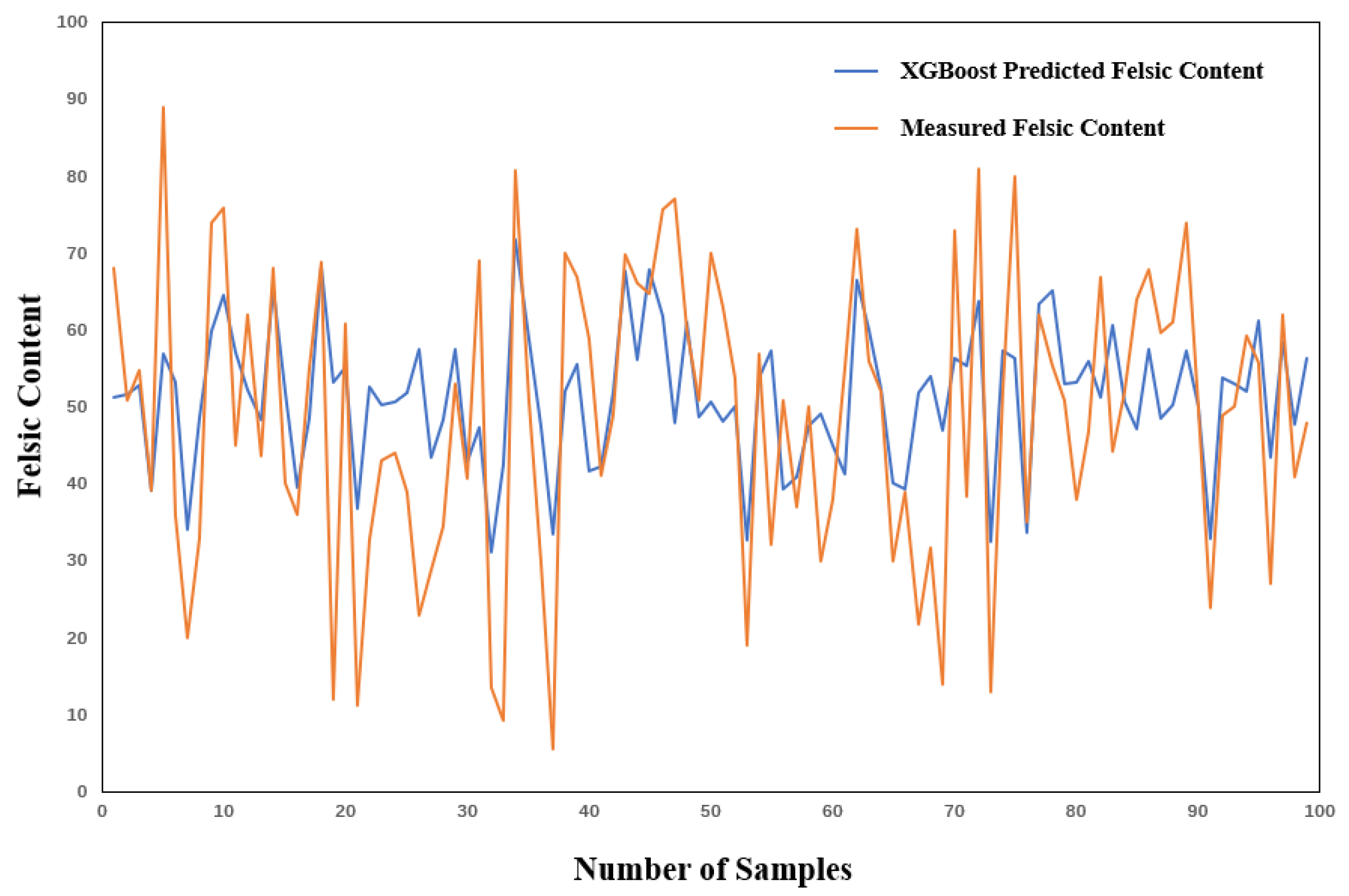
As shown in Table 2, when trained with 20% of the sample data, the MAE of the XGBoost model is 0.19, the MSE is 0.023, the RMSE is 0.15, and the R² is 0.36. These indicators reflect the initial predictive ability of the model. Among them, an R² of 0.36 indicates that the model can explain approximately 36% of the feldspar content, which is at a medium predictive level. An MAE value of 0.19 indicates that the average absolute error between the predicted value and the actual value is approximately 0.19, which still has considerable room for improvement in the prediction of feldspar content. The prediction results are shown in Figure 10.

As shown in Figure 10, the fluctuations of the values predicted by the XGBoost model are generally similar to those of the actual values, although there are significant differences between the predicted and actual values at some peaks and troughs. Subsequently, 80% of the predictive factors were selected for training. After achieving the best training results, the predictive factors of the test set were input into the trained model to obtain the predicted results. The evaluation metrics of the predicted results are shown in

Table 3. XGBoost model of 80% of the training samples in Well Lu 1 predicting the felsic evaluation index.

	MAE	MSE	RMSE	R2
XGBoost	0.12	0.022	0.15	0.42

:

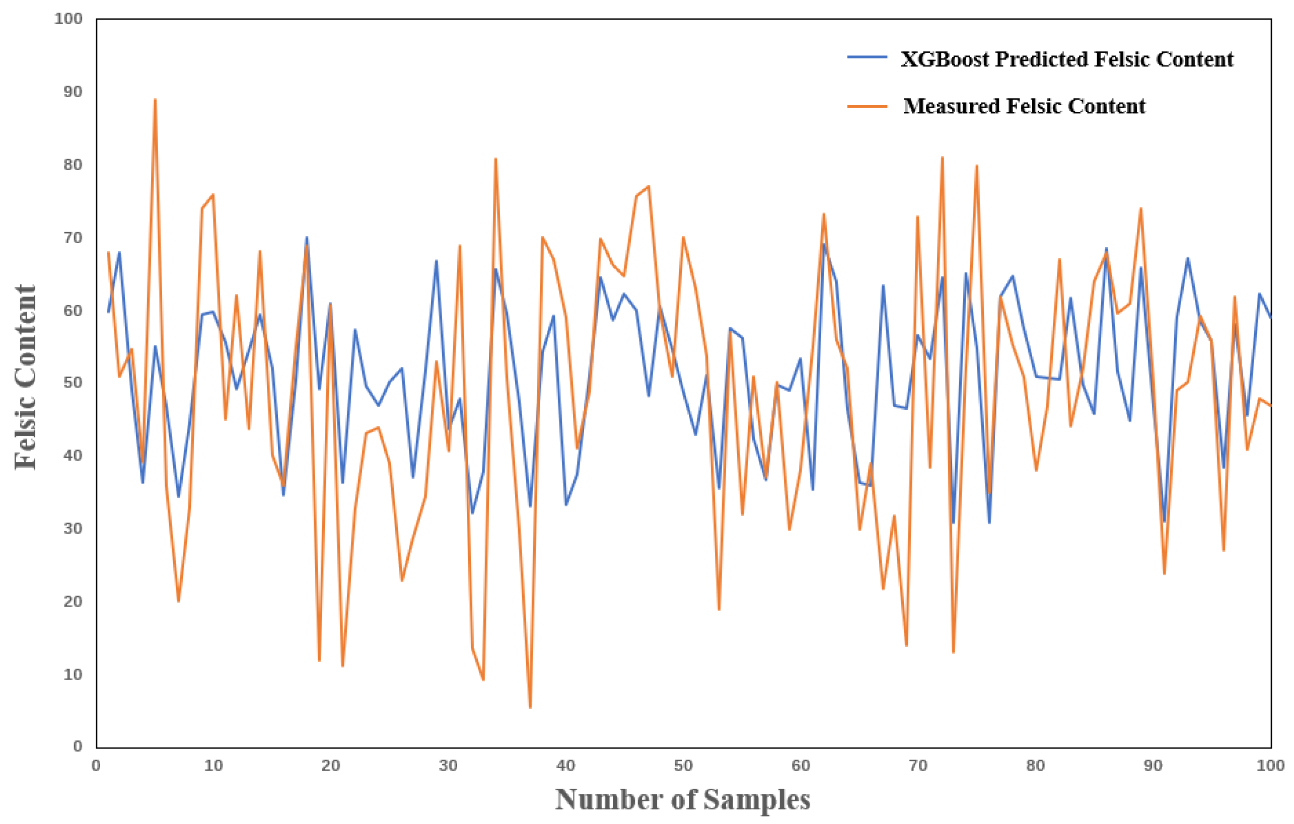
When the proportion of training samples increased to 80% (Table 3), the performance of the XGBoost model was significantly improved: the MAE decreased to 0.12, the MSE slightly dropped to 0.022, and the R² increased to 0.42. This significant improvement indicates that the XGBoost algorithm is relatively sensitive to the training sample size, and increasing the training data can effectively improve its prediction accuracy. It is particularly worth noting that the significant decline in MAE means a reduction in the average absolute gap between the predicted values and the actual values, which is crucial for the precise classification of lithological types, as in this study; the feldspar content is a key indicator for differentiating different lithologies (such as tuff, dolomitic tuff, tuff dolomite, and dolomite). The prediction results are shown in Figure 11.

As shown in Figure 11, the fluctuations of the predicted values are generally similar to those of the actual values. Compared to Figure 10, the number of significant differences between the predicted and actual values at the peaks and troughs has decreased.

3.4.2. SVR Regression Prediction of Felsic Content

Originally, we selected 20% of the predictive factors for training. After achieving the best training results, we input the predictive factors of the test set into the trained model to obtain the predicted results. The evaluation metrics of the predicted results are shown in

Table 4. The SVR model of 20% of the training samples in Well Lu 1 predicting the evaluation index of felsic quality.

	MAE	MSE	RMSE	R2
SVR	0.12	0.021	0.14	0.39

.

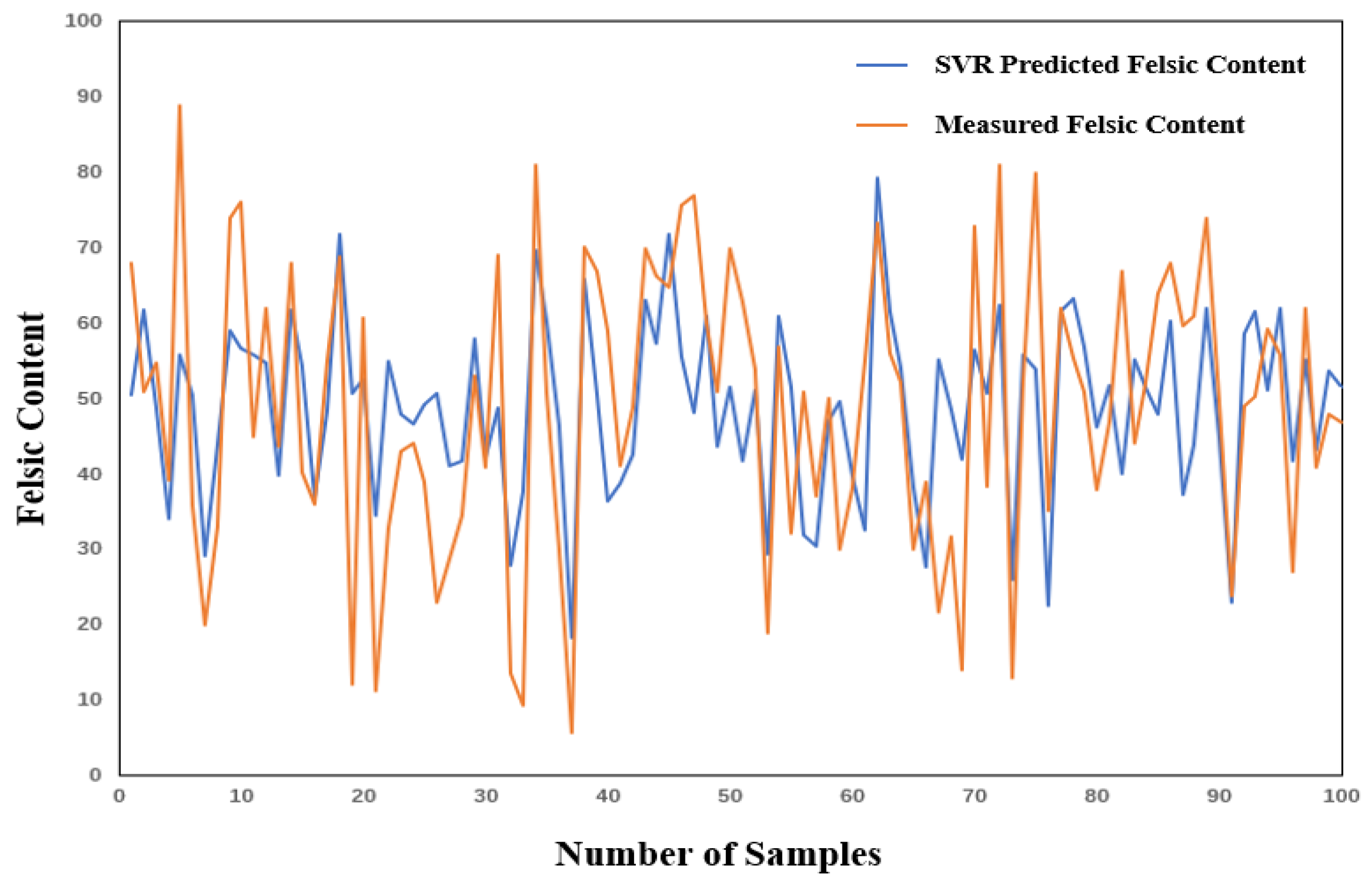
The support vector regression (SVR) model performs well when using 20% of the training samples, as shown in Table 4. Its MAE is 0.12, MSE is 0.021, RMSE is 0.14, and R² is 0.39. Compared with the XGBoost model under the same proportion of training samples, the MAE of SVR decreased by 36.8%, the MSE decreased by 8.7%, and the R² increased by 8.3%. This indicates that under the condition of small samples, the SVR model has a better generalization ability, which may be attributable to its characteristics based on the principle of structural risk minimization, as well as the advantages of the kernel function (the Gaussian kernel used in this study) when dealing with nonlinear relationships.

As shown in Figure 12, the fluctuations of the predicted values by the SVR model are generally similar to those of the actual values, although there are significant differences between the predicted and actual values at some peaks and troughs. Subsequently, 80% of the predictive factors were selected for training. After achieving the best training results, the predictive factors of the test set were input into the trained model to obtain the predicted results. The evaluation metrics of the predicted results are shown in

Table 5. SVR model of 80% of the training samples in Well Lu 1 predicting the evaluation index of the felsic quality.

	MAE	MSE	RMSE	R2
SVR	0.11	0.021	0.14	0.41

.

When the training samples increased to 80% (Table 5), the performance of the SVR model was further improved, with MAE dropping to 0.11 and R² increasing to 0.41. However, compared with the XGBoost model, the performance improvement of the SVR model after increasing the training samples was relatively small (the MAE only decreased by 8.3%, and the R² increased by 5.1%). This phenomenon indicates that the SVR model was able to capture the patterns in the data relatively well under the condition of small samples, and increasing the sample size has a relatively small marginal effect on the improvement of its performance. From the perspective of practical applications, when the available training data is limited, SVR may be a more suitable choice. The prediction results are shown in Figure 13.

3.4.3. Random Forest Prediction of Felsic Content

First, we selected 20% of the predictive factors for training. After achieving the best training results, we input the predictive factors of the test set into the trained model to obtain the predicted results. The evaluation metrics of the predicted results are shown in

Table 6. Random forest model of 20% of the training samples in Well Lu 1 predicting the evaluation index of the felsic quality.

	MAE	MSE	RMSE	R2
Random Forest	0.12	0.022	0.15	0.39

.

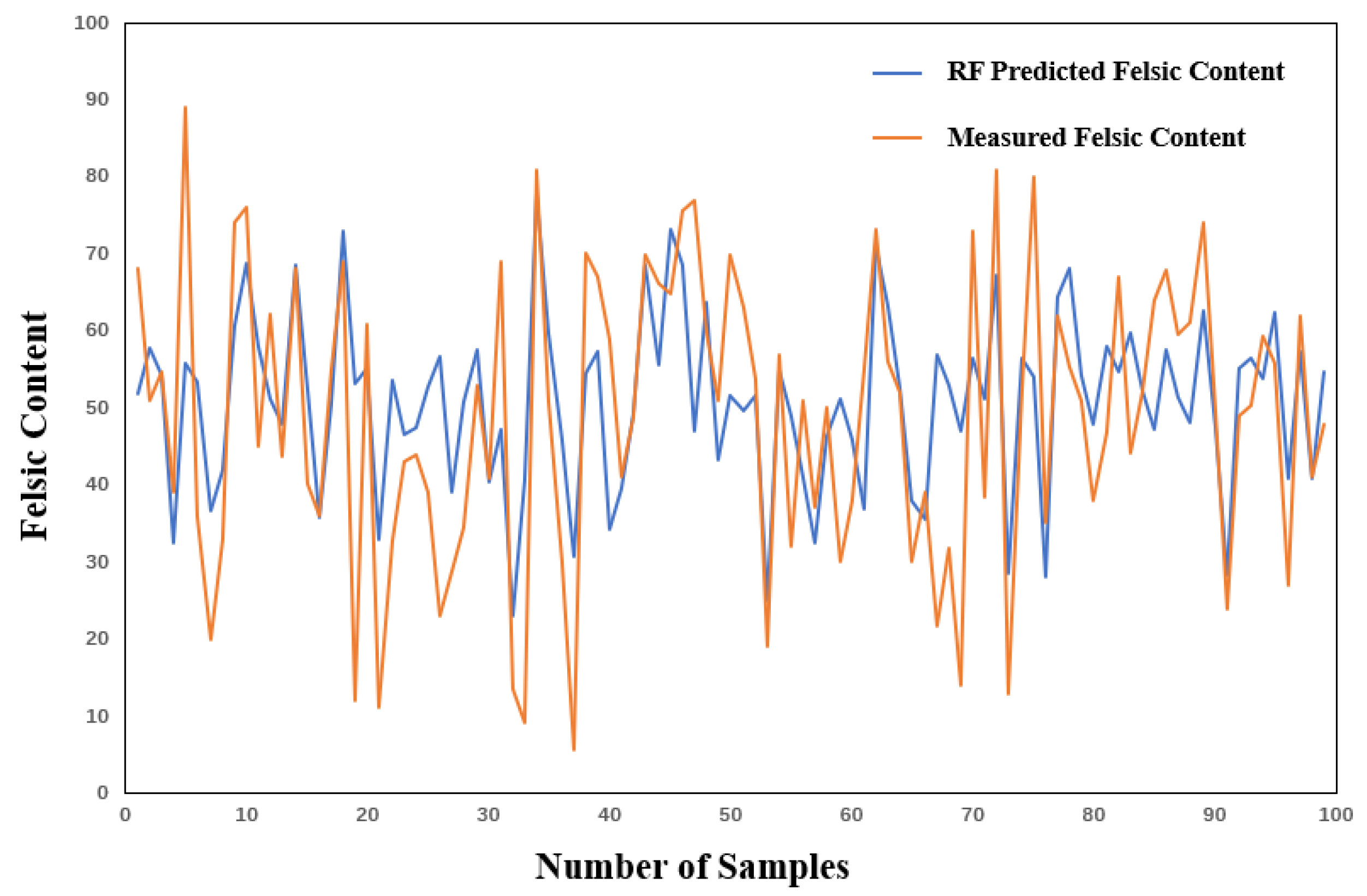
The random forest model performs similarly to SVR under the condition of 20% training samples (Table 6), with an MAE of 0.12, an MSE of 0.022, an RMSE of 0.15, and an R² of 0.39. Although its MSE and RMSE are slightly higher than those of SVR, the MAE and R² of the two are basically the same, indicating that random forest and SVR have similar predictive abilities under the condition of small samples. The prediction results are shown in Figure 14.

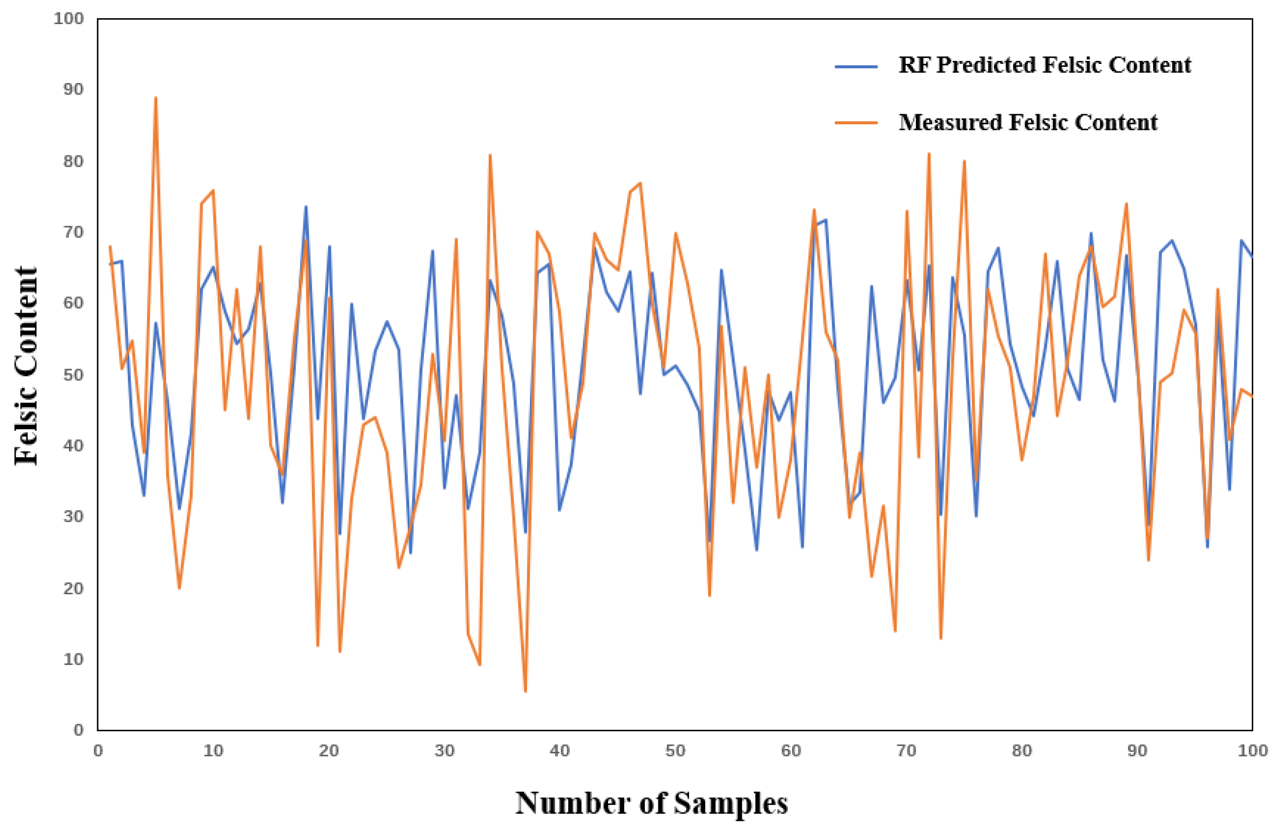
From

Table 7. Random forest model of 80% of the training samples in Well Lu 1 predicting the evaluation index of felsic content.

	MAE	MSE	RMSE	R2
Random Forest	0.11	0.020	0.14	0.43

, it can be seen that the MAE of the random forest model is 0.11, the MSE is 0.020, the RMSE is 0.14, and the R² is 0.43. Compared to the results from training with 20% of the predictive factors, the MAE, MSE, and RMSE from training with 80% of the predictive factors have all slightly decreased, and the R² has slightly improved. The prediction results are shown in Figure 15.

As shown in Figure 15, the fluctuations in the predicted values are generally consistent with those of the actual values. Compared to Figure 14, the alignment of the peaks and troughs has improved.

3.5. Analysis of Example Results

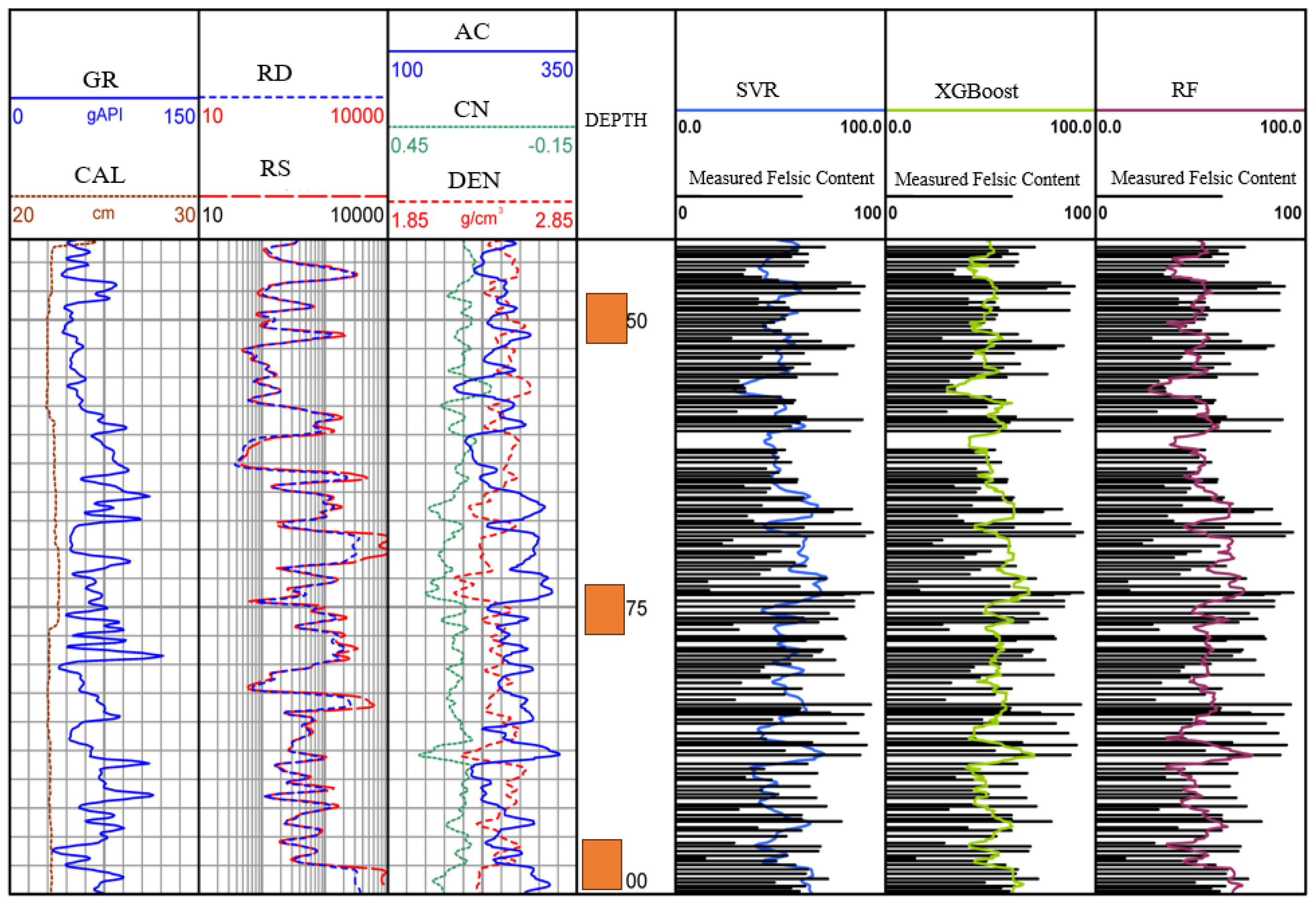
The Lu 1 well was selected for practical applications, and the felsic content of this well was predicted using the three models. Figure 9 shows the prediction results of the three models for the felsic content. It can be seen from Figure 16 that all three models provide good prediction results, with the predicted values generally matching the actual values, and the overall shapes of the predicted curves are similar, with only minor differences in some areas. By comparing the different evaluation metrics of the three methods, it can be concluded that the random forest method provides the most accurate predictions of felsic content.

The analysis shows that the excellent performance of the random forest model mainly stems from the matching of its algorithm design characteristics with the characteristics of the petrophysical data. As an ensemble learning method, random forest effectively alleviates the overfitting problem by aggregating the prediction results of multiple decision trees, which is particularly important for dealing with complex formation characteristic data with a limited sample size. In the identification of complex lithology in the Lucaogou Formation, random forest can capture the nonlinear relationship between logging parameters and long quartz content and has a natural advantage in processing multimodal distributed petrophysical data. In contrast, although support vector regression performs well in finding the optimal hyperplane, it is not as flexible as random forest in dealing with nonlinear relationships.

3.6. Comprehensive Lithology Identification Analysis

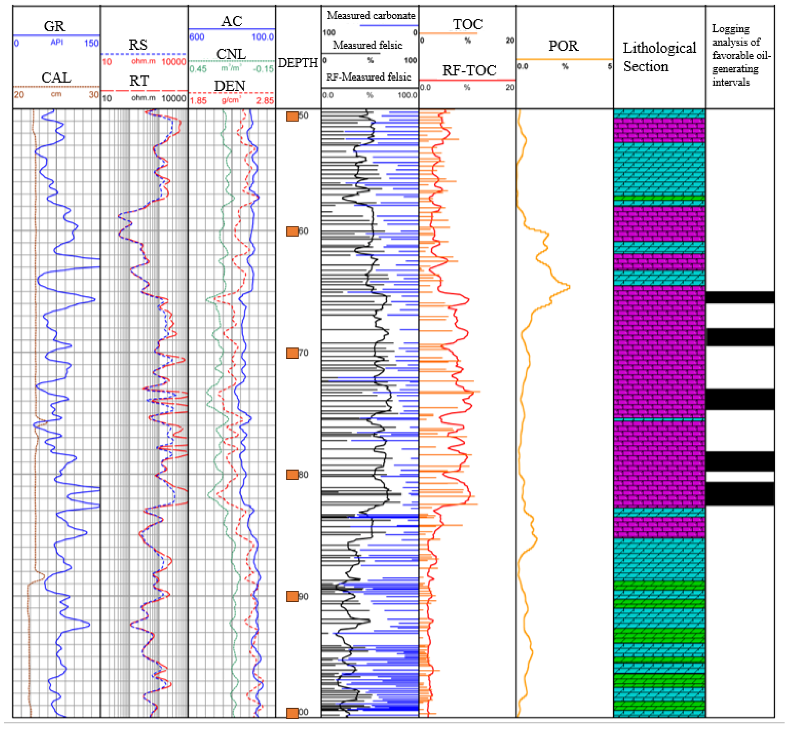
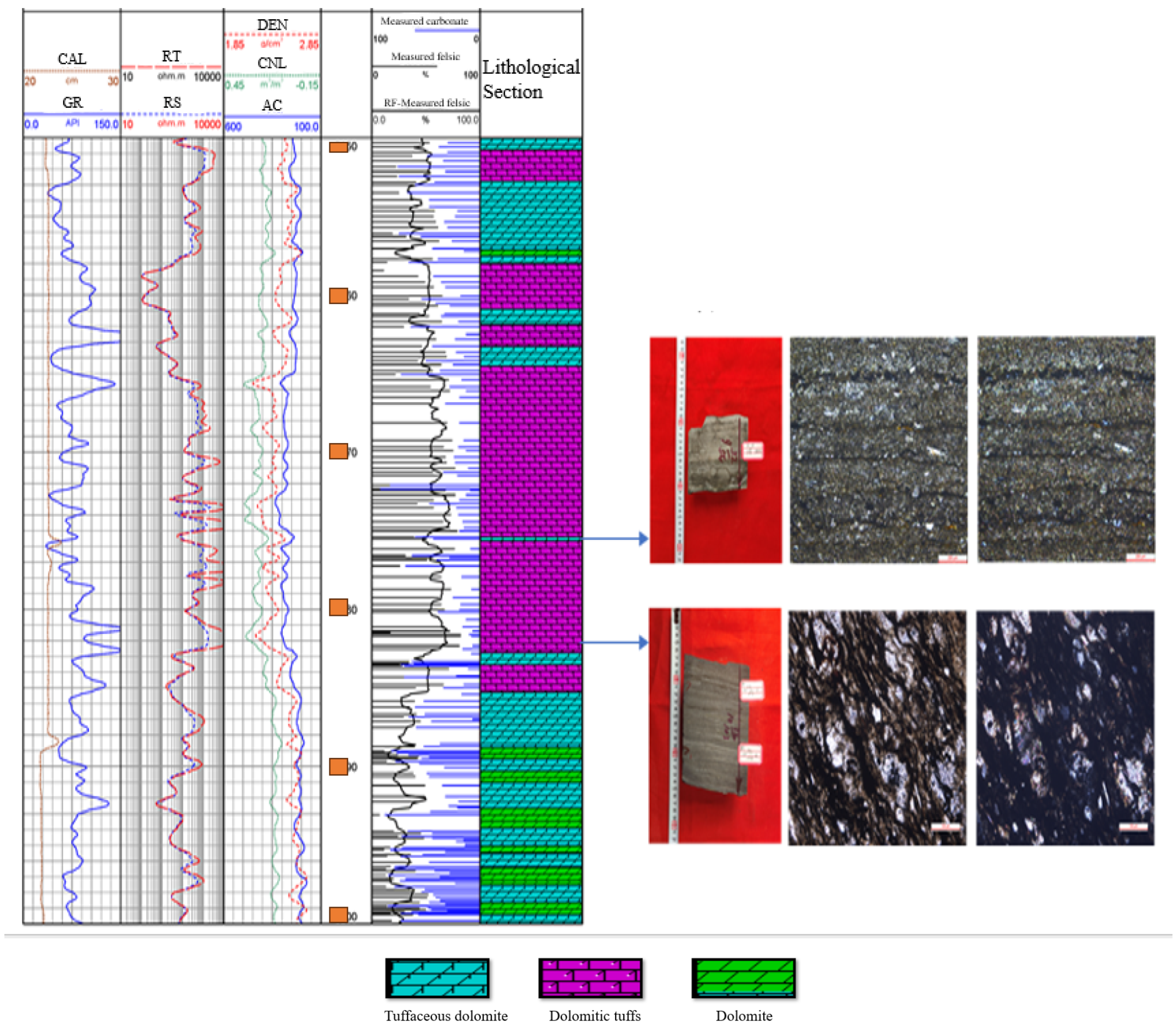
The random forest results, which had the best predictive performance, were selected to identify lithology and favorable reservoirs. The lithology was classified based on felsic content: less than 25% is dolomite, 25–50% is tuffaceous dolomite, 50–75% is dolomitic tuff, and greater than 75% is tuff. Favorable reservoirs were identified based on the TOC content data provided in this paper. The specific results are shown in Figure 17. Combined with the NMR movable fluid porosity curve, it can be concluded that the identification of favorable oil-producing layers is relatively accurate.

As shown in Figure 18, the lithology interpretation log of the Lu 1 well indicates that the XRD-measured felsic content in the core is quite close to the predicted felsic content. This demonstrates that using predicted felsic content for lithology identification yields good results. At a depth of 3175.5 m, the core photograph shows that the lithology is tuffaceous dolomite. According to the XRD data, the main minerals present are felsic minerals and dolomite, with felsic content at 43.1% and dolomite content at 54.7%. The random forest algorithm predicted the felsic content to be 47.14%, which is close to the XRD results. At a depth of 3182.65 m, the core photograph shows that the lithology is dolomitic tuff. According to the XRD data, the main minerals present are felsic minerals and dolomite, with felsic content at 57.1% and dolomite content at 39.2%. The random forest algorithm predicted the felsic content to be 60%, which is also close to the XRD results. By comparing the actual core data with the predicted data, it can be concluded that the prediction results are highly accurate.

According to the XRD analysis, the mineral content is 43.1% felsic and 54.7% dolomite. According to XRD analysis, the mineral content is 57.1% felsic and 39.2% dolomite.

4. Conclusions

This study focuses on the second member of the Lucaogou Formation in the Santanghu Basin, using three machine learning methods to classify and identify lithology in the study area based on conventional logging curves and core data. The specific conclusions of this study are as follows:

• By analyzing the correlations between logging curves, the best feature curves for training were selected. The GR, AC, CN, DEN, RS, and RD curves were chosen as the input features. Three methods—XGBoost, random forest, and support vector regression—were used to predict the felsic content. The predictive performance of the models was evaluated using four evaluation metrics. The random forest method yielded the best performance with R² = 0.43, MAE = 0.11, MSE = 0.020, and RMSE = 0.14 when using 80% of the training data, followed by XGBoost (R² = 0.42, MAE = 0.12, MSE = 0.022, RMSE = 0.15) and then Support Vector Regression (R² = 0.41, MAE = 0.11, MSE = 0.021, RMSE = 0.14). While these R² values indicate moderate predictive capability, they represent a significant improvement over traditional methods in this complex geological setting. By comparing the predicted felsic content with the actual core felsic content at specific depths, it was demonstrated that lithology identification based on predicted felsic content achieves sufficient accuracy for practical reservoir characterization applications.
• In this study, three machine learning methods were adopted to identify the lithology of complex carbonate rocks in the Lujiagou Formation. Compared with previous studies, our random forest model has achieved better results in the prediction of feldspar content by optimizing feature selection. Although the R² value of the model is at a medium level, it is comparable to the previous achievements under similar complex geological conditions and achieves a good balance between computational efficiency and accuracy. Verified by actual core data, the lithology identification method based on predicted feldspar content has practical value, providing a reliable technical solution for complex lithology identification and having reference significance for reservoir evaluation in similar areas.
• Although the prediction model constructed in this study performed well in the lithology identification of the Lucaogou Formation, there are still some limitations and uncertainties: On the one hand, the logging data itself contains various noise sources and uncertainties. Although certain data preprocessing has been carried out, some noises may still affect the prediction accuracy. On the other hand, the number of XRD samples available for model training in this study is limited, which may affect the model’s ability to fully capture the geological complexity of the region. Secondly, there is a potential sampling deviation. Some core samples may not perfectly represent all the lithological changes existing in the formation. To alleviate these uncertainties, future work should focus on expanding the training dataset, adding additional logging curves when available, and developing more complex model validation techniques.
• Although this research has achieved certain results, there is still room for improvement. Future research can be carried out from the following perspectives: Firstly, on the basis of sufficient data, deep learning methods such as convolutional neural networks (CNNs) and recurrent neural networks (RNNs) can be used to predict complex rock types. Deep learning methods have good effects in capturing the tiny changes between different rock types. Secondly, other data types such as nuclear magnetic resonance (NMR) can be combined to enhance the lithology discrimination ability of the model in the case of overlapping conventional logging responses.