1. Introduction
Radar systems on maritime aircrafts, especially those used for anti-ship missiles, frequently encounter significant detection challenges when the target is close to marine geographical features (MGFs) such as islands and offshore drilling platforms with pronounced electromagnetic characteristics. The challenges arise primarily from two aspects:
(1) The detection blind zones caused by MGFs. MGFs can create physical obstructions that block the radar beam, resulting in areas where the radar cannot detect targets. This is particularly problematic for sea-skimming aircraft when the target is located behind MGFs.
(2) The radar target adhesion (RTA) problem caused by MGFs. Even when the target is within the radar line of sight (LOS), the limitations in radar resolution and the electromagnetic interference from MGFs may also lead to the RTA problem. In this case, the target can be mistakenly merged with MGFs and identified as a single target [
1].
To address these challenges, current technical research primarily focuses on ensuring that target signals can be detected by radar as well as avoiding the RTA problem. Efforts include improving radar resolution and imaging capabilities [
2,
3] and developing relevant algorithms [
4,
5,
6,
7,
8,
9,
10,
11,
12,
13,
14]. While these research directions are theoretically significant, there are still several technical barriers and hardware limitations for their practical application.
From a tactical perspective, optimizing aircraft operations is crucial for overcoming these challenges. This can be achieved by selecting appropriate radar activation points and flight directions to improve the ability of radar correctly identifying the target, even with limited radar resolution and LOS conditions. In this context, several studies have made notable contributions: Hou, Chen, and Dong [
15,
16,
17] simplified MGFs and targets into point mass models, providing a theoretical basis for evaluating target identification conditions based on radar range and azimuth angle resolution. However, this method can introduce significant errors, especially for complex MGFs like large islands. To address these limitations, based on the 2D contour data of MGFs, Wang [
18] attempted to enhance radar’s ability to distinguish targets from MGFs by adjusting the aircraft’s search direction, and Xie [
19] assessed the number of “false targets” that coastlines may generate in a radar system with radar azimuth angle resolution; Wu [
20] proposed a strategy to optimize the aircraft’s searching direction, ensuring the radar search range covers the target while avoiding MGFs using radar range resolution. Despite these efforts, existing methods still have notable limitations:
(1) They do not account for the influence of MGFs’ elevation data and radar elevation angle resolution, limiting their applicability to sea-skimming aircraft and making them unsuitable for advanced high-altitude aircraft;
(2) They ignore potential errors, such as radar activation point errors and MGF position errors. So, they can only provide a binary result of “identified” or “unidentified” and cannot quantitatively calculate the probability of the target being correctly identified by radar at a specific marine location.
With the developments in equipment technology, the usage of advanced high-altitude aircraft is increasing due to their broader field of view, faster speed, and longer range. As for the radar LOS and RTA problems with analysis of high-altitude aircraft in 3D space, it is essential to incorporate the 3D model of MGFs, radar elevation angle resolution, and related errors. Therefore, this paper proposes a method to calculate the radar identification probability (Pident) for a target at a specific marine location. Compared to the existing methods, the proposed method has advantages as follows:
(1) The proposed method further considers the influence of MGFs’ elevation data and radar elevation angle resolution, so that it can be applied to aircraft at any altitude, better aligning with the advanced aircraft’s performance and requirements.
(2) The proposed method integrates errors from both the MGFs and the aircraft and employs the Monte Carlo method to obtain Pident, instead of the binary result from the existing method, providing more accurate and intuitive decision-making support for the mission planning of maritime aircraft.
2. Principle of Radar Identification Probability Calculation
2.1. Criteria for Radar Identification in 3D Space
As previously discussed, the challenges of radar identification caused by MGFs stem from two main aspects: radar detection blind zones and the RTA problem. To address the former, it is essential to ensure that the target is within the radar LOS. In terms of the RTA problem, it primarily depends on the radar resolution.
Radar resolution can be categorized into range and angular resolutions in the spatial domain. Range resolution refers to the minimum distance between two adjacent targets that the radar can distinguish, primarily determined by the radar signal’s bandwidth and pulse width. Angular resolution can be further divided into azimuth angle resolution and elevation angle resolution, which refer to the minimum angles for radar to distinguish two adjacent targets in horizontal and vertical directions, respectively. These are mainly dependent on the radar antenna’s beamwidth.
Existing methods [
15,
16,
17,
18,
19,
20] have mostly simplified MGFs to point masses or relied solely on their 2D contour data, focusing mainly on radar range and azimuth angle resolution within a 2D plane. However, these methods did not fully consider the influence of elevation angle resolution. To extend the research scope from 2D to 3D for advanced high-altitude aircraft, this paper introduces radar elevation angle resolution and an MGF 3D model.
When considering only the spatial domain and ignoring factors such as Doppler resolution, the RTA problem occurs when two or more objects are within the radar LOS and their differences in range, azimuth angle, and elevation angle relative to the radar are all smaller than the respective resolutions.
To more precisely quantify and describe the criteria for the RTA problem in 3D space, this paper establishes a local Cartesian coordinate system with the due north direction as the
X-axis, the due east direction as the
Y-axis, the instantaneous sea surface as the
XOY plane, and the
Z-axis pointing vertically upward. Two targets are denoted as the points
T1(
XT1,
YT1,
ZT1) and
T2(
XT2,
YT2,
ZT2), and the radar position is denoted as the point
S(
XS,
YS,
ZS). The schematic diagram of the relative positional relationship between these points is shown in
Figure 1.
In
Figure 1,
dST1 and
dST2,
AST1 and
AST2, and
EST1 and
EST2 represent the distances, azimuth angles and elevation angles from point
S to points
T1 and
T2, respectively. According to the definition of RTA, given the radar range resolution
Rres, azimuth angle resolution
Ares, and elevation angle resolution
Eres, when both
T1 and
T2 are within the radar LOS, the condition for the radar to misidentify
T1 and
T2 as a single target is that Equations (1)–(3) are simultaneously satisfied.
The terms in Equations (1)–(3) are as follows:
Therefore, in this paper, the conditions for a target to be correctly identified by the radar are:
(1) The target is within the radar LOS;
(2) If there are any interfering objects within the radar LOS in addition to the target, Equations (1)–(3) are not simultaneously satisfied.
After establishing the radar identification criteria in 3D space, the potential errors from both the MGF and the maritime aircraft are further analyzed in the following section.
2.2. Error Analysis
In addition to the limitations of radar LOS and resolution, potential errors can also affect radar identification. This paper focuses on errors from two sources: the MGF and the maritime radar (aircraft). For MGF data, the errors are mainly due to the accuracy of geospatial surveys. There are planar position errors (Δ
XB, Δ
YB) and elevation data error Δ
ZB. (Δ
XB, Δ
YB) are assumed to follow a 2D normal distribution with independent directions, an expected value of 0, and a standard deviation of
σBXY for both directions. Δ
ZB is assumed to follow a normal distribution with an expected value of 0 and a standard deviation of
σBZ:
The errors from the radar (aircraft) mainly stem from the radar system’s hardware precision and the navigation errors of the aircraft and its launch platform. They primarily consist of three aspects: the planar position error of the aircraft launch platform (Δ
XL, Δ
YL), the planar position error (Δ
XS, Δ
YS), and the elevation error Δ
ZS of the radar activation point. Similarly, these errors are assumed to follow the normal distributions:
To simplify the calculations, this paper combines (Δ
XS, Δ
YS), (Δ
XL, Δ
YL), and (Δ
XB, Δ
YB) as shown in Equation (10), so that (Δ
XS, Δ
YS) can be equivalently considered to follow the 2D normal distribution as shown in Equation (11):
Similarly, Δ
ZB and Δ
ZS are combined as follows:
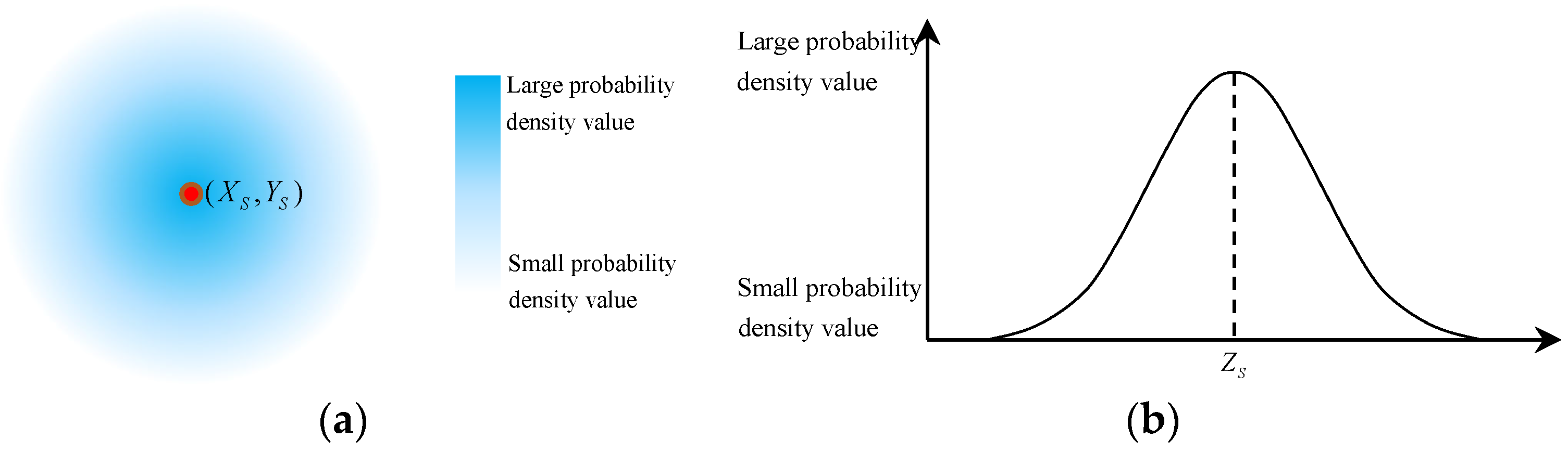
In summary, the errors from both the MGF and the radar (aircraft) are combined and equivalently regarded as the errors of
S, whose planar error (Δ
XS, Δ
YS) and elevation error Δ
ZS follow the normal distributions shown in Equations (11) and (13), respectively. Based on that, the actual radar activation point with errors
S′(
XS′,
YS′,
ZS′) and its distribution are shown in Equations (14)–(16), and the schematic diagram of that is shown in
Figure 2.
In Equations (14)–(16) and
Figure 2,
S(
XS,
YS,
ZS) is the theoretical radar activation point.
With the error analysis completed, the detailed steps for calculating the radar identification probability using the Monte Carlo method would be presented.
2.3. Calculation Steps
In this paper, the actual radar operation process is simplified since we paid more attention to the impact of the limitations of radar resolutions and electromagnetic interference from MGFs, and the relevant assumptions are as follows:
Assumption 1. All objects mentioned in this paper are within the theoretical searching range of the radar.
Assumption 2. If the line connecting radar and target is occluded by an MGF, the target would be out of radar LOS and cannot be detected or identified.
Assumption 3. If there is no LOS limitation or RTA problem, the target would be correctly identified by the radar, regardless of the dynamic environmental factors, such as sea state or weather.
Assumption 4. The result probability Pident only corresponds to the moment when the radar is activated at point S.
Based on these assumptions, the process of calculating the probability
Pident is shown in
Figure 3.
In
Figure 3, the specific implementation process of each step is as follows:
Step 1: Input Data. Based on the 3D model of MGFs, extract the points with pronounced electromagnetic characteristics, denoted as Bi(XBi, YBi, ZBi) (i = 1,2, …, N), and input their planar position and elevation error standard deviation σBXY and σBZ. According to the aircraft’s mission planning and performance parameters, input the radar activation point S(XS, YS, ZS) and its planar position and elevation error standard deviation σSXY and σSZ (for sea-skimming aircraft, ZS and σSZ can be set as 0), aircraft launch platform planar position error standard deviation σL, radar range resolution Rres, elevation angle resolution Eres, and azimuth angle resolution Ares. Finally, input the marine location point T(XT,YT) where Pident is to be calculated.
Step 2: Monte Carlo Simulation. Set the Monte Carlo repetition times Mrepeat and initialize the counter Mident = 0. In each simulation:
(1) Randomly generate the radar position point S′(XS′, YS′, ZS′) based on the theoretical values and errors from Step 1 using Equations (5)–(16).
(2) Determine whether T is within the LOS of S′. If it is, proceed to the next step; otherwise, proceed to the next simulation.
(3) Sequentially determine whether S′, T, and each Bi simultaneously satisfy Equations (1)–(3). If none of them satisfies the condition, increment Mident by 1; otherwise, proceed to the next simulation.
Repeat the simulation Mrepeat times.
Step 3: Calculate
Pident. Calculate the ratio of
Mident to
Mrepeat to obtain
Pident, as shown in Equation (17):
Due to the instability of the Monte Carlo method, the accuracy of Pident can be improved by increasing Mrepeat in Step 2.
By inputting the marine location points around the MGF and repeating the above steps, the distribution of Pident around the MGF can be visually expressed.
3. Simulation and Analysis
3.1. Data Input
To validate the effectiveness and applicability of the proposed method across different scenarios, a series of simulation experiments were conducted. According to the calculation process of
Pident shown in
Figure 3, the experiment first required the input of data.
To simplify the simulation, it was assumed that all points of the MGF possess pronounced electromagnetic characteristics. Based on this assumption, the experiment used points read from the MGF’s stl file as the
Bi(
XBi,
YBi,
ZBi) (
i = 1,2, …,
N) for data input. The stl format is a file format that describes the surface geometry of a 3D object with multiple triangular facets. Its binary format is shown in
Table 1.
Since the triangular facets of the MGF were obtained using the file format in
Table 1, it was accessible to determine whether the marine location point was within the radar LOS by checking whether the line connecting the radar position point and the marine location point intersected with any of the triangular facets. The
Bi(
XBi,
YBi,
ZBi) (
i = 1, 2, …,
N) data could be used to determine whether the RTA problem occurred.
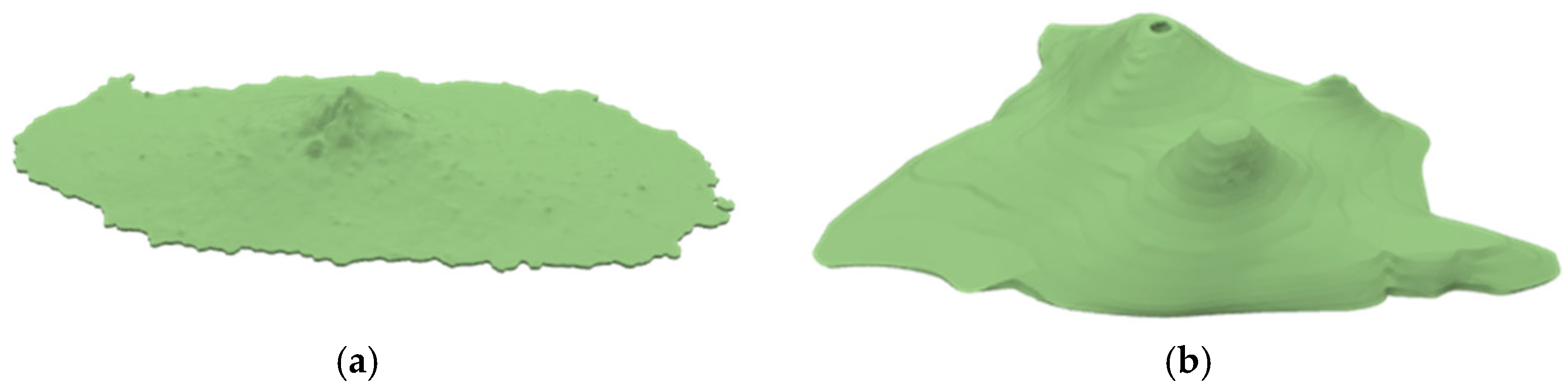
Based on that, two islands of different shapes were used as the MGFs for the experiment. The 3D models and parameters of the MGFs are shown in
Figure 4 and
Table 2.
Since the planar geometric center of the experimental MGFs are close to the coordinate origin, for the convenience of subsequent calculations and explanations, the distance, azimuth angle, and elevation angle between the radar and the coordinate origin are considered as those between the radar and the MGFs for the experiment.
In addition to the MGF, the experiment simulated reasonable types of virtual maritime aircraft and the onboard radar. The specific parameters of them and other parameters for the simulation are shown in
Table 3.
To verify the applicability of the proposed method to aircraft at any altitude, three groups of radar position points were constructed, as shown in
Table 4.
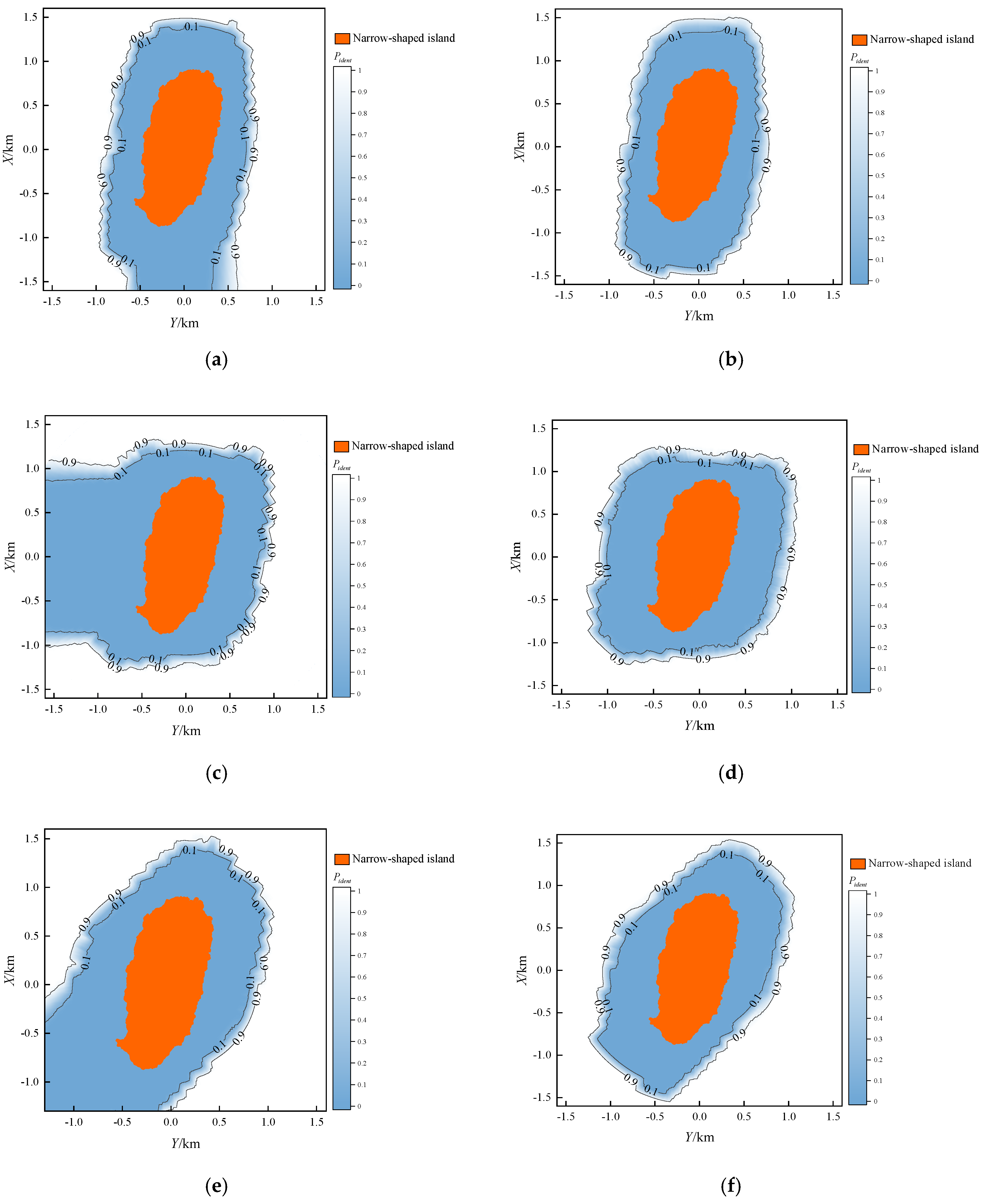
3.2. Result Calculation
With
Mrepeat set to 10,000 and the input data from
Section 3.1, we calculated and visualized the
Pident distribution around the MGFs for the experiment under the radar points from
S1 to
S6. The results are shown in
Figure 5 and
Figure 6.
3.3. Result Analysis
For ease of description, in this paper, the marine areas around the MGF for the experiment were denoted as different levels according to their value of
Pident as shown in
Table 5.
As illustrated in
Figure 5 and
Figure 6, the proposed method effectively calculates and visualizes the
Pident distribution around the MGFs for both sea-skimming and high-altitude scenarios.
Combining
Figure 5 and
Figure 6 and
Table 4, it can be observed that, the Level I and II regions always mirror the MGF’s outline but are stretched along the radar’s azimuth bearing. For example, when the radar is north of MGFs (0° azimuth) in
Figure 5b and
Figure 6b, the Level I and II regions extend along the
X-axis as “enlarged copies” of both narrow-shaped island and triangular-shaped island; when radar moves east (90° azimuth) in
Figure 5d and
Figure 6d, they lengthen along the
Y-axis. These are consistent with physical expectations and provide an initial validation of the proposed method.
Furthermore, Given the same distance and azimuth angle between the MGF and the radar, the changes in elevation angle caused by the decrease in ZS (from high-altitude to sea-skimming) also result in the shapes of the Level I and Level II regions extending towards the azimuth direction of the aircraft. This indicates that the threat level of the marine areas around the MGF is enhanced, consistent with the radar detection blind zones caused by MGF occlusion for sea-skimming aircraft, further demonstrating the effectiveness of the proposed method in this paper.
In addition to the overall result, we selected marine location points
Ta (0.6 km, −0.8 km) for the narrow-shaped island and
Tb (0.6 km, −0.6 km) for the triangular-shaped island as individual cases since they were always within the LOS of radar at the point of S
1, S
2, S
5, and S
6. The corresponding probabilities were extracted and shown in
Table 6.
From
Table 6, it can be seen that, even for
Ta and
Tb which always satisfied the radar LOS condition, changes in the aircraft state still have a significant impact on
Pident. For
S5 and
S6, under the interference of the narrow-shaped island, the change in aircraft state from sea-skimming to high-altitude increased the
Pident of
Ta by 0.5010; for
S1 and
S2, under the interference of the triangular-shaped island, the change in aircraft state from sea-skimming to high-altitude increased the
Pident of
Tb by 0.3328. This indicates the importance of introducing the radar elevation angle resolution and MGF 3D model, and the necessity of the proposed method.
3.4. Practical Application
In actual application scenarios, the complex relationship between radar activation point, MGF data, and Pident is further compounded by dynamic maritime environment, aircraft performance, and specific mission requirement. Owing to the non-linear interaction among these factors, analytically determining the single optimal radar activation point, either by maximizing Pident at a given target location or by minimizing the combined extent of Level I and Level II regions, is computationally intractable and often operationally impractical.
The proposed method circumvents this difficulty by providing planners with an explicit, probability-based comparison of candidate configurations. The Inputs consist of
(1) The 3D MGF model;
(2) The area around the MGF whose Pident needs be calculated;
(3) Radar resolution parameters;
(5) A discrete set of candidate radar activation points that satisfy the constraints.
The proposed method would then return the corresponding Pident values, and the mission planners can select the most operationally suitable radar activation point from candidates without recourse to exhaustive numerical optimization.
Example. Consider the narrow-shaped island scenario with two candidate radar activation points S2 and S6 due to the constraints. If surveillance intelligence indicates that a target is expected at location Ta, and the computed probabilities are Pident(S2) = 0.9990 and Pident(S6) = 0.5887. The planner therefore selects S2, achieving a substantial increase in identification confidence.
3.5. Result Comparison
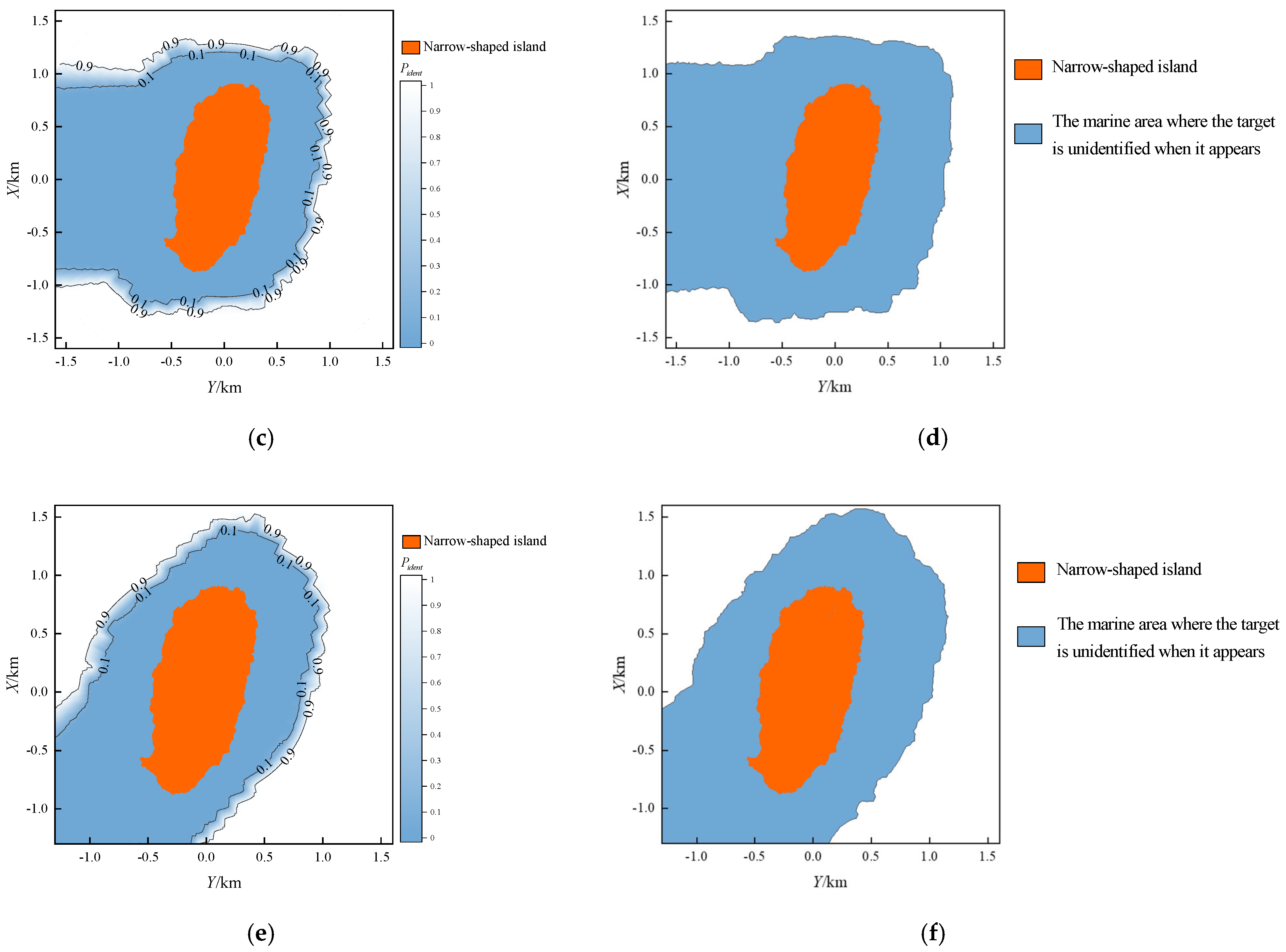
To compare the results from the proposed method and existing methods, we first need to clarify the calculation principle of the existing methods. Existing methods predominantly utilize the 2D contour data of MGFs and are limited to sea-skimming aircraft. These methods do not account for potential errors and merely provide a binary result of “identified” or “unidentified” rather than a probability of identification. The relevant calculation is based on the 2D contour data of MGFs, using the LOS condition and Equations (1) and (2), while neglecting the impact of radar elevation angle resolution (Equation (3)). As these methods do not incorporate error considerations, there is no requirement for Monte Carlo simulation.
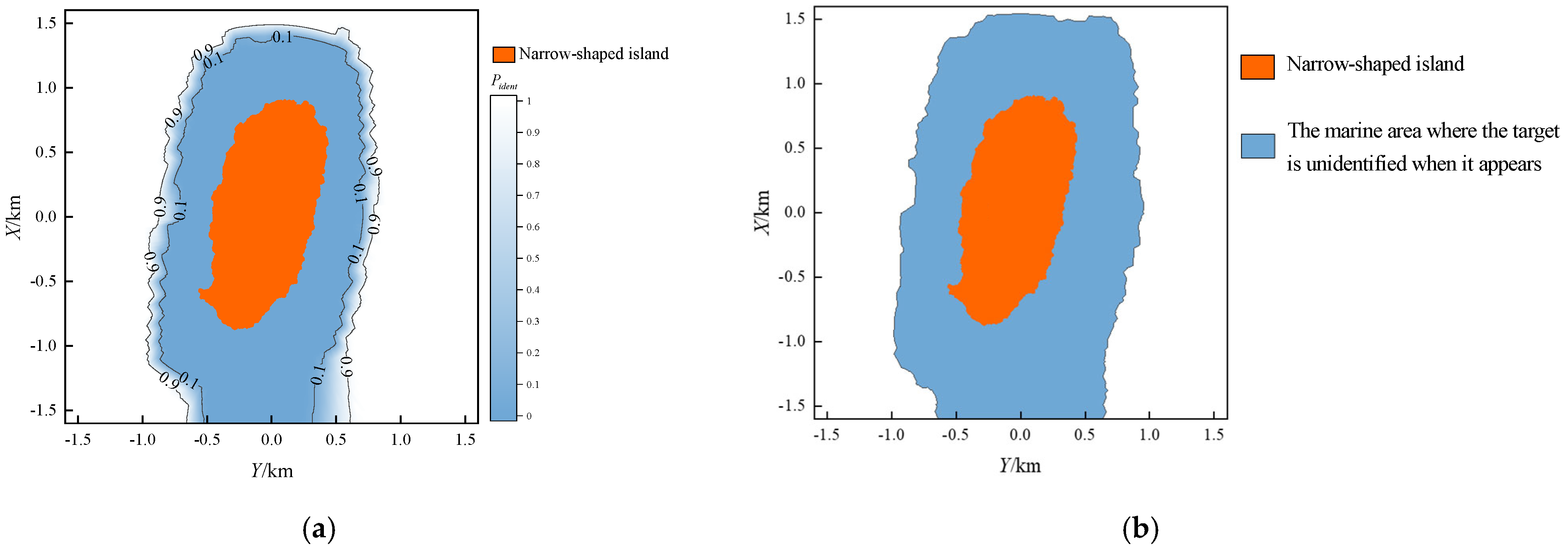
To further illustrate the differences between the proposed method and existing methods, we selected radar position points
S1,
S3, and
S5 as examples (sea-skimming aircraft), and calculated and visualized the binary result surrounding the narrow-shaped island. The comparison of these results with those obtained from the proposed method is shown in
Figure 7.
From
Figure 7, it can be seen that the shape and area of the “unidentified” region from existing methods is similar to those of the sum of Level I and Level II regions from the proposed method, which validates the effectiveness of the proposed method from a different angle.
Besides that, the proposed method not only can be applied to aircraft at any altitude, but it can also take more errors into consideration, and the probability result rather than the binary result provides more precise and intuitive decision-making support for aircraft mission planners.
The detailed comparison between the proposed method and the existing methods in terms of RTA determination conditions, MGF data utilization, and other factors is shown in
Table 7.
In summary, the proposed method, which incorporates radar elevation angle resolution and the MGF 3D model, is applicable to aircraft at any altitude in 3D space. It can quantitatively calculate the probability of radar correctly identifying a target at a specific marine location, providing more precise and intuitive decision-making support for aircraft mission planners. Compared with existing methods, it better aligns with the current performance and requirements of aircraft.
4. Conclusions
Based on theoretical derivation and simulation analysis, the conclusions are as follows:
(1) In contrast to existing methods limited to sea-skimming aircraft, the proposed method offers a significant advancement by being applicable to aircraft at any altitude.
(2) With the input parameters, the proposed method can effectively calculate the probability Pident of the target closed to MGF being correctly identified by the radar, rather than a binary result of “identified” or “unidentified” from existing methods, which helps provide more precise and intuitive decision-making support for aircraft mission planners.
However, we acknowledge that our current model does not account for dynamic environmental factors such as sea state or weather conditions, nor does it consider the correlations between the mentioned errors. Future work will focus on incorporating these elements to enhance model accuracy and robustness. Specifically, we plan to analyze error correlations to refine our method, which means that the distribution for actual radar activation point S′(XS′, YS′, ZS′) would consider the covariances between MGFs and aircraft caused by dynamic environmental factors, and each Monte Carlo simulation would then sample from this refined distribution, yielding more accurate and robust probability results.


