Galerkin’s Spectral Method in the Analysis of Antenna Wall Operation

Abstract

In this paper, a solution to the problem of electromagnetic field scattering on a periodic, constrained, planar antenna structure placed on the boundary of two dielectric media was formulated. The scattering matrix of such a structure was derived, and its generalization for the case of an antenna with a multilayer dielectric substrate was defined. By applying the Galerkin spectral method, the problem was reduced to a system of algebraic equations for the coefficients of current distribution on metal elements of the antenna grid, considering the distribution of the electromagnetic field on Floquet harmonics. The finite transverse dimension of the antenna was considered by introducing, to the solution of the case of an unconstrained antenna, a window function on the antenna aperture. The presented formalism allows modeling the operation of periodic, dielectric, composite antenna arrays.

1. Introduction

Printed antennas have been some of the most innovative areas of antenna technology for a dozen or so years. In the early fifties, radiation from strip and microstrip lines was observed. From the point of view of the use of transmission lines, however, this was an undesirable phenomenon; so, apart from a few articles suggesting its use in the construction of antennas, it did not arouse much interest. Until 1971, most published works were only in the form of presentations of experimental results. It was not until the seventies that rapid development in theoretical and experimental work on this type of antenna began. In 1979, the first international conference was held in La Cruses, devoted to a comprehensive approach to antennas on a dielectric substrate, i.e., materials, construction plans, configuration systems and theoretical foundations. Microstrip antennas are characterized by many interesting features, such as the following:

• Precise mapping on the surface;
• Low manufacturing cost;
• High repeatability of execution;
• Small volume;
• Masking of the operating frequency;
• Simplicity of manufacturing provided that relatively advanced technologies are used;
• Flat shape and low weight, which allow the use of antennas on a dielectric substrate on fast flying objects without the risk of deterioration of their aerodynamic properties.

These antennas allow for miniaturization of the antenna system and thus its greater density. This causes mutual couplings to occur, changing the field distributions on aperture antennas and the current distributions in linear antennas. This situation in turn changes the spatial radiation characteristics of the antennas and their impedance inputs.

The spectral response of an antenna array placed in a homogeneous dielectric medium depends on the antenna geometry, medium parameters, angle of incidence, polarization and geometry of the exciting field. However, in many applications, the above number of parameters determining the operation of the antenna is not sufficient to model its desired directional characteristics. An increase in the number of parameters of the antenna structure can be obtained by introducing a multilayer dielectric medium with a specified number of metalized periodic surfaces placed on flat boundaries between dielectric layers [1,2,3,4,5,6,7,8,9,10,11,12,13]. There are two complementary approaches to the analysis of such structures. In the first, the composite antenna system is analyzed by constructing supermodes of the entire structure; in the second, the system is considered as a cascaded composition of planar discrete elements, i.e., boundaries between two dielectrics, periodic metallized planes and dielectric layers. The latter approach leads to the definition of the scattering, transmission or impedance matrix of the entire structure by cascaded composition of appropriate matrices assigned to individual discrete elements of the antenna structure. It is particularly useful in modeling dielectric multilayer antenna walls, where the stored data concerning one planar antenna element can be repeatedly used in the analysis of different antenna systems with modified parameters of the remaining discrete elements of the structure. In practice, antenna arrays are most often composed of periodic metal structures placed on or immersed in a dielectric multilayer medium. Changes in the size and shape of individual antenna elements enable effective modeling of their spectral characteristics; these changes can be additionally modeled by selecting the geometrical and physical parameters of the dielectric layered substrate and coating [1,2,3,4,5,6,7,8,9,10,11,12,13]. In the case of large transverse dimensions of the antenna of the order of 100 wavelengths and several dozen or more individual metal radiation elements, the radiation properties of the antenna correspond to the properties of an unconstrained antenna structure to a good approximation. When the condition of periodicity of such an antenna and its excitation with linear, uniform phase modulation is met, the problem of scattering on such a structure is reduced to the analysis of one basic antenna cell, usually in the spectral space spanned by a complete system of corresponding Floquet harmonics [13,14,15]. Nevertheless, for antenna arrays composed of a dozen or so basic cells of regular shapes, this method gives good results. Other known methods of solving the scattering problem on larger periodic structures, such as modifications of the above-mentioned direct method by limiting the number of basic functions and appropriately selecting their courses [16,17,18] or the iterative method imposed on the solution by successive application of the fast Fourier transform, are approximate, slowly convergent and can be used only in certain simple cases convenient for analysis.

The analysis presented in this paper is based on the concept of the window function [6,10,19,20,21,22,23,24] imposed on the sought current distribution and incorporated into the structure of the radiation problem of a periodic unconstrained structure. The generalized spectral analysis, for an unconstrained one, is, after some adaptations, particularly convenient for carrying out the concept of adaptation of the window function due to the full system of Floquet harmonics used in solving the problem. The sequence of successive solution steps presented in the paper should lead to an exact solution, considering the anticipated difficulties with convergence of the applied procedure.

In Section 2, the factorization of the scattered field in the spectral space is derived in an exact manner, specifying the grid coefficient function and indicating the possibility of its use in the approximate analysis of the scattering problem on a limited antenna structure. Section 3 [25,26] contains careful specification of the solution of the scattering problem on an unconstrained structure in terms of direct application of this formalism to the case of an antenna of limited dimensions. The procedure for adapting this formalism is presented in Section 4 [27], with the necessary modifications introduced by an appropriately defined window function. The accuracy of the solution method is verified by the proposed iterative procedure using a system of algebraic equations for the spectral coefficients of the distribution of field quantities and currents. In this paper, the use of window functions is proposed, and the full Floquet harmonic system is also used to solve the problem. A sequence of subsequent solution steps is also proposed to lead to a strictly numerically convergent solution.

2. Radiation Field of Unconfined Antenna Array Placed on Multilayer Dielectric

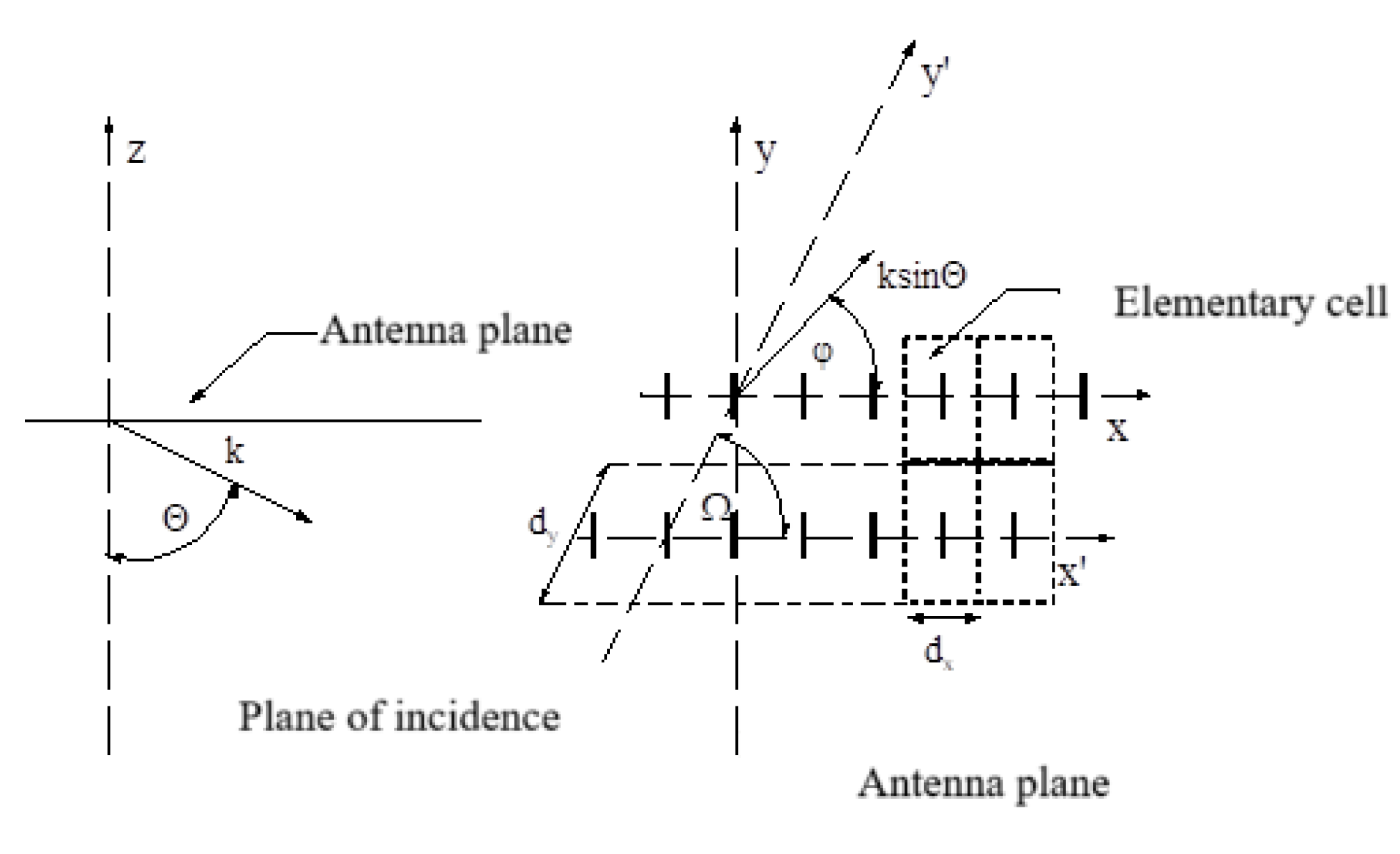
The geometry of the analyzed antenna array and the adopted coordinate system are shown in Figure 1. It shows an antenna located in free space, and the case of the antenna location on the boundary of two different dielectric media is specified only by the form of Green’s function. In this work, the special case of a rectangular antenna grid is considered, i.e., Ω = π⁄2, although generalization of the analysis to the case of a skew antenna grid Ω ≠ π⁄2 does not change the presented procedure for solving the scattering problem.

The relationship between the scattered fields in the observation plane (x,y,z)

$${\underset{\_}{E}}_t^s(x,y,z)={\int }_{-\infty }^{+\infty }{\int }_{-\infty }^{+\infty }\underset{\_}{F}\left({\underset{\_}{E}}_t^s\right)(k_x,k_y,z)\mathit{exp}\left\{i\left[k_{x}x+k_{y}y\right]\right\}d{k}_{x}d{k}_y$$

(1)

and the scattered field in the antenna plane (x,y,0)

$${\underset{\_}{E}}_t^s(x,y,0)={\int }_{-\infty }^{+\infty }{\int }_{-\infty }^{+\infty }\underset{\_}{F}\left({\underset{\_}{E}}_t^s\right)(k_x,k_y,0)\mathit{exp}\left\{i\left[k_{x}x+k_{y}y\right]\right\}d{k}_{x}d{k}_y$$

(2)

is expressed in spectral space by the phase propagation factor $\mathit{exp}(i{k}_{z}z)$ relating their Fourier transforms as follows:

$$\begin{array}{c}\underset{\_}{F}\left({\underset{\_}{E}}_t^s\right)(k_x,k_y,z)=\underset{\_}{F}\left({\underset{\_}{E}}_t^s\right)(k_x,k_y,0)\mathit{exp}(i{k}_{z}z)\\ \hspace{0.33em}{=\left(2\pi \right)}^{-2}\int \int {\underset{\_}{E}}_t^s(x^{\prime },y^{\prime },0)\mathit{exp}\left\{-i\left[k_x{x}^{\prime }+k_y{y}^{\prime }+k_{z}z\right]\right\}d{x}^{\prime }d{y}^{\prime }\end{array}$$

(3)

The dispersion relationship in these equations is as follows:

$$k_z=\sqrt{k^2-k_x^2-k_y^2};\hspace{1em}\hspace{1em}\hspace{1em}\hspace{1em}\hspace{1em}\mathit{Re}(k_z)\ge 0;\hspace{1em}\hspace{1em}\hspace{1em}\hspace{1em}\mathit{Im}(k_z)\ge 0\hspace{1em}$$

(4)

This results from the Helmholtz equation in the free (homogeneous isotropic) half-space over the antenna structure:

$$\left[{\partial }_z^2+{\partial }_x^2+{\partial }_z^2+k^2\right]{\underset{\_}{E}}_t^s(x,y,z)=0$$

(5)

This is fulfilled in the free (homogeneous, isotropic) half-space above the antenna structure by the scattered field. Thus, the scattered field in the observation plane z = const. is expressed by the appropriate integral transform from the distribution of the scattered field in the antenna plane z = 0 :

$$\begin{array}{c}{\underset{\_}{E}}_t^s(x,y,z)={\int }_{-\infty }^{+\infty }{\int }_{-\infty }^{+\infty }\underset{\_}{F}\left({\underset{\_}{E}}_t^s\right)(k_x,k_y,0)\mathit{exp}(i{k}_{z}z)\mathit{exp}\left\{i\left[k_{x}x+k_{y}y\right]\right\}d{k}_{x}d{k}_y\\ ={\left(2\pi \right)}^{-2}{\int }_{-\infty }^{+\infty }{\int }_{-\infty }^{+\infty }{\int }_{-\infty }^{+\infty }{\int }_{-\infty }^{+\infty }{\underset{\_}{E}}_t^s(x^{\prime },y^{\prime },0)\mathit{exp}\left\{i\left[k_x(x-x^{\prime })+k_y(y-y^{\prime })+k_{z}z\right]\right\}d{x}^{\prime }d{y}^{\prime }d{k}_{x}d{k}_y\end{array}$$

(6)

The above formula is valid for any distribution of the scattered field in the plane z = 0.

Then, we introduce the division of the antenna surface in the plane z = 0 into identical cells numbered by integers (m,n), where the central point (x₀,y₀) of the central cell (0,0) is located at the origin of the coordinate system x = 0, y = 0, and the points x = x_m, y = y_n are the central points of the subsequent cells (m,n). Thus, the carrier functions $h_{mn}$ are as follows:

$$h_{mn}\left(x,y\right)=1 for \left(x,y\right)\in cell surface \left(m,n\right)$$

(7)

$$h_{mn}\left(x,y\right)=0 for \left(x,y\right) \notin cell surface \left(m,n\right)$$

(8)

Individual cells of the periodic antenna in the directions of the x-axis and the y-axis with steps d_x, d_y, respectively, with a unit increase in the indices m, n are shown:

$$h_{m+1, n+1}\left(x,y\right)=h_{m,n}\left(x-d_x,y-d_y\right)$$

(9)

They satisfy the following condition at any point (x,y,0) of the antenna surface:

$$\sum _{m,n}{h}_{m,n}\left(x,y\right)=1$$

(10)

From the distribution of the scattered field on the individual antenna cells, we obtain the following:

$$\begin{array}{c}{\underset{\_}{E}}_t^s(x,y,z)={\left(2\pi \right)}^{-2}\times \\ {\sum }_{m,n}{\int }_{-\infty }^{+\infty }{\int }_{-\infty }^{+\infty }{\int }_{-\infty }^{+\infty }{\int }_{-\infty }^{+\infty }{\underset{\_}{E}}_{tmn}^s(x^{\prime },y^{\prime },0)\mathit{exp}\left\{i\left[k_x\left(x-x^{\prime }\right)+k_y\left(y-y^{\prime }\right)+k_{z}z\right]\right\}d{x}^{\prime }d{y}^{\prime }d{k}_{x}d{k}_y\end{array}$$

(11)

We additionally assume a uniform phase excitation of the antenna by an incident plane wave with direction angles ${\theta }^i$, ${\varphi }^i$. The phase shifts of the scattered field on individual cells in the z = 0 plane at a unit shift d_x in the x-axis direction and d_y in the y-axis direction are, respectively, as follows:

$${\varphi }_x^s=k_x{d}_x=k{d}_x\mathit{sin}\theta \mathit{cos}\varphi ,$$

(12)

$${\varphi }_y^s=k_y{d}_y=k{d}_y\mathit{sin}\theta \mathit{sin}\varphi ,$$

(13)

$${\varphi }_x^i=k_x^i{d}_x=k{d}_x\mathit{sin}{\theta }^i\mathit{cos}{\varphi }^i,$$

(14)

$${\varphi }_y^i=k_y^i{d}_y=k{d}_y\mathit{sin}{\theta }^i\mathit{sin}{\varphi }^i,$$

(15)

where

$$k_x=k\mathit{sin}\theta \mathit{cos}\varphi ,$$

(16)

$$k_y=k\mathit{sin}\theta \mathit{sin}\varphi ,$$

(17)

$$k_x^i=k\mathit{sin}{\theta }^i\mathit{cos}{\varphi }^i,$$

(18)

$$k_y^i=k\mathit{sin}{\theta }^i\mathit{sin}{\varphi }^i,$$

(19)

θ and φ and ${\theta }^i$ and ${\varphi }^i$ denote the direction angles of the wave vector of the scattered field and the incident field, respectively. Hence, we obtain the global phase shifts for the individual cells as follows:

$${\varphi }_x={\varphi }_x^s-{\varphi }_x^i=\left(k_x-k_x^i\right)d_x\hspace{0.33em}=k{d}_x\left(\mathit{sin}\theta \mathit{cos}\varphi -\mathit{sin}{\theta }^i\mathit{cos}{\varphi }^i\right)$$

(20)

$${\varphi }_y={\varphi }_y^s-{\varphi }_y^i\hspace{0.33em}=\left(k_y-k_y^i\right)d_y\hspace{0.33em}=k{d}_y\left(\mathit{sin}\theta \mathit{sin}\varphi -\mathit{sin}{\theta }^i\mathit{sin}{\varphi }^i\right).$$

(21)

$$k_x{x}_m=m{\varphi }_x^s,$$

(22)

$$k_y{y}_n=n{\varphi }_y^s,$$

(23)

$$k_x^i{x}_m=m{\varphi }_x^i,$$

(24)

$$k_y^i{x}_n=n{\varphi }_y^i,$$

(25)

$$(k_x-k_x^i)x_m=m{\varphi }_x,$$

(26)

$$(k_y-k_y^i)y_n=n{\varphi }_y,$$

(27)

For an unconstrained antenna wall, the scattered field distribution of the cell (m,n) is a replica of the field distribution on the central cell (0,0) shifted by the vector $(x_m,y_m)$ with an appropriate modification of the field phase:

$$\begin{array}{c}{\underset{\_}{E}}_{tmn}^s(x,y,0)={\underset{\_}{E}}_{t00}^s(x-x_m,y-y_m,0)\mathit{exp}\left(im{\varphi }_x^i+in{\varphi }_y^i\right)=\\ \hspace{0.33em}\hspace{0.33em}\hspace{0.33em}=U{\underset{\_}{E}}_{t00}^i(x-x_m,y-y_m,0)\mathit{exp}\left(im{\varphi }_x^i+in{\varphi }_y^i\right)\end{array}$$

(28)

The scattered field can be expressed, considering the phase shifts, by an appropriate integral convolution over the surface of a (single) central cell:

$$\begin{array}{c}{\underset{\_}{E}}_t^s(x,y,z)={\left(2\pi \right)}^{-2}{\displaystyle \sum _{m,n}}{\int }_{-\infty }^{+\infty }{\int }_{-\infty }^{+\infty }{\int }_{S_{00}}{\underset{\_}{E}}_{t00}^s(x^{\prime }-x_m,y^{\prime }-y_n,0)\mathit{exp}\left(im({\varphi }_x^i-{\varphi }_x^s)+in({\varphi }_y^i-{\varphi }_y^s)\right)\\ \hspace{1em}\mathit{exp}\left\{i\left[k_x\left(x-(x^{\prime }-x_m\right)+k_y\left(y-(y^{\prime }-y_n)\right)+k_{z}z\right]\right\}d(x^{\prime }-x_m)d(y^{\prime }-y_n)d{k}_{x}d{k}_y\end{array}$$

(29)

After changing the integration variables,

$$x^{\prime }-x_m=x^{″}$$

(30)

$$y^{\prime }-y_m=y^{{\prime }^{\prime }}$$

(31)

and appropriate rearrangement of the order of the elements of the integrand function:

$$\begin{array}{c}{\underset{\_}{E}}_t^s(x,y,z)\hspace{0.33em}={\left(2\pi \right)}^{-2}{\int }_{-\infty }^{+\infty }{\int }_{-\infty }^{+\infty }{\int }_{S_{00}}{\underset{\_}{E}}_{t00}^s(x^{″},y^{″},0){\sum }_{m,n}\mathit{exp}\left(-im{\varphi }_x-in{\varphi }_y\right)·\\ \mathit{exp}\left\{i\left[k_x\left(x-x″\right)+k_y\left(y-y^{″})\right)+k_{z}z\right]\right\}d{x}^{″}dy″d{k}_{x}d{k}_y\\ \hspace{0.33em}={\left(2\pi \right)}^{-2}{\int }_{-\infty }^{+\infty }{\int }_{-\infty }^{+\infty }{\int }_{S_{00}}{\underset{\_}{E}}_{t00}^s(x″,y″,0)\mathit{exp}\left\{-i\left[k_{x}x″+k_{y}y″\right]\right\}dx″dy″·\\ \mathit{exp}\left\{i\left[k_{x}x+k_{y}y+k_{z}z\right]\right\}{\sum }_{m,n}\mathit{exp}\left(-im{\varphi }_x-in{\varphi }_y\right)d{k}_{x}d{k}_y\end{array}$$

(32)

We then obtain the relationship between the Fourier transform of the scattered field distribution on the central cell $F\left({\underset{\_}{E}}_{t00}^s\right)(k_x,k_y,0)$ (modified by the phase propagation coefficients and the phase modulation of the grid excitation) and the scattered field ${\underset{\_}{E}}_t^s\left(x,y,z\right)$ at the observation point (x,y,z):

$$\begin{array}{c}{\underset{\_}{E}}_t^s(x,y,z)\hspace{0.33em}={\int }_{-\infty }^{+\infty }{\int }_{-\infty }^{+\infty }F\left({\underset{\_}{E}}_{t00}^s\right)(k_x,k_y,0){\sum }_{m,n}\mathit{exp}\left(-im{\varphi }_x-in{\varphi }_y\right)\\ \mathit{exp}\left(i{k}_{z}z\right)\mathit{exp}\left\{i\left[k_{x}x+k_{y}y\right]\right\}d{k}_{x}d{k}_y.\end{array}$$

(33)

The above formula still applies to an unconstrained, periodic, phase-uniform excitation antenna wall. Let us introduce, for now only a formal, symmetric with respect to the central point (x,y) = (0,0), division of the antenna plane into an area with a carrier function:

$$H_{m,n}\left(x,y\right)=\sum _{m=-M}^{+M}\sum _{n=-N}^{+N}{h}_{m,n}\left(x,y\right)$$

(34)

This is covered with 2M + 1 cells in the x-axis direction and 2N + 1 cells in the y-axis direction, and complementing this area with an appropriate career is

$$H_{∆MN}\left(x,y\right)=\left(\sum _{m=-M}^{-\infty }+\sum _{m+M}^{-\infty }\right)\left(\sum _{n=-N}^{-\infty }+\sum _{n+N}^{-\infty }\right)\sum _{n=-N}^{+N}{h}_{m,n}\left(x,y\right)=1-H_{MN}\left(x,y\right)$$

(35)

Since, for an antenna array consisting of (2M + 1)×(2N + 1) cells, the relationship is as follows:

$$\sum _{m=-M}^M\sum _{n=-N}^{N}exp\left(-im{\varnothing }_x--in{\varnothing }_y\right)={\displaystyle \frac{sin\left[\left(2M+1\right){\varnothing }_x/2\right]}{sin\left[{\varnothing }_x/2\right]}}\times {\displaystyle \frac{sin\left[\left(2N+1\right){\varnothing }_y/2\right]}{sin\left[{\varnothing }_y/2\right]}}$$

(36)

and for its completion in an unlimited plane, it is as follows:

$$\left(\sum _{m=-M}^{-\infty }+\sum _{m+M}^{-\infty }\right)\left(\sum _{n=-N}^{-\infty }+\sum _{n+N}^{-\infty }\right) exp\left(-im{\varnothing }_x--in{\varnothing }_y\right)=4\sum _{m=M}^{+\infty }\sum _{n=N}^{+\infty }cosm{\varnothing }_{x}cosm{\varnothing }_y$$

(37)

From this, we obtain the division of the scattered field over the plane of the antenna wall:

$${\underset{\_}{E}}_t^s(x,y,z)={\underset{\_}{E}}_{tMN}^s(x,y,z)+{\underset{\_}{E}}_{t\Delta MN}^s(x,y,z)$$

(38)

and we obtain the division of the field scattered over the plane into the part stimulated by the area (2M + 1) × (2N + 1) of cells:

$${\underset{\_}{E}}_{tMN}^s(x,y,z)\hspace{0.33em}={\int }_{-\infty }^{+\infty }{\int }_{-\infty }^{+\infty }F\left({\underset{\_}{E}}_{t00}^s\right)(k_x,k_y,0){\displaystyle \frac{\mathit{sin}\left[(2M+1){\varphi }_x/2\right]}{\mathit{sin}\left[{\varphi }_x/2\right]}}{\displaystyle \frac{\mathit{sin}\left[(2N+1){\varphi }_y/2\right]}{\mathit{sin}\left[{\varphi }_y/2\right]}}{e}^{i\left[k_{x}x+k_{y}y+k_{z}z\right]}d{k}_{x}d{k}_y$$

(39)

and the part stimulated by the complement of this area:

$${\underset{\_}{E}}_{t\Delta MN}^s(x,y,z)\hspace{0.33em}={\int }_{-\infty }^{+\infty }{\int }_{-\infty }^{+\infty }F\left({\underset{\_}{E}}_{t00}^s\right)(k_x,k_y,0)4{\sum }_{m=M}^{+\infty }{\sum }_{n=N}^{+\infty }\mathit{cos}m{\varphi }_x\mathit{cos}n{\varphi }_y{e}^{i\left[k_{x}x+k_{y}y+k_{z}z\right]}d{k}_{x}d{k}_y$$

(40)

However, the currents stimulating the field in individual cells remain the same within the accuracy of the uniform phase factor of the grid excitation. The antenna grid contained in a limited area is not periodic in the strict sense of the word. However, it has periodic features, which, although modified by the limitation of its structure, significantly affect the form of the field generated by it. Therefore, as a starting point for the analysis of the limited antenna array, the approximation of the scattered field was adopted, corresponding to the currents induced on the metallic parts of its cells, equal to the currents induced on the corresponding cells of the unlimited antenna array. At the same time, the scattered field in the z = 0 plane outside the area covered by the cells of the limited antenna array is assumed to be equal to zero. We will call this type of approximation the zero approximation of the scattered field of the limited antenna array. Within the zero approximation of the field,

$${\underset{\_}{E}}_t^s(x,y,z)\hspace{0.33em}\cong {\underset{\_}{E}}_t^{s\left(0\right)}(x,y,z) \equiv {\underset{\_}{E}}_{tMN}^s(x,y,z)$$

(41)

For any given scattered field, it can be represented as a Fourier transform:

$${\underset{\_}{E}}_t^s\left(x,y,z\right)\hspace{0.33em}={\int }_{-\infty }^{+\infty }{\int }_{-\infty }^{+\infty }F\left({\underset{\_}{E}}_t^s\right)\left(k_x,k_y,z\right)e^{i\left[k_{x}x+k_{y}y\right]}d{k}_{x}d{k}_y,$$

(42)

where in k-space the Fourier transform of the field is factored as follows:

$$F\left({\underset{\_}{E}}_t^s\right)\left(k_x,k_y,z\right)=F^{\prime }\left({\underset{\_}{E}}_{t00}^s\right)\left(k_x,k_y,0\right)=Af\left(k_x,k_y\right).\mathrm{ }$$

(43)

The first term on the left side of the equation denotes the Fourier transform of the field scattered on the central cell, multiplied by the number of antenna wall cells modified by a phase factor related to the propagation of the field in the z direction:

$$F^{\prime }\left({\underset{\_}{E}}_{t00}^s\right)\left(k_x,k_y,0\right)=\left(2M+1\right)\left(2N+1\right)F\left({\underset{\_}{E}}_{t00}^s\right)\left(k_x,k_y,0\right)exp\left(i{k}_{z}z\right)$$

(44)

The second factor is as follows:

$$Af\left(k_x,k_y\right)={\displaystyle \frac{\mathit{sin}\left[(2M+1){\varphi }_x/2\right]}{(2M+1)\mathit{sin}\left[{\varphi }_x/2\right]}}{\displaystyle \frac{\mathit{sin}\left[(2N+1){\varphi }_y/2\right]}{(2N+1)\mathit{sin}\left[{\varphi }_y/2\right]}}$$

(45)

It denotes the normalized grid factor (array factor), satisfying the condition normalizing its amplitude to unity $Max\left(Af\right)=1$.

This factor, for suitably small grid steps, can be approximated as follows:

$$Af\left(k_x,k_y\right)={\displaystyle \frac{\mathit{sin}\left[(2M+1){\varphi }_x/2\right]}{(2M+1)\mathit{sin}\left[{\varphi }_x/2\right]}}{\displaystyle \frac{\mathit{sin}\left[(2N+1){\varphi }_y/2\right]}{(2N+1)\mathit{sin}\left[{\varphi }_y/2\right]}}$$

(46)

Alternatively, the scattered field in physical space is expressed by the convolution of a modified field distribution on the central cell and the inverse Fourier transform of the grid coefficient:

$${\underset{\_}{E}}_t^s\left(x,y,z\right)={\left(2\pi \right)}^{-2}\iint \left({\underset{\_}{E}}_{t00}^{,s}\right)\left(x-x^{\prime },y-y^{\prime }\right)F^{-1}\left(Af\right)\left(x^{\prime },y^{\prime }\right)d{x}^{\prime }d{y}^{\prime }$$

(47)

where

$$\left({\underset{\_}{E}}_{t00}^{,s}\right)\left(x,y,0\right)-\left(2M+1\right)\left(2N+1\right)F^{-1}\left[F\left({\underset{\_}{E}}_{t00}^s\right)\left(k_x,k_y,0\right)exp\left(i{k}_{z}z\right)\right]$$

(48)

The spectral factorization of the scattered field determines the basic characteristics of the antenna. The first factor—the field on the surface of the central cell—mainly affects the polarization and energy characteristics of the antenna radiation/reception. The grid factor mainly determines the directional characteristics of the antenna; dependent on the geometry of the grid, the phase and amplitude modulation of the grid, the grid jumps of the number of its elements. For example, let us assume the infinity of the periodic antenna structure in the y-axis direction and the antenna dimension in the x-axis direction equal to (2M + 1)dx. The directivity of the antenna radiation in the y = 0 plane is mainly determined by the maximum and minimum of the grid factor. The maximum of the array factors is obtained from the following condition:

$${\varphi }_x=\pm 2m\pi$$

(49)

which corresponds to the propagation angle $\theta ={\theta }_{Max}$, where

$$\mathit{sin}{\theta }_{Max}=\mathit{sin}{\theta }_i\pm m\left(\lambda /d_x\right)$$

(50)

m = 0, 1, 2…, zeros of the array factor occur when the condition is met:

$${\varphi }_x=\pm 2m^{\prime }\pi /(2M+1)$$

(51)

This corresponds to the propagation angle $\Theta {=\Theta }_0$, where

$$\mathit{sin}{\theta }_0=\mathit{sin}{\theta }_i\pm m^{\prime }\left(\lambda /d_x\right)/(2M+1)$$

(52)

m′ = 0, 1, 2, …, excluding the value $m^{\prime }=m(2M+1)$. For perpendicular excitation, i.e., without phase modulation, for sufficiently small values of the array constantly satisfying the condition,

$$d_x/\lambda \le 1/(2M+1)$$

(53)

The array factor consists solely of the main beam propagating perpendicularly to the antenna surface. Thus, with the increase in the number of array elements or the increase in the field frequency, the directional selectivity of the antenna increases. Hence, the name Frequency Selective Surfaces is assigned to the periodic antenna structures considered here.

In the limiting case of an unlimited antenna wall, we obtain the following:

$$\begin{array}{c}(2M+1)(2N+1)Af(k_x,k_y)\underset{\hspace{1em}2M+1\to \infty \hspace{1em}2N+1\to \infty \hspace{1em}}{\to }{\pi }^2\delta ({\varphi }_x/2)\delta ({\varphi }_y/2)=\\ ={\pi }^2\delta \left({\displaystyle \frac{(k_x-k_x^i)d_x}{2}}\right)\delta \left({\displaystyle \frac{(k_y-k_y^i)d_y}{2}}\right)\end{array}$$

(54)

Then,

$$E_{t\Delta MN}^s\underset{\hspace{1em}2M+1\to \infty \hspace{1em}2N+1\to \infty \hspace{1em}}{\to }0$$

(55)

and the scattered field in the observation plane is expressed by a reflected plane wave and appropriately modified by the Fourier transform of the scattered field distribution on the central cell:

$$\begin{array}{c}{\underset{\_}{E}}_t^s(x,y,z)={\displaystyle \frac{4{\pi }^2}{d_x{d}_y}}F({\underset{\_}{E}}_{t00}^s)(k_x^i,k_y^i,0)\mathit{exp}[i(k_x^{i}x+k_y^{i}y+k_z^{i}z)]\\ ={\displaystyle \frac{4{\pi }^2}{d_x{d}_y}}F({\underset{\_}{E}}_{t00}^s)(k\mathit{sin}{\theta }^i\mathit{sin}{\varphi }^i,k\mathit{sin}{\theta }^i\mathit{cos}{\varphi }^i,0)\mathit{exp}[ik\mathit{sin}{\theta }^i(x\mathit{sin}{\varphi }^i+y\mathit{cos}{\varphi }^i)]\\ \times \mathit{exp}[ikz\sqrt{1-{\mathit{sin}}^2{\theta }^i({\mathit{sin}}^2{\varphi }^i+{\mathit{cos}}^2{\varphi }^i)}].\end{array}$$

(56)

It follows from this that the amplitude of the field propagating in a given direction depends on the Fourier transform of the field distribution scattered on the central cell and is inversely proportional to the cell area. At the same time, the direction of propagation is determined by the phasing of the excitation of individual cells determined by the angles ${\theta }^i$ i ${\varphi }^i$.i.

From the above formula, it follows that for an unconstrained grid composed of point sources,

$${\underset{\_}{E}}_t^s(x,y,0)=d_x{d}_y{\sum }_{m,n}\delta (x-x_m)\delta (y-y_n)$$

(57)

The scattered field is a spectral reflection of the incident field:

$$E_t^s(x,y,z)=\mathit{exp}[i(k_x^{i}x+k_y^{i}y+k_z^{i}z)]$$

(58)

$$F\left({\underset{\_}{E}}_{t00}^s\right)=(2\pi {)}^{-2}{d}_x{d}_y$$

(59)

In another limiting case of an antenna grid of finite dimensions, but with a concentrated field spectrum (different from zero) in the vicinity of the geometrically reflected field spectrum, i.e., when the following conditions are met:

$${\varphi }_x\cong 0$$

(60)

$${\varphi }_y\cong 0$$

(61)

the array factor is approximately equal to unity:

$$Af(k_x,k_y)\cong 1$$

(62)

and the spectrum of the scattered field is expressed by the spectral distribution of the field in the area of the central cell, appropriately modified (multiplied) by the number of cells:

$${\underset{\_}{E}}_t^s(x,y,z)\hspace{0.33em}\cong (2M+1)(2N+1){\int }_{-\infty }^{+\infty }{\int }_{-\infty }^{+\infty }F({\underset{\_}{E}}_{t00}^s)(k_x,k_y,0)e^{i{k}_{z}z}{e}^{i(k_{x}x+k_{y}y)}d{k}_{x}d{k}_y.$$

(63)

3. Radiation Field Analysis of Unrestricted Antenna Array

We consider the case of a periodic antenna array in the plane z = 0 in the directions of the x- and y-axes. Thus, the antenna cells with the carrier function h_mn cover the entire plane z = 0, i.e., the plane (x,y,0) with the carrier function A(x,y):

$$\sum _{m,n}{h}_{m,n}\left(x,y\right)=H\left(x,y\right)=1$$

(64)

Similarly, the metal parts of the antenna are distributed periodically over the entire plane z = 0 in individual array cells (m,n) and cover the area with the carrier function A(x,y):

$$\sum _{m,n}{a}_{m,n}\left(x,y\right)=A\left(x,y\right)$$

(65)

$$a_{mn}\left(x,y\right)=1 for \left(x,y\right)\in parts of the metallic cell \left(m,n\right)$$

(66)

$$a_{mn}\left(x,y\right)=0 for \left(x,y\right) \notin parts of the metallic cell\left(m,n\right)$$

(67)

We consider the case of an antenna wall composed of perfectly conducting planar elements, placed in a homogeneous, isotropic, lossless dielectric medium. The solution of the considered scattering problem comes down to determining the generalized scattering matrix of the antenna placed in this way. The generalization to the case of an antenna “immersed” in a dielectric layered structure is realized by constructing the generalized scattering matrix as a cascade composition of scattering matrices corresponding to individual layers (planar discontinuities of the antenna). Let us summarize below the spectral representations of individual components of the electric field above or on the antenna surface z = 0.

3.1. Spectral Representation of the Field—The Case of Plane Wave Excitation

For the case of uniform phase modulation of the antenna excitation, i.e., excitation by an incident plane wave, we obtain the following expressions for the field distribution in the antenna plane:

-

The incident field:

$$\begin{array}{c}{\underset{\_}{E}}_t^s\left(x,y,0\right)={\underset{\_}{n}}_t^{i}exp\left(i{k}_x^{i}x+i{k}_y^{i}y\right){\sum }_{m,n}{\underset{\_}{E}}_{tmn}^i\left(x,y,0\right)=\\ {\sum }_{m,n}{\underset{\_}{E}}_{t00}^i\left(x-x_m,y-y_n,0\right)exp\left(i{m\varnothing }_x^i+i{n}_y^i\right)\end{array}$$

(68)

where

$${\underset{\_}{E}}_{tmn}^i(x,y,0)=h_{mn}(x,y){\underset{\_}{n}}_t^i\mathit{exp}[i(k_x^{i}x+k_y^{i}y)]$$

(69)

-

The stimulating field ($U_{mn}=-[1+{\Gamma }^i]\equiv U=const.$):

$$\begin{array}{l}{\underset{\_}{E}}_t^e\left(x,y,0\right)=-U{\underset{\_}{E}}_t^i\left(x,y,0\right)=-U{\underset{\_}{n}}_t^i\mathit{exp}[i(k_x^{i}x+k_y^{i}y)]={\sum }_{m,n}{\underset{\_}{E}}_{tmn}^e\left(x,y,0\right)=\\ -U{\sum }_{m,n}{\underset{\_}{E}}_{t00}^i\left(x-x_m,y-y_n,0\right)exp\left(i{m\varnothing }_x^i+i{n}_y^i\right)\end{array}$$

(70)

where

$${\underset{\_}{E}}_{tmn}^e(x,y,0)=-U{h}_{mn}(x,y){\underset{\_}{n}}_t^i\mathit{exp}[i(k_x^{i}x+k_y^{i}y)]$$

(71)

-

The scattered field:

$${\underset{\_}{E}}_t^s\left(x,y,0\right)={\sum }_{m,n}{\underset{\_}{E}}_{tmn}^s\left(x,y,0\right)$$

(72)

where

$${\underset{\_}{E}}_{tmn}^s(x,y,0)={\underset{\_}{E}}_t^s(x,y,0)h_{mn}(x,y)$$

(73)

The total area:

$${\underset{\_}{E}}_t\left(x,y,0\right)=\sum _{m,n}{\underset{\_}{E}}_{tmn}\left(x,y,0\right)=\sum _{m,n}{\underset{\_}{E}}_{tmn}^e\left(x,y,0\right)+{\underset{\_}{E}}_{tmn}^s\left(x,y,0\right)$$

(74)

where

$${\underset{\_}{E}}_{tmn}(x,y,0)={\underset{\_}{E}}_t(x,y,0)h_{mn}(x,y).$$

(75)

In addition, the following condition is met on the surface of the metal planar elements of the antenna:

$$\begin{array}{l}A\left(x,y\right){\underset{\_}{E}}_t^s\left(x,y,0\right)=UA\left(x,y\right){\underset{\_}{E}}_t^i\left(x,y,0\right)=U\sum _{m,n}{a}_{m,n}\left(x,y\right){\underset{\_}{n}}_t^{i}exp\left(i{k}_x^{i}x+\mathrm{i}{k}_y^{i}y\right)=\\ \sum _{m,n}{a}_{m,n}\left(x,y\right){\underset{\_}{E}}_{tmn}^{s}exp\left(x,y,0\right)=U{\sum }_{m,n}{\underset{\_}{E}}_{t00}^i{a}_{oo}\left(x-x_m,y-y_n,0\right)exp\left(i{m\varnothing }_x^i+i{n}_y^i\right)\end{array}$$

(76)

where

$$a_{mn}(x,y){\underset{\_}{E}}_{tmn}^s(x,y,0)=-U{a}_{mn}(x,y){\underset{\_}{n}}_t^i\mathit{exp}[i(k_x^{i}x+k_y^{i}y)]$$

(77)

$$a_{mn}(x,y){\underset{\_}{E}}_{tmn}(x,y,0)=0$$

(78)

3.2. Spectral Representation of the Field—The Case of Arbitrary Excitation

In the general case, for any excitation, the incident field ${\underset{\_}{E}}_t^i$, the excitation field ${\underset{\_}{E}}_t^e$, the scattered field ${\underset{\_}{E}}_t^s$ and the total field ${\underset{\_}{E}}_t^s$ are presented as scalar decompositions:

$$e_k(x,y)=\left(d_x{d}_y{)}^{-1/2}\mathit{exp}[i\right(k_{xk}x+k_{yk}y\left)\right]$$

(79)

and Floquet vector harmonics:

$${\underset{\_}{\Psi }}_k(x,y)={\underset{\_}{\psi }}_k\mathit{exp}[i(k_{xk}x+k_{yk}y)]=(d_x{d}_y{)}^{1/2}{\underset{\_}{\psi }}_k{e}_k(x,y)$$

(80)

The values of the wave vector components are determined by the periodicity of the structure and the assumed direction of incidence of the incident wave, i.e.,

$$k_{xk}=2\pi m^{\prime }/d_x+k\mathit{sin}{\theta }_k\mathit{cos}{\varphi }_k$$

(81)

$$k_{yk}=2\pi n^{\prime }/d_y+k\mathit{sin}{\theta }_k\mathit{sin}{\varphi }_k$$

(82)

with the distribution coefficients $v_k^i,v_k^e,v_k^s,v_k$, respectively, where k = {l, m′, n′}, l = 1 for TE-polarization and l = 2 for TM-polarization. The values of the vector amplitudes ψ_k of the Floquet harmonics are as follows:

$${\underset{\_}{\psi }}_k={\underset{\_}{n}}_x{\psi }_{xk}+{\underset{\_}{n}}_y{\psi }_{yk}=(-1{)}^l(d_x{d}_y{)}^{-1/2}\left[{\displaystyle \frac{{\underset{\_}{n}}_x{k}_{yk}-{\underset{\_}{n}}_y{k}_{xk}}{(k_{xk}^2+k_{yk}^2{)}^{1/2}}}\right]$$

(83)

They are ensured by the orthonormality condition of scalar harmonics:

$$\underset{S_{00}}{\iint }{e}_k\left(x,y\right)e_{k^{,}}^{\ast }\left(x,y\right)dxdy={\delta }_{k{k}^{,}}$$

(84)

They also fulfill the condition of vector orthonormality of harmonics:

$$\underset{S_{00}}{\iint }{\underset{\_}{\psi }}_k°{\underset{\_}{\psi }}_{k^{,}}^{\ast }={\delta }_{k{k}^{,}}$$

(85)

where the symbol “∘” denotes the product of two tensor quantities, and the integration is performed over the surface of any periodic cell of the antenna (here, the surface of the central cell $S_{00}$). The generating functions (H_zk for TE-polarization, E_zk for TM-polarization) and the remaining components of the fields for vector harmonics are, respectively, as follows:

TE-polarization:

$$H_{zk}(x,y)={\left(\omega \mu \right)}^{-1}\sqrt{k_x^2+k_y^2}{e}_k(x,y)$$

(86)

$$H_{yk}=\pm {\eta }_k^{-1}{\Psi }_{xk}$$

(87)

$$H_{xk}=\mp {\eta }_k^{-1}{\Psi }_{yk}$$

(88)

TM-polarization:

$$E_{zk}(x,y)={\left(\omega \epsilon \right)}^{-1}\sqrt{k_x^2+k_y^2}\hspace{0.33em}{e}_k(x,y)$$

(89)

$$H_{yk}=\mp {\eta }_k{\Psi }_{xk}$$

(90)

$$H_{xk}=\pm {\eta }_k{\Psi }_{yk}.$$

(91)

The total power flux P_z of the field in the direction of the z-axis is given by

$$P_z\left(z\right)=\sum _k{\gamma }_k\left\{{\left|{\upsilon }_k^{+}\right|}^{2}exp\left[-2Im\left(k_{zk}\right)z\right]-{\left|{\upsilon }_k^{-}\right|}^{2}exp\left[+Im\left(k_{zk}\right)z\right]\right\}$$

(92)

where the sign ± corresponds to the directions of propagation of the harmonics, respectively, in line with or against the direction of the z-axis, and the coefficient γ_k is determined by the mode impedance of the harmonic:

$${\gamma }_k={\eta }_k^{\ast }({\omega \mu /k_{zk})}^{\ast } \mathrm{for} \mathrm{TE} (\mathrm{H}-\mathrm{field}) \mathrm{polarization}$$

(93)

$${\gamma }_k={\eta }_k\left(k_{zk}/\varpi \epsilon \right) \mathrm{for} \mathrm{TM} (\mathrm{E}-\mathrm{field}) \mathrm{polarization}$$

(94)

Summation over the index k covers both propagating modes $\left[Im\left(kzk\right)\right]=0$ and decaying modes Im(k_zk) ≠ 0. In the expressions below, the phase jumps at unit grating jumps, and the components of the wave vector in the x and y directions are, respectively, as follows:

$${\varphi }_{xk}=k_{xk}{d}_x$$

(95)

$${\varphi }_{yk}=k_{yk}{d}_y.$$

(96)

Similarly to the case of plane wave excitation, i.e., a single harmonic, we obtain the following expressions for the subsequent components of the electric field.

• The incident field:

$$\begin{array}{c}{\underset{\_}{E}}_t^i\left(x,y,0\right)={\displaystyle \sum _k}{\underset{\_}{E}}_{tk}^i\left(x,y,0\right)={\displaystyle \sum _k}{\upsilon }_k^i{\underset{\_}{\Psi }}_k\left(x,y\right)={\displaystyle \sum _{m.n}}{\displaystyle \sum _k}{\underset{\_}{E}}_{tkmn}^i\left(x,y,0\right)\\ \hspace{1em}\hspace{1em}\hspace{1em}\hspace{1em}\hspace{1em}\hspace{1em}\hspace{1em}\hspace{1em}={\displaystyle \sum _{m.n}}{\displaystyle \sum _k}{\underset{\_}{E}}_{tk00}^i\left(x-x_m,y-y_n,0\right)exp\left(im{\varphi }_{xk}+i{n\varphi }_{yk}\right)\end{array}$$

(97)

where

$${\underset{\_}{E}}_{tkmn}^i(x,y,0)=v_k^i{h}_{mn}(x,y){\underset{\_}{\Psi }}_k(x,y),$$

(98)

-

The stimulating field:

$$\begin{array}{c}{\underset{\_}{E}}_t^e\left(x,y,0\right)=\sum _k{\underset{\_}{E}}_{tk}^e\left(x,y,0\right)=\sum _k{\upsilon }_k^e{\underset{\_}{\Psi }}_k\left(x,y\right)=\sum _{m.n}\sum _k{\underset{\_}{E}}_{tkmn}^e\left(x,y,0\right)=\\ -U\sum _{m.n}\sum _k{\underset{\_}{E}}_{tk00}^i\left(x-x_m,y-y_n,0\right)exp\left(im{\varphi }_{xk}+i{n\varphi }_{yk}\right)\end{array}$$

(99)

where

$${\underset{\_}{E}}_{tkmn}^e(x,y,0)=v_k^e{h}_{mn}(x,y){\underset{\_}{\Psi }}_k(x,y)$$

(100)

and by definition $v_k^e=(1+{\Gamma }_k)v_k^i=-U{v}_k^i$, where Γ_k is the reflection coefficient of the harmonic with index k from the surface z = 0 without metal elements.

For the scattered field:

$$\begin{array}{c}{\underset{\_}{E}}_t^s\left(x,y,0\right)={\displaystyle \sum _k}{\underset{\_}{E}}_{tk}^s\left(x,y,0\right)={\displaystyle \sum _k}{\upsilon }_k^s{\underset{\_}{\Psi }}_k\left(x,y\right)={\displaystyle \sum _{m.n}}{\displaystyle \sum _k}{\underset{\_}{E}}_{tkmn}^s\left(x,y,0\right)\\ \hspace{1em}\hspace{1em}\hspace{1em}\hspace{1em}\hspace{1em}\hspace{1em}\hspace{1em}\hspace{1em}={\displaystyle \sum _{m.n}}{\displaystyle \sum _k}{\underset{\_}{E}}_{tk00}^s\left(x-x_m,y-y_n,0\right)exp\left(im{\varphi }_{xk}+i{n\varphi }_{yk}\right)\end{array}$$

(101)

where

$${\underset{\_}{E}}_{tkmn}^s(x,y,0)=v_k^s{h}_{mn}(x,y){\underset{\_}{\Psi }}_k(x,y),$$

(102)

For total area:

$$\begin{array}{c}{\underset{\_}{E}}_t\left(x,y,0\right)={\displaystyle \sum _k}{\underset{\_}{E}}_{tk}\left(x,y,0\right)={\displaystyle \sum _k}{\nu }_k{\underset{\_}{\Psi }}_k\left(x,y\right)={\displaystyle \sum _{m.n}}{\displaystyle \sum _k}{\underset{\_}{E}}_{tkmn}\left(x,y,0\right)\\ \hspace{1em}\hspace{1em}\hspace{1em}\hspace{1em}\hspace{1em}\hspace{1em}\hspace{1em}\hspace{1em}={\displaystyle \sum _{m.n}}{\displaystyle \sum _k}{\underset{\_}{E}}_{tk00}\left(x-x_m,y-y_n,0\right)exp\left(im{\varphi }_{xk}+i{n\varphi }_{yk}\right)\end{array}$$

(103)

where

$${\underset{\_}{E}}_{tkmn}(x,y,0)=v_k{h}_{mn}(x,y){\underset{\_}{\Psi }}_k(x,y)$$

(104)

By definition of the total field:

$${\underset{\_}{E}}_t(x,y,z)={\underset{\_}{E}}_t^e(x,y,z)+{\underset{\_}{E}}_t^s(x,y,z)$$

(105)

we obtain the following:

$$v_k=v_k^e+v_k^s=(1+{\Gamma }_k)v_k^i+v_k^s$$

(106)

The distribution coefficients v_k^s and hence v_k remain to be determined by applying the method of moments.

For any z, the scattered field and consequently also the total field are expressed by the Fourier transform of the appropriate integrand function:

$$\begin{array}{l}{\underset{\_}{E}}_t^s\left(x,y,0\right)={\displaystyle \sum _k}{\int }_{-\infty }^{+\infty }{\int }_{-\infty }^{+\infty }F\left({\underset{\_}{E}}_{tk00}^s\right)\left(k_x,k_y,0\right){\displaystyle \sum _{m,n}}{e}^{im{\varphi }_x+i{n\varphi }_y}{e}^{i\left[k_{x}x+k_{y}y+k_{z}z\right]}d{k}_{x}d{k}_y\\ =\left(2M+1\right)\left(2N+1\right){\displaystyle \sum _k}{\int }_{-\infty }^{+\infty }{\int }_{-\infty }^{+\infty }F\left({\underset{\_}{E}}_{tk00}^s\right)\left(k_x,k_{y}0\right)A{f}_k\left(k_x,k_y\right)e^{i\left[k_{x}x+k_{y}y+k_{z}z\right]}d{k}_{x}d{k}_y\\ +4{\displaystyle \sum _k}{\int }_{-\infty }^{+\infty }{\int }_{-\infty }^{+\infty }F\left({\underset{\_}{E}}_{tk00}^s\right)\left(k_x,k_y,0\right){\displaystyle \sum _{m=M}^{+\infty }}{\displaystyle \sum _{n=N}^{+\infty }}cosm{\varphi }_{x}cosn{\varphi }_y{e}^{i\left[k_{x}x+k_{y}y+k_{z}z\right]}d{k}_{x}d{k}_y\end{array}$$

(107)

where

$$A{f}_k\left(k_x,k_y\right)={\displaystyle \frac{\mathit{sin}\left[\left(2M+1\right){\varphi }_x/2\right]}{\left(2M+1\right)\mathit{sin}\left[{\varphi }_x/2\right]}}\times {\displaystyle \frac{\mathit{sin}\left[\left(2N+1\right){\varphi }_y/2\right]}{\left(2N+1\right)\mathit{sin}\left[{\varphi }_y/2\right]}}$$

(108)

$${\varphi }_x=\left(k_x-k_{xk}\right)d_x$$

(109)

$${\varphi }_y=\left(k_y-k_{yk}\right)d_y.$$

(110)

The scattered field E_t^s can also be determined directly from the convolution

$${\underset{\_}{E}}_t^s\left(x,y,\mathrm{z}\right)=\left(\underset{\_}{\underset{\_}{\overline{G}}}\ast \underset{\_}{J}\right)\left(x,y,z\right)\sum _k\underset{\_}{\underset{\_}{\overline{G}}}\left(k_{xk},k_{yk},z\right){\underset{\_}{\overline{J}}}_k{e}_k\left(x,y\right)$$

(111)

and induced currents J

$$\underset{\_}{J}(x,y)={\sum }_k{\overline{\underset{\_}{J}}}_k{e}_k(x,y)$$

(112)

and using Green’s tensor $\underset{\_}{\underset{\_}{\overline{G}}}$ function over the antenna area

$$\underset{\_}{\underset{\_}{\overline{G}}}(k_{xk},k_{yk},z)=\left(d_x{d}_y{)}^{1/2}F\right(\underset{\_}{\underset{\_}{\overline{G}}}(·,·,z)(k_{xk},k_{yk})$$

(113)

where

$${\overline{\underset{\_}{J}}}_k=\left(d_x{d}_y{)}^{1/2}F\right(\underset{\_}{J}\left)\right(k_{xk},k_{yk})$$

(114)

and the two-dimensional convolution is realized in the plane z = 0.

3.3. Solving the Scattering Problem Using the Galerkin Method

The value of the induced currents is determined by the method of moments or, in particular, by the Galerkin method. The scattered field ${\underset{\_}{E}}^s\left(x,y,0\right)$ in the z = o plane is expressed by convolution of the appropriate Green’s function ${\underset{\_}{G}}_k(x,y)$ with the distribution of currents $\underset{\_}{J}\left(x,y\right)$ on the metal elements of the antenna.

$${\underset{\_}{E}}^s\left(x,y,0\right)=\left(\underset{\_}{\underset{\_}{\overline{G}}}\ast \underset{\_}{J}\right)\left(x,y,\right)=\sum _k{\underset{\_}{\underset{\_}{\overline{G}}}}_k{\underset{\_}{\overline{J}}}_k{e}_k\left(x,y\right)$$

(115)

The condition of zeroing of the total transverse electric field $\underset{\_}{E^e}$(x,y,o) +(x,y,o) in the plane z = 0 on metal elements:

$$\sum _k\sum _{m,n}{a}_{mn}\left({\underset{\_}{E}}_{tkmn}^e\left(x,y,0\right)+{\underset{\_}{E}}_{tkmn}^s\left(x,y,0\right)\right)=0$$

(116)

where

$${\underset{\_}{G}}_k(x,y)\equiv {\underset{\_}{G}}_k(x,y,0)$$

(117)

$${\underset{\_}{\overline{G}}}_k\equiv \overline{\underset{\_}{G}}\left(k_{xk},k_{yk},0\right).$$

(118)

The unknown to be determined here is the distribution of currents $\underset{\_}{J}$(x,y) or alternatively the values of the coefficients ${\underset{\_}{\overline{J}}}_k$ of the spectral distribution of currents on the harmonics of the periodic structure.

The solution of the system of Equations (115)–(118) will be presented below using the Galerkin method and the decomposition into vector basis functions. The construction of the solution is based on the decomposition of the basic functions into Floquet harmonics:

$${\underset{\_}{\varphi }}_q(x,y)={\sum }_k{\overline{\underset{\_}{\varphi }}}_{qk}{e}_k(x,y)$$

(119)

$${\overline{\underset{\_}{\varphi }}}_{qk}={\iint }_{S_{00}}{e}_k^{\ast }(x,y){\underset{\_}{\varphi }}_q(x,y)dxdy$$

(120)

with distribution coefficients ${\underset{\_}{\overline{\varphi }}}_{qk}={\overline{\varphi }}_{qkj}$, where the indices j = 1, 2 correspond to the vector indices x (j = 1) and y (j = 2). The distribution of currents induced on the metal elements of the antenna into basis functions:

$$\underset{\_}{J}(x,y)=\sum _q{\underset{\_}{j}}_q{\underset{\_}{\varphi }}_q(x,y)=\sum _k{\overline{\underset{\_}{J}}}_k{e}_k(x,y)$$

(121)

where

$${\underset{\_}{\overline{J}}}_k=\sum _q{\underset{\_}{J}}_q{\underset{\_}{\overline{\varphi }}}_{qk}$$

(122)

In the above expressions, there are two equivalent representations of the decomposition of currents into scalar Floquet harmonics and basic functions. Knowledge of the relationship between basis functions and Floquet harmonics is essential for formulating and solving the considered scattering problem.

The basic (test) functions are related to Floquet harmonics by means of equations:

$${\underset{\_}{\phi }}_{q=}\sum _k{\underset{\_}{\overline{\phi }}}_{qk}{e}_k\left(x,y\right)$$

(123)

$${\underset{\_}{\overline{\phi }}}_{qk}=\underset{S_{00}}{\iint }{e}_k^{\ast }\left(x,y\right)\underset{\_}{\varphi {\phi }_q}dxdy$$

(124)

This is assuming orthonormality of basic functions (separately for each component ${\underset{\_}{\varphi }}_p\equiv \hspace{0.33em}\hspace{0.33em}({\varphi }_{p1},{\varphi }_{p2});\hspace{0.33em}\hspace{0.33em}{\varphi }_{p1}\equiv \hspace{0.33em}{\varphi }_{px},\hspace{0.33em}{\varphi }_{p2}\equiv \hspace{0.33em}{\varphi }_{py}$).

$$\underset{S00}{\int }{\underset{\_}{\varphi }}_p^{\ast }\left(x,y\right)\underset{\_}{{\varphi }_q}\left(x,y\right)dxdy={\delta }_{pq}$$

(125)

We obtain, from the orthonormality of scalar harmonics, the condition for the orthonormality of the coefficients of the distribution of the basis (testing) functions:

$$\sum _k{\underset{\_}{\overline{\phi }}}_{pk}^{\ast }{\underset{\_}{\overline{\phi }}}_{qk}={\delta }_{pq}$$

(126)

The above dependencies also result in the relationships between the current distribution coefficients in the physical and spectral spaces.

$$\underset{\_}{j_q}=\sum _k{\underset{\_}{\overline{J}}}_k{\underset{\_}{\overline{\varphi }}}_{qk}$$

(127)

$${\underset{\_}{\overline{J}}}_k=\sum _q\underset{\_}{j_q}{\underset{\_}{\overline{\varphi }}}_{qk}$$

(128)

Having at our disposal two sets of functions spanning the solution space—harmonics for the electromagnetic field and basic functions for the currents—we obtain, by virtue of the orthonormality property of the harmonics, two alternative expressions for the scattered field:

$${\underset{\_}{E}}^s\left(x,y,0\right)=\sum _k{\underset{\_}{\overline{G}}}_k{\underset{\_}{\overline{J}}}_k{e}_k\left[x,y\right]$$

(129)

$${\underset{\_}{E}}_t^s={\sum }_k{\nu }_k^s{\underset{\_}{\mathsf{\Psi }}}_k\left(x,y\right),$$

(130)

which can be reduced in spectral space to a system of algebraic equations relating the v^s_k coefficients of the scattered field distribution to the coefficients of the current distribution j_q:

$$\underset{\_}{W}\hspace{0.33em}\underset{\_}{j}\equiv \left[\begin{array}{cc}{\underset{\_}{W}}_1& 0\\ 0& {\underset{\_}{W}}_2\end{array}\right]\hspace{0.33em}\left[\begin{array}{c}{\underset{\_}{j}}_1\\ {\underset{\_}{j}}_2\end{array}\right]={\underset{\_}{V}}^s,$$

(131)

$${\left[W\right]}_{kqj}\equiv W_{kqj}=\sum _k{\psi }_{ki}^{\ast }{\overline{G}}_{kij}{\overline{\varphi }}_{qkj}$$

(132)

$${\left[j\right]}_{qj}\equiv j_{qj},$$

(133)

$${\left[V^s\right]}_k\equiv v_k^s$$

(134)

where the indices j = 1; 2 correspond to the tensor components x and y, respectively.

The equation describing the condition of zeroing of the tangential component of the total electric field on the antenna’s conductive elements and the expression for the scattered field are as follows:

$$\sum _k\sum _{m,n}{a}_{mn}\left({\underset{\_}{E}}_{tkmn}^e\left(x,y,0\right)\right)+{\underset{\_}{E}}_{tkmn}^s\left(x,y,0\right)$$

(135)

$${\underset{\_}{E}}^s\left(x,y,0\right)=\sum _k{\underset{\_}{\overline{G}}}_k{\underset{\_}{\overline{J}}}_k{e}_k\left[x,y\right]$$

(136)

This is reduced by testing these equations with basic functions ${\underset{¯}{\overline{\phi }}}_{qk}={\overline{\phi }}_{qkj}$, to a system of algebraic equations relating the coefficients vⁱ_k of the incident field distribution to the coefficients of the current distribution j_q:

$$\underset{\_}{\underset{\_}{N}}\hspace{0.33em}\underset{\_}{V^i}=-\underset{\_}{\underset{\_}{U}}\underset{\_}{j}\equiv -\left[\begin{array}{cc}{\underset{\_}{\underset{\_}{U}}}_{11}& {\underset{\_}{\underset{\_}{U}}}_{12}\\ {\underset{\_}{\underset{\_}{U}}}_{21}& {\underset{\_}{\underset{\_}{U}}}_{22}\end{array}\right]\left[\begin{array}{c}{\underset{\_}{j}}_1\\ j_2\end{array}\right]$$

(137)

$${\left[\underset{\_}{\underset{\_}{N}}\right]}_{qkj}\equiv N_{qkj}=(1+{\Gamma }_k){\overline{\varphi }}_{qkj}^{\ast }{\psi }_{kj}$$

(138)

$${\left[\underset{\_}{\underset{\_}{U}}\right]}_{pqij}\equiv U_{pqij}={\sum }_k{\overline{\varphi }}_{pki}^{\ast }{\overline{G}}_{kij}{\overline{\varphi }}_{qkj}$$

(139)

$${\left[\underset{\_}{j}\right]}_q\equiv j_{qj}$$

(140)

$${\left[{\underset{\_}{V}}^i\right]}_k\equiv {\nu }_k^i$$

(141)

The equivalent representation of the N matrix is also used below:

$$\underset{\_}{\underset{\_}{N}}=\underset{\_}{\underset{\_}{M}}\left(\underset{\_}{\underset{\_}{I}}+\underset{\_}{\underset{\_}{\Gamma }}\right)$$

(142)

where the following notations were introduced:

$${\underset{\_}{\left[\underset{\_}{M}\right]}}_{qkj}={\overline{\varphi }}_{qkj}^{\ast }{\psi }_{kj}, {\left[\underset{\_}{\underset{\_}{I}}\right]}_{qk}={\delta }_{qk,} {\left[\underset{\_}{\underset{\_}{\Gamma }}\right]}_{qk}={\Gamma }_k{\delta }_{qk}.$$

(143)

The system of algebraic equations relating, by eliminating the current distribution coefficients j_q directly, the distribution coefficients v_k^s with the coefficients v_kⁱ, gives the following algebraic equation:

$${\underset{\_}{V}}^s=-\underset{\_}{\underset{\_}{W}}\hspace{0.33em}{\underset{\_}{\underset{\_}{U}}}^{-1}\hspace{0.33em}\underset{\_}{\underset{\_}{N}}\hspace{0.33em}{\underset{\_}{V}}^i$$

(144)

leading, through the construction of the antenna scattering matrix, to a complete solution to the scattering problem analyzed. The derived relationship between the distribution coefficients v_k^s and v_kⁱ allows the construction of the generalized scattering matrix S of the antenna array:

$$\left[\begin{array}{cc}{\underset{\_}{\underset{\_}{S}}}_{11}& {\underset{\_}{\underset{\_}{S}}}_{12}\\ {\underset{\_}{\underset{\_}{S}}}_{21}& {\underset{\_}{\underset{\_}{S}}}_{22}\end{array}\right]\hspace{0.33em}=\left[\begin{array}{cc}\underset{\_}{\underset{\_}{\Gamma }}-\underset{\_}{\underset{\_}{W}}\hspace{0.33em}{\underset{\_}{\underset{\_}{U}}}^{-1}\underset{\_}{\underset{\_}{M}}\left(\underset{\_}{\underset{\_}{I}}+\underset{\_}{\underset{\_}{\Gamma }}\right)& \underset{\_}{\underset{\_}{I}}-\underset{\_}{\underset{\_}{\Gamma }}-\underset{\_}{\underset{\_}{W}}\hspace{0.33em}{\underset{\_}{\underset{\_}{U}}}^{-1}\underset{\_}{\underset{\_}{M}}\left(\underset{\_}{\underset{\_}{I}}-\underset{\_}{\underset{\_}{\Gamma }}\right)\\ \underset{\_}{\underset{\_}{I}}+\underset{\_}{\underset{\_}{\Gamma }}-\underset{\_}{\underset{\_}{W}}\hspace{0.33em}{\underset{\_}{\underset{\_}{U}}}^{-1}\underset{\_}{\underset{\_}{M}}\left(\underset{\_}{\underset{\_}{I}}+\underset{\_}{\Gamma }\right)& \underset{\_}{\underset{\_}{\Gamma }}-\underset{\_}{\underset{\_}{W}}\hspace{0.33em}{\underset{\_}{\underset{\_}{U}}}^{-1}\underset{\_}{\underset{\_}{M}}\left(\underset{\_}{\underset{\_}{I}}-\underset{\_}{\underset{\_}{\Gamma }}\right)\end{array}\right],$$

(145)

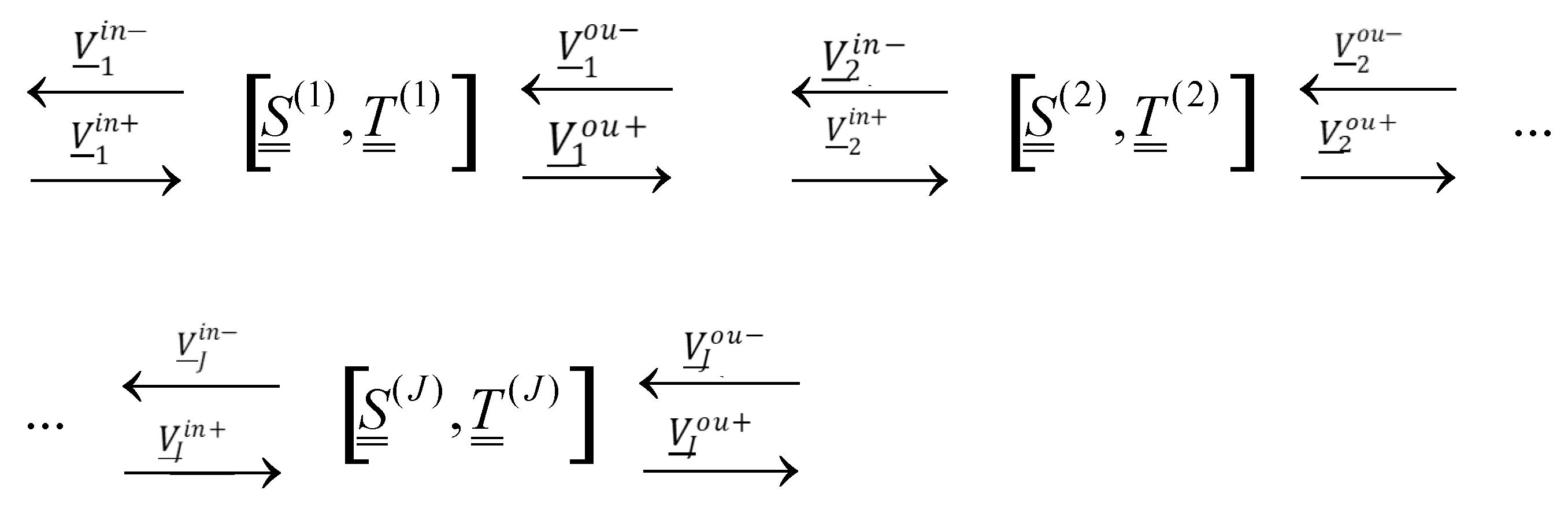
relating the coefficients of the field distribution incident (in) on the antenna structure with the coefficients of the field distribution generated by this antenna (ou—the sum of the reflected and scattered fields), see Figure 2.

$$\left[\begin{array}{c}{\underset{\_}{V}}^{ou+}\\ {\underset{\_}{V}}^{ou-}\end{array}\right]=\left[\begin{array}{cc}{\underset{\_}{\underset{\_}{S}}}_{11}& {\underset{\_}{\underset{\_}{S}}}_{12}\\ {\underset{\_}{\underset{\_}{S}}}_{21}& {\underset{\_}{\underset{\_}{S}}}_{22}\end{array}\right]\hspace{0.33em}\left[\begin{array}{c}{\underset{\_}{V}}^{in-}\\ {\underset{\_}{V}}^{in+}\end{array}\right]$$

(146)

The signs “+”, “−” indicate propagation in the direction consistent with or opposite to the sense of the z-axis. In the case of field incidence in the half-space z > 0 analyzed above, the elements of the “input” (in) and “output” (ou) vectors are, respectively, as follows:

$${\underset{\_}{V}}^{in-}={\underset{\_}{V}}^i$$

(147)

$${\underset{\_}{V}}^{in+}=0$$

(148)

$${\underset{\_}{V}}^{ou+}={\underset{\_}{V}}^s+\underset{\_}{\Gamma }{\underset{\_}{V}}^i$$

(149)

$${\underset{\_}{V}}^{ou-}=0$$

(150)

The signs “+”, “−“ indicate propagation in the direction of and are expressed by the coefficients of the distribution ${\nu }_{k }^i \mathrm{and} {\nu }_k^s$ of the incident field and the scattered field on the complete system of Floquet harmonics of the periodic antenna structure.

Symbols $\hspace{0.33em}{\underset{\_}{\underset{\_}{S}}}^{\left(J\right)}$, $\hspace{0.33em}{\underset{\_}{\underset{\_}{T}}}^{\left(J\right)}$ denote the scattering and transmission matrix of the planar element of the layered structure, respectively, and the index $J$ denotes the number of elements of the layered structure.

The elements of the scattering matrix depend exclusively, through the matrix of reflection coefficients Γ, Green’s function G and the form of Floquet harmonics ψ_k, on the geometry and material parameters of the antenna structure as well as on the system of basic (testing) functions φ_q adopted in the analysis. By the very definition of the scattering matrix, its elements do not depend on the specifically analyzed case of excitation of the antenna structure and on the currents induced on its elements. Thus, the scattering matrix completely characterizes the antenna structure in the general case for any of its excitations. Its construction, carried out in the spectral space spanned by the Floquet harmonic system, allows the analysis of any periodic antenna structure placed on a multilayer dielectric substrate, through cascading composition of scattering matrices corresponding to its individual layers. The description of the periodic antenna structure unrestricted in the (x,y) plane through the scattering matrix defined in this way also allows the analysis to be generalized to the case of a periodic structure with finite dimensions.

4. Dissipation Radiation Field Analysis of Antenna Array of Limited Dimensions

4.1. Antenna Area Limited Features

We consider the case of a limited periodic antenna array in plane z = 0 in the directions of the x- and y-axes. The antenna array is immersed in any unconfined dielectric medium, layered in planes perpendicular to the z-axis and placed on the boundary of two layers or dielectric media; in the special case, in free space. The antenna cells with the carrier function h_mn cover the part of the plane z = 0 corresponding to the carrier function H_MN(x,y):

$${\sum }_{m,n}{h}_{mn}(x,y)=H_{MN}(x,y),$$

(151)

where

$$H_{MN}\left(x,y\right)=1 for x\in \left[-M{d}_x,M{d}_x\right]\mathit{and}y\in \left[-N{d}_{y}N{d}_y\right]$$

(152)

$$H_{MN}\left(x,y\right)=o for x\notin \left[-M{d}_x,M{d}_x\right]\mathit{or}y\notin \left[-N{d}_{y}N{d}_y\right]$$

(153)

where integers m, n number the cells in the x-axis direction m = −M, −M + 1, …, 0, …, M − 1, M and in the y-axis direction n = −N, −N + 1, …, 0, …, N − 1, N. The metallized elements of the antenna are distributed periodically in the same limited area of the z = 0 plane in individual cells of the grid (m,n) and cover the area with the carrier function A_MN(x,y):

$${\sum }_{m,n}{a}_{mn}\left(x,y\right)=A\left(x,y\right)H_{MN}\left(x,y\right)=A_{MN}(x,y)$$

(154)

Note that the functions H_MN(x,y), A_MN(x,y) factorize into components depending on x and y:

$$H_{MN}(x,y)=H_{MNx}\left(x\right)H_{MNy}\left(y\right),$$

(155)

$$A_{MN}\left(x,y\right)=A_{MNx}\left(x\right)A_{MNy}\left(y\right).$$

(156)

Due to the antenna limitation in the plane z = 0, the antenna cells are distinguished, e.g., in the solution of the scattering problem, by their position relative to the origin of the coordinate system (x,y) = (0,0), assumed as the center point of the central cell (0,0). However, in this case the solution (current distribution) changes from cell to cell. In an unconstrained periodic system, each cell (m,n) can be a central cell. In a constrained periodic system, the central cell is uniquely determined by its position in the center of the antenna grid area; each cell other than the central one (m,n) is uniquely determined by the position of its center relative to the center of the grid area (x,y) = (0,0). For further considerations, it is therefore necessary to define the carrier (window) function H_MNmn(x,y) of the antenna grid with the origin of the coordinate system at points (x_m,y_m) of subsequent cells (m,n). The H_MNmn(x,y) functions change depending on the hypothetical cell in which the origin of the coordinate system is located and are defined by translations by the vector (x_m,y_n) = (md_x,nd_y) of the H_MN: function:

$$H_{mn}(x,y)=H_{00}(x-x_m,y-y_m)=H_{MN}(x-x_m,y-y_m).$$

(157)

Their Fourier transforms are, respectively, as follows:

$$F(H_{00})(k_x,k_y)={\displaystyle \frac{MN{d}_x{d}_y}{{\pi }^2}}{\displaystyle \frac{\mathit{sin}M{k}_x{d}_x}{M{d}_x}}{\displaystyle \frac{\mathit{sin}N{k}_y{d}_y}{N{d}_y}},$$

(158)

$${\overline{H}}_{ook}\equiv {\overline{H}}_{MN00}(k_{xk},k_{yk})=(d_x{d}_y{)}^{-1}F(H_{00})(k_{xk},k_{yk})={\displaystyle \frac{MN}{{\pi }^2}}{\displaystyle \frac{\mathit{sin}M{k}_{xk}{d}_x}{M{d}_x}}{\displaystyle \frac{\mathit{sin}N{k}_{yk}{d}_y}{N{d}_y}},$$

(159)

$$\begin{array}{c}{\overline{H}}_{mnk}\equiv {\overline{H}}_{mn}(k_{xk},k_{yk})={\overline{H}}_{00}(k_{xk},k_{yk})\mathit{exp}\left[-i\left(m{k}_{xk}{d}_x+n{k}_{yk}{d}_y\right)\right]\\ \hspace{0.33em}={\overline{H}}_{00}(k_{xk},k_{yk})\mathit{exp}\left[-i\left(m{\varphi }_{xk}+n{\varphi }_{ky}\right)\right].\end{array}$$

(160)

Therefore, the Fourier transforms of the cell carrier function experience a phase modulation equal to the phase modulation of the corresponding Floquet harmonics of the incident field.

4.2. Solution to Distraction Problem

Due to the general form of the formulation of the scattering problem on an unconstrained antenna array—defining the scattering matrix of the grid in the spectral space spanned by the full harmonic system—generalizing, using the above-defined window functions, the solution procedure for the case of an array of constrained dimensions does not pose any major difficulties. Only the initial equations containing the current distribution change:

$$\underset{\_}{J}(x,y)=H_{mn}(x,y){\sum }_q{\underset{\_}{j}}_q{\underset{\_}{\varphi }}_q(x,y)={\sum }_k{\overline{\underset{\_}{J}}}_k{\overline{H}}_{mnk}{e}_k(x,y),$$

(161)

$${\underset{\_}{E}}^s\left(x,y,0\right)=\left(\underset{\_}{G}\ast \underset{\_}{J}\ast H_{mn}\right)\left(x,y\right)={\sum }_k{\overline{\underset{\_}{G}}}_k{\overline{\underset{\_}{J}}}_k{\overline{H}}_{mnk}{e}_k(x,y)$$

(162)

where

$${\overline{\underset{\_}{J}}}_k={\sum }_q{\underset{\_}{j}}_q{\overline{\underset{\_}{\varphi }}}_{qk}$$

(163)

by multiplying the amplitudes of their spectral representations by the Fourier transform of the window function ${\overline{H}}_{mnk}$ corresponding to the selected cell (m,n). Each cell (m,n) corresponds to a different form of the window function H_mn(x,y) due to its location relative to the central point of the window function carrier H_MN(x,y). For each pair of numbers (m,n), a different solution is obtained defining the distribution of currents on the surface of the metallized part of the cell (m,n). From a formal point of view, the formulation and solution of the problem of scattering on an antenna array of limited size should take into account the continuous spectrum of wave number values k in the spectral distributions of field quantities and currents, i.e., the continuous Fourier transform should be used instead of spectral distributions at points corresponding to discrete values of wave numbers of successive Floquet harmonics. The numerical solution of the problem formulated in this way would also in this case reduce the analyzed problem to a problem with a discrete spectrum, imposed by numerical procedures of the fast Fourier transform (FFT) type. Hence, it seems justified to use spectral distributions of the analyzed quantities with a spectrum determined by harmonics corresponding to the case of an unconstrained periodic structure. Thus, in terms of the formal notation of equations, except for the modification in the above equations by introducing a window function, the formulation and solution of the posed scattering problem on an infinite periodic antenna structure consist of the decomposition of the basic functions, currents and fields into Floquet harmonics, in a way analogous to the unconstrained antenna grid analyzed in the previous chapter.

$${\underset{\_}{\varphi }}_q(x,y)={\sum }_k{\overline{\underset{\_}{\varphi }}}_{qk}{\underset{\_}{\Psi }}_k(x,y),$$

(164)

$$\underset{\_}{J}(x,y)={\sum }_{q,k}{\underset{\_}{j}}_q{\overline{\underset{\_}{\varphi }}}_{qk}{\overline{H}}_{mnk}{e}_k(x,y),$$

(165)

$${\underset{\_}{E}}_t^i(x,y,0)={\sum }_k{v}_k^i{\underset{\_}{\Psi }}_k(x,y),$$

(166)

$${\underset{\_}{E}}_t^e(x,y,0)={\sum }_k(1\pm {\Gamma }_k)v_k^i{\underset{\_}{\Psi }}_k(x,y),$$

(167)

$${\underset{\_}{E}}_t^s(x,y,0)={\sum }_k{v}_k^s{\underset{\_}{\Psi }}_k(x,y).$$

(168)

By relating the scattered field to the induced currents using Green’s function,

$${\underset{\_}{E}}_{tmn}^s\left(x,y,0\right)={\sum }_k{\overline{\underset{\_}{G}}}_k{\underset{\_}{\overline{J}}}_k{\overline{H}}_{mnk}{e}_k(x,y)$$

(169)

and imposing, using the Galerkin method, the condition of zeroing of the total field on the surface of the antenna’s metal elements on the representation of the field and induced currents:

$${\underset{\_}{E}}_{tmn}(x,y,0)A_{MN}=\left({\underset{\_}{E}}_t^e(x,y,0)+{\underset{\_}{E}}_{tmn}^s(x,y,0)\right)A_{MN}=0$$

(170)

As a result, we obtain a system of two matrix algebraic equations:

$$\underset{\_}{W}\hspace{0.33em}\underset{\_}{j}={\underset{\_}{V}}^s$$

(171)

$$\underset{\_}{N}\hspace{0.33em}{\underset{\_}{V}}^i=-\underset{\_}{U}\underset{\_}{j}$$

(172)

where, respectively,

$$[\underset{\_}{W}{]}_{kqj}\equiv W_{kqj}={\sum }_i{\psi }_{ki}^{\ast }{\overline{G}}_{kij}{\overline{\varphi }}_{qkj}{\overline{H}}_{mnk}$$

(173)

$${\left[\underset{\_}{N}\right]}_{qkj}\equiv N_{qkj}=(1+{\Gamma }_k){\overline{\varphi }}_{qkj}^{\ast }{\psi }_{kj}$$

(174)

$${\left[\underset{\_}{U}\right]}_{pqij}\equiv U_{pqij}={\sum }_k{\overline{\varphi }}_{pki}^{\ast }{\overline{G}}_{kij}{\overline{\varphi }}_{qkj}{\overline{H}}_{mnk}$$

(175)

$${\left[j\right]}_{qj}\equiv j_{qj}$$

(176)

$${\left[V^s\right]}_k\equiv {\nu }_k^s$$

(177)

$${\left[{\underset{\_}{V}}^i\right]}_k\equiv {\nu }_k^i$$

(178)

$${\left[j\right]}_{qxmn}\equiv j_{qxmn}$$

(179)

$${\left[j\right]}_{qymn}\equiv j_{qymn}$$

(180)

in the cell defined by the indices of the window function H_mn. By solving the above system of algebraic equations for subsequent window functions H_mn, we obtain the distribution of current J_mn on subsequent cells (m,n) of the limited periodic antenna array, i.e., we obtain M × N solutions of the above system of equations for M × N waveforms of the function H_mn(x,y). The total distribution of currents on all cells simultaneously can be presented in the following form:

$$\underset{\_}{J}\left(x,y\right)={\sum }_{m,n}{\underset{\_}{J}}_{mn}{\left(xy\right)a}_{mn}(x,y).$$

(181)

where

$$\underset{\_}{J}\left(x,y\right)={\sum }_q{\underset{\_}{J}}_q{\underset{\_}{\Phi }}_q\left(x,y\right)={\sum }_k{\overline{\underset{\_}{J}}}_k{e}_k\left(x,y\right)={\sum }_k{\sum }_q{\overline{\underset{\_}{\varphi }}}_{qk}{\underset{\_}{j}}_q{e}_k(x,y),$$

(182)

The final solution, however, requires an unambiguous connection of the current distribution with the incident and scattered fields:

$${\underset{\_}{V}}^s=-\underset{\_}{W}\hspace{0.33em}{\underset{\_}{U}}^{-1}\hspace{0.33em}\underset{\_}{N}\hspace{0.33em}{\underset{\_}{V}}^i$$

(183)

That is, it requires a single, unique solution to the above system of equations, considering the current distributions on all antenna cells simultaneously. Let us note that the presented construction of the solution does not exclude another, arbitrary form of the window function H_mn(x,y) defined by its amplitude and phase changing from point to point. A vector form of this function is also possible. Thus, the final solution to the problem under consideration can be obtained by imposing on the window function a modulation in phase and amplitude reproducing the changes in the current distribution when passing from cell to cell. For this purpose, we construct another window function H⁽⁰⁾_MN with the amplitudes of the distribution determined symbolically by the system of equations in the spectral space:

$${\overline{\underset{\_}{H}}}_{MNk}^{\left(0\right)}=a_k^{\left(0\right)}{\overline{H}}_{MNk}{\overline{\underset{\_}{J}}}_k,$$

(184)

with the appropriate normalization factor a_k⁽⁰⁾, satisfying the condition for each pair of numbers (m,n). Then, in the final formally exact solution, the current distribution coefficients ${\overline{\underset{¯}{J}}}_k$ should no longer depend on the position of the analyzed antenna cell.

By introducing the thus defined window functions 184 and 185 into the solution procedures 171 and 172, we obtain the following:

$${\underset{\_}{\varphi }}_q(x,y)={\sum }_k{\overline{\underset{\_}{\varphi }}}_{qk}{\underset{\_}{\Psi }}_k(x,y),$$

(185)

$$\underset{\_}{J}(x,y)={\sum }_{q,k}{\underset{\_}{j}}_q{\overline{\underset{\_}{\varphi }}}_{qk}{\overline{\underset{\_}{H}}}_{mnk}^{\left(0\right)}{e}_k(x,y),$$

(186)

$${\underset{\_}{E}}_t^i(x,y,0)={\sum }_k{v}_k^i{\underset{\_}{\Psi }}_k(x,y),$$

(187)

$${\underset{\_}{E}}_t^e(x,y,0)={\sum }_k(1\pm {\Gamma }_k)v_k^i{\underset{\_}{\Psi }}_k(x,y),$$

(188)

$${\underset{\_}{E}}_t^s(x,y,0)={\sum }_k{v}_k^s{\underset{\_}{\Psi }}_k(x,y).$$

(189)

$$\underset{\_}{\underset{\_}{W}}\hspace{0.33em}\underset{\_}{j}=\hspace{0.33em}{\underset{\_}{V}}^s,$$

(190)

$$\underset{\_}{\underset{\_}{N}}\hspace{0.33em}{\underset{\_}{V}}^i=-\underset{\_}{\underset{\_}{U}}\hspace{0.33em}\underset{\_}{j},$$

(191)

Substituting into 171 and 172, we obtain the following equations:

$${\left[\underset{\_}{W}\right]}_{kqj}\equiv W_{kqj}={\sum }_i{\psi }_{ki}^{\ast }{\overline{G}}_{kij}{\overline{\varphi }}_{qkj}{\overline{H}}_{mnkj}^{\left(0\right)},$$

(192)

$${\left[\underset{\_}{N}\right]}_{qkj}\equiv N_{qkj}=(1+{\Gamma }_k){\overline{\varphi }}_{qkj}^{\ast }{\psi }_{kj},$$

(193)

$${\left[\underset{\_}{U}\right]}_{pqij}\equiv U_{pqij}={\sum }_k{\overline{\varphi }}_{pki}^{\ast }{\overline{G}}_{kij}{\overline{\varphi }}_{qkj}{\overline{H}}_{mnkj}^{\left(0\right)},$$

(194)

which, when solved, we obtain the distribution of currents J⁽⁰⁾(x,y). Returning to the repeated determination of the modified window function

$${\overline{\underset{\_}{H}}}_{MNk}^{\left(1\right)}=a_k^{\left(1\right)}{\overline{H}}_{MNk}^0{\overline{\underset{\_}{J}}}_k,$$

(195)

we obtain an iterative sequence as a result:

$${\underset{\_}{H}}_{MN}^{\left(0\right)}(x,y),{\underset{\_}{H}}_{MN}^{\left(1\right)}(x,y),{\underset{\_}{H}}_{MN}^{\left(2\right)}(x,y),\dots \dots .$$

(196)

$${\underset{\_}{J}}^{\left(0\right)}(x,y),{\underset{\_}{J}}^{\left(1\right)}(x,y),{\underset{\_}{J}}^{\left(2\right)}(x,y),$$

(197)

where in the limit the window and current distribution functions should have the same course:

$${\underset{\_}{H}}_{MN}^{\left(\alpha \right)}(x,y)={\underset{\_}{J}}^{\left(\alpha \right)}(x,y)\times const.$$

(198)

The sign “∞“ seems to have a purely theoretical meaning here because satisfactory, sufficiently accurate results should be given already by the zeroth iteration step, where the solution of the problem for any cell (m,n) should no longer depend significantly on the numbers m,n. This would mean that already in the zeroth iteration step would be enough to solve the system of equations only for the central cell (m,n) = (0,0), and the changes in the distribution of currents J⁽⁰⁾(x,y) on other cells should be precisely simulated by the distribution of the window function H⁽⁰⁾_MN(x,y). This in turn allows us to construct the relationship between the scattered and incident fields:

$${\underset{\_}{V}}^s=-\underset{\_}{W}\hspace{0.33em}{\underset{\_}{U}}^{-1}\hspace{0.33em}\underset{\_}{N}\hspace{0.33em}{\underset{\_}{V}}^i$$

(199)

$$\left[\begin{array}{cc}{\underset{\_}{V}}^{S+}& +\underset{\_}{\underset{\_}{\Gamma }}{\underset{\_}{V}}^{i-}\\ {\underset{\_}{V}}^{S-}& -\underset{\_}{\underset{\_}{\Gamma }}{\underset{\_}{V}}^{i+}\end{array}\right]=\left[\begin{array}{cc}{\underset{\_}{\underset{\_}{S}}}_{11}& {\underset{\_}{\underset{\_}{S}}}_{12}\\ {\underset{\_}{\underset{\_}{S}}}_{21}& {\underset{\_}{\underset{\_}{S}}}_{22}\end{array}\right]\hspace{0.33em}\left[\begin{array}{c}{\underset{\_}{V}}^{i-}\\ {\underset{\_}{V}}^{i+}\end{array}\right]$$

(200)

finally illustrating the complete solution of the scattering problem analyzed.

I.

Solving M × N systems of algebraic equations with a window function in the form (171 ÷ 172) separately for each cell (m,n) of the antenna with metallization;

II.

Solving one global system of equations (190) ÷ (191) with a window function (190), (191), including determining the current distributions on all cells (m,n) with metallization simultaneously;

III.

Performing the iterative procedure (197) ÷ (198) in order to verify the accuracy of the obtained solution.

It should be emphasized that the proposed procedure allows for determining the current distribution separately in each antenna cell, considering the following:

• The influence of the remaining cells by using the method of moments separately for each cell;
• The finite dimensions of the antenna array and thus considering the edge (diffraction) effects by introducing a window function into the strict spectral representation of the scattered field.

However, the applied spectral Galerkin method enabled the transformation of this representation into a matrix system of equations. This is a proposal for an accurate and effective solution to the problem of reconnaissance on a periodic antenna array of limited size. In the available literature, there is no publication about the efficiency of the methods used.

According to the author’s knowledge, this is an original solution that has not been published anywhere. To verify the developed procedure, numerical calculations were carried out, preceded by tests checking the effectiveness and accuracy of the individual stages. Then, calculations were made for the structure shown in Figure 3. The results obtained, compared with the measurements, are shown in Figure 4, and they encourage further work in this direction, despite the very long duration of the calculations. The designed and tested antenna is a multilayer structure. The power supply system based on Wilkinson dividers was placed on a dielectric with a dielectric constant of ε_r = 4.6 and lossiness tgδ = 10⁻³. On the other side of the dielectric, we have the entire metalized surface, the surface of which acts as a screen. The radiating system was made on a dielectric with ε_r = 2.1. The thickness of both dielectrics is 1.5 mm. Such a selection of the dielectric results from the need to ensure a good fit for the surrounding space. The antenna is designed for a frequency of 3 GHz.

5. Spectral Representation of the Current Distribution on a Limited Antenna Array

The solution to the scattering problem analyzed is based on the spectral decomposition of the window function on the Floquet harmonics e_k(x,y). In general, the analysis of the problem also allows for the possibility of decomposing the window function on the harmonics of the grid with other values of the grid steps, for example, equal to Md_x and Nd_y in the x- and y-axes. In this case, this corresponds to the spectral decompositions on the harmonics of a planar rectangular unconstrained periodic structure with a single cell carrier equal to the carrier of the H_MN function. The basic relations specifying this type of spectral decompositions used in this work will be presented below. The effectiveness of the solution to the problem is conditioned by the formulation of an appropriate spectral representation of the current distribution function of the constrained periodic structure:

$${\underset{\_}{J}}_{mn}(x,y)=H_{mn}(x,y)\underset{\_}{J}(x,y)$$

(201)

in a form, analogous to the case of an unconstrained structure. The functions J_mn(x,y) and J(x,y) denote the distribution of currents on, respectively, a constrained and unconstrained periodic grid, H_mn is the window function of the constrained structure and the pair of integers m, n determines the position of the origin of the coordinate system relative to the central point (geometric center) of the constrained antenna structure.

Let us introduce the decomposition of the function J(x,y) into the Floquet harmonics of the periodic array with the array jumps equal to d_x, d_y, respectively:

$$\underset{\_}{J}(x,y)={\sum }_k{\overline{\underset{\_}{J}}}_k{e}_k(x,y),$$

(202)

where the distribution function is expressed by the Fourier transform of the function $\underset{¯}{J}(x,y)$:

$$F\left(\underset{\_}{J}\right)(k_x,k_y)={\sum }_k(d_x{d}_y{)}^{-1/2}{\overline{\underset{\_}{J}}}_k\delta (k_x-k_{xk})\delta (k_y-k_{yk}).$$

(203)

and in the spectral decomposition, we use the normalized Floquet harmonics of the periodic antenna array.

Then, we introduce the decomposition of the function H_mn(x,y) into new Floquet harmonics of the periodic grid with grid steps equal to Md_x, Nd_y, respectively:

$$H_{mn}(x,y)={\sum }_{\kappa }{\overline{H}}_{mn\kappa }{f}_{\kappa }(x,y)$$

(204)

with a distribution function defined by the Fourier transform of the window function:

$$F\left(H_{mn}\right)(k_x,k_y)={\sum }_k(M{d}_{x}N{d}_y{)}^{-1/2}{{\overline{H}}_{mn}}_k\delta (k_x-k_{x\kappa })\delta (k_y-k_{y\kappa })$$

(205)

and using Floquet harmonics with a higher spectrum sampling rate and zero phase shift in the harmonic exponent:

$$f_{\kappa }(x,y)=\left(M{d}_{x}N{d}_y{)}^{-1/2}\mathit{exp}[i\right(k_{x\kappa }x+k_{y\kappa }y\left)\right],$$

(206)

$$k_{x\kappa }=2\pi m″/M{d}_x,$$

(207)

$$k_{y\kappa }=2\pi n″/M{d}_y,$$

(208)

$$k_{0x\kappa }=0=k_{0y\kappa }.$$

(209)

Ultimately, the current distribution in the limited antenna array is expressed by the double sum of the Floquet harmonic distribution of both types:

$${\underset{\_}{J}}_{mn}(x,y)={\sum }_k{\sum }_{\kappa }{\overline{\underset{\_}{J}}}_k{\overline{H}}_{mn\kappa }{e}_k(x,y)f_{\kappa }(x,y).$$

(210)

This is the starting formula for modifying the solution of the scattering problem on an unconstrained antenna grid, where the relationship holds the following:

$$\chi =k$$

(211)

$$\underset{\_}{J}(x,y)={\sum }_k{\overline{\underset{\_}{J}}}_k{e}_k(x,y).$$

(212)

From the form of the above expressions, several parallel specifications of the numerical analysis of the solution follow. In the simple formulation of the problem, in the spectral representation of the individual quantities, one can use harmonics of the same type with common wave vectors (up to a constant phase component; for harmonics f_κ, this component is zero), that is, either

Case 1:

$$k_{x\kappa }-k_{0x\kappa }=2\pi m″/M{d}_x$$

(213)

$$k_{y\kappa }-k_{0y\kappa }=2\pi n″/M{d}_y$$

(214)

Or case 2:

$$k_{xk}-k_{0xk}=2\pi m^{\prime }/d_x$$

(215)

$$k_{yk}-k_{0yk}=2\pi n^{\prime }/d_y$$

(216)

In the first case, the number of harmonics necessary to sample the current distribution spectrum is larger M × N times than in the second case, which may be important due to limitations in the time of performing numerical calculations and available RAM. We focus on the second case, which does not exclude later generalization of the method to a more accurate case in numerical calculations due to the higher sampling density of the current function. In this case, we obtain the following:

$${\underset{\_}{J}}_{mn}(x,y)={\sum }_k{\sum }_{k^{\prime }}{\overline{\underset{\_}{J}}}_k{\overline{H}}_{mn{k}^{\prime }}{e}_k(x,y)f_{k^{\prime }}(x,y)$$

(217)

where $k\equiv \hspace{0.33em}\left\{m^{\prime },n^{\prime },l\right\}$, $k^{\prime }\equiv \left\{m″,n^{″},l \right\}.$ From the assumed form of harmonics, it follows:

$$e_k(x,y)f_{k^{\prime }}(x,y)=\left(d_x{d}_y{)}^{-1/2}{e}_{k″}\right(x,y)$$

(218)

where $k″\equiv \left\{m^{\prime }+m″,n^{\prime }+n″,l\right\}$, and we obtain the following specification of the spectral representation of the current distribution on the antenna grid:

$${\underset{\_}{J}}_{mn}(x,y)={\sum }_{k″}{\overline{\underset{\_}{J}}}_k{\overline{H}}_{mn{k}^{\prime }}\left(d_x{d}_y{)}^{-1/2}{e}_{k″}\right(x,y)$$

(219)

The following shortened version of the above representation was adopted:

$$\underset{\_}{J}(x,y)={\sum }_k{\overline{\underset{\_}{J}}}_k{\overline{H}}_{mnk}{e}_k(x,y)$$

(220)

where the individual designations are understood as follows:

$$\underset{\_}{J}(x,y)\equiv {\underset{\_}{J}}_{mn}(x,y)$$

(221)

$${\overline{\underset{\_}{J}}}_k\equiv {\overline{\underset{\_}{J}}}_k$$

(222)

$${\overline{H}}_{mnk}\equiv {\overline{H}}^{\prime }(d_x{d}_y{)}^{-1/2}$$

(223)

$$e_k(x,y)\equiv e_{k^{\prime }}(x,y)$$

(224)

In the first case, i.e., with denser sampling of the current distribution spectrum, we proceed analogously with the above sequence of definitions of individual spectral quantities. It should be noted here that, in general, the presented solution method also allows for the possibility of direct use of the spectral distribution with simultaneous use of Floquet harmonics.

6. Conclusions

Printed antennas have been some of the most innovative areas of antenna technology for a dozen or so years. They are increasingly used in antenna arrays. However, the dielectric substrate used promotes the excitation of surface waves, which, propagating along the dielectric plane, disrupts the normal operation of the antenna. Therefore, an important issue is the choice of method for their analysis. Among the methods of analyzing microstrip antennas, the method of integral equations is considered to be the most accurate. Commonly used methods for constructing approximate solutions of antenna theory equations are direct methods, consisting in reducing an integral equation or a system of integral equations to a system of linear algebraic equations. Many methods of algebraization are known, with the vast majority being, in fact, different variants of one general scheme, which in the technical literature has been assumed, following Harrington, to be called the method of moments. The method of moments offers many effective computer-implementable algorithms for solving integral equations, which is why it quickly became almost mandatory in solving problems of radiation and diffraction of electromagnetic waves on thin wires, and phenomena related to antenna radiation and coupling between them. Planar, multilayer, periodic dielectric structures are currently widely used in millimeter and microwave antenna technology, mainly due to their frequency and polarization selectivity properties. Antenna arrays most often consist of repeating metal radiation elements placed on or buried in a dielectric multilayer medium. Changes in the size and shape of individual antenna elements enable effective modeling of its spectral characteristics; these changes can be additionally modeled by selecting geometric and physical parameters of the dielectric layered substrate and coating. Generalized spectral analysis of the unconstrained antenna case is particularly convenient when using the window function due to the full Floquet harmonic system used in solving the problem. The proposed sequence of successive solution steps should lead to a strictly numerically convergent solution. According to the procedure given above, it is practically necessary to determine partial and global transmission matrices in order to determine the scattering matrix. In the case of specific antenna structures, various modifications of the above analysis are used to obtain faster convergence of the applied numerical procedure and to reduce the requirements of the memory capacity used by the numerical program. The selection of the number of K harmonic cutoffs included in the numerical calculations and their order in the field distribution series, is extremely important from the point of view of the effectiveness and accuracy of the procedure. The presented procedure for solving the scattering of the electromagnetic field on the antenna system is an original solution.

References

1. Kong, J.A. Electromagnetic Wave Theory; EMW Publishing: Cambridge, MA, USA, 2008. [Google Scholar]
2. Oppenheim, A.V.; Schafer, R.W. Electromagnetic Field Theory Discrete-Time Signal Processing; Pearson Education: London, UK, 2014. [Google Scholar]
3. Aourik, S.; Erkik, A.; Oukaira, A.; Dhaou, S.; Jamal, Z.; Lakhssassi, A. An Advanced Array Configuration Antenna Based on Mutual Coupling Reduction. Electronics 2023, 12, 1707. [Google Scholar] [CrossRef]
4. Liu, S.; Sun, S.; Chew, W.C. A potential-based integral equation method for low-frequency electromagnetic problems. IEEE Trans. Antennas Propag. 2018, 66, 1413–1426. [Google Scholar] [CrossRef]
5. Bender, C.M.; Orszag, S.A. Advanced Methods for Scientists and Engineers I: Asymptotic Methods and Perturbation Theory; Springer Science & Business Media: Berlin/Heidelberg, Germany, 2013. [Google Scholar]
6. Courant, R.; Hilbert, D. Methods of Mathematical Physics: Partial Differential Equations; John Wiley & Sons: Hoboken, NJ, USA, 2008. [Google Scholar]
7. Noda, T.; Yokoyama, S. Thin Wire Representation in Finite Difference Time Domain Surge Simulation. IEEE Trans. Power Deliv. 2002, 17, 840–847. [Google Scholar] [CrossRef]
8. Balanis, C. Advanced Engineering Electromagnetics; Wiley: Hoboken, NJ, USA, 2012. [Google Scholar]
9. Chew, W.C.; Sha, W.; Dai, Q.I. Green’s dyadic, spectral function, local density of states, and fluctuation dissipation theorem. arXiv 2015, arXiv:1505.01586. [Google Scholar] [CrossRef]
10. Yaghjian, A.D. Reflections on Maxwell’s treatise. Prog. Electromagn. Res. 2014, 149, 217–249. [Google Scholar] [CrossRef]
11. Qian, J.-F.; Gao, S.; Sanz-Izquierdo, B.; Wang, H.; Zhou, H.; Xu, H. Mutual Coupling Suppression Between Two Closely Placed Patch Antennas Using Higher-Order Modes. IEEE Trans. Antennas Propagat. 2023, 71, 4686–4694. [Google Scholar] [CrossRef]
12. Oltman, G.H. Electromagnetically coupled microstrip dipoles. IEEE Trans. Antennas Propag. 1981, 29, 151–157. [Google Scholar] [CrossRef]
13. Chew, W.C. Lectures on Theory of Microwave and Optical Waveguides. for ECE 531 at UIUC. 2016. Available online: https://engineering.purdue.edu/wcchew/course/tgwAll20160215.pdf (accessed on 9 July 2025).
14. Sadiku, M.N. Elements of Electromagnetics; Oxford University Press: Oxford, UK, 2014. [Google Scholar]
15. Cameron, T.R.; Eleftheriades, G.V. Analysis and characterization of a wide-angle impedance matching metasurface for 277 dipole phased arrays. IEEE Trans. Antennas Propag. 2015, 63, 3928–3938. [Google Scholar] [CrossRef]
16. Fang, D.G. Antenna Theory and Microstrip Antennas; CRC Press: Boca Raton, FL, USA, 2010. [Google Scholar]
17. Asada, T.; Baba, Y.; Nagaoka, N.; Ametani, A. An Improved Thin Wire Representation for FDTD Transient Simulations. IEEE Trans Electromagn. Compat. 2015, 57, 484–487. [Google Scholar] [CrossRef]
18. Barbuto, M.; Hamzavi-Zarghani, Z.; Longhi, M.; Monti, A.; Ramaccia, D.; Vellucci, S.; Toscano, A.; Bilotti, F. Metasurfaces 3.0: A New Paradigm for Enabling Smart Electromagnetic Environments. IEEE Trans. Antennas Propag. 2022, 70, 8883–8897. [Google Scholar] [CrossRef]
19. González, J.M.F.; Alonso, J.M.I.; Trujillo, J.G.G.; de Toca, A.N.S.; Pérez, M.S. GEODA-SARAS: Multi-Phased Array Planar Antenna Design and Measurements. Proc. Eur. Conf. Antenn. 2014, 423–425. [Google Scholar]
20. Wnuk, M. Multilayer Dielectric Periodic Antenna Structure in a Cascade View. Appl. Sci. 2022, 12, 4185. [Google Scholar] [CrossRef]
21. Sehrai, D.A.; Khan, J.; Abdullah, M.; Asif, M.; Alibakhshikenari, M.; Virdee, B.; Shah, W.A.; Khan, S.; Ibrar, M.; Jan, S.J.S.R. Design of high gain base station antenna array for mm-wave cellular communication systems. Sci. Rep. 2023, 13, 4907. [Google Scholar] [CrossRef] [PubMed]
22. Elhefnawy, M. Design and simulation of an analog beamforming phased array antenna. Int. J. Electr. Comput. Eng. 2020, 10, 1398–1405. [Google Scholar] [CrossRef]
23. Sun, L.; Li, Y.; Zhang, Z.; Wang, H. Antenna Decoupling by Common and Differential Modes Cancellation. IEEE Trans. Antennas Propagat. 2021, 69, 672–682. [Google Scholar] [CrossRef]
24. Dong, Y.; Cai, X.; Geyi, W. A Pattern Shaping Method for Focused Antenna Arrays. IEEE Antennas Wirel. Propag. Lett. 2024, 23, 1236–1240. [Google Scholar] [CrossRef]
25. Zhang, R.; Shim, B.; Wu, W. Direction-of-arrival estimation for large antenna arrays with hybrid analog and digital architecture. IEEE Trans. Signal Process. 2021, 70, 72–88. [Google Scholar] [CrossRef]
26. Zhang, A.; Wei, K.; Guan, Q.; Hu, Y. Compactly Placed High-Isolated Antenna Pair with Independent Control of Decoupling Amplitude and Phase. IEEE Trans. Antennas Propagat. 2023, 71, 2814–2819. [Google Scholar] [CrossRef]
27. Ma, Y.; Ma, R.; Lin, Z.; Zhang, R.; Cai, Y.; Wu, W.; Wang, J. Improving the age of information for covert communication with time-modulated arrays. IEEE Internet Things J. Electron. 2025, 14, 1718–1731. [Google Scholar] [CrossRef]
Figure 1. Periodic two-dimensional antenna system.
Applsci 15 07901 g001
Figure 2. Block diagram of a multilayer antenna.
Applsci 15 07901 g002
Figure 3. Eight-element antenna array.
Applsci 15 07901 g003
Figure 4. The radiation pattern of an antenna array.
Applsci 15 07901 g004
Disclaimer/Publisher’s Note: The statements, opinions and data contained in all publications are solely those of the individual author(s) and contributor(s) and not of MDPI and/or the editor(s). MDPI and/or the editor(s) disclaim responsibility for any injury to people or property resulting from any ideas, methods, instructions or products referred to in the content.