Non-Vertical Well Trajectory Design Based on Multi-Objective Optimization

Abstract

The optimization and control of the wellbore trajectory is one of the important technologies to improve drilling efficiency, reduce drilling cost, and ensure drilling safety in the process of modern oil and gas exploration and development. In this paper, a multi-objective wellbore trajectory optimization mathematical model is established, which takes into account the five factors of wellbore trajectory length, friction, torque, trajectory complexity, and target accuracy. A DR-NSGA-III-MGA algorithm (dynamic reference NSGA-III with multi-granularity adaptation) is proposed. By introducing multi-granularity reference vector generation and an information entropy-guided search direction adaptation mechanism, the performance of the algorithm in the complex target space is improved, and the three-stage wellbore trajectory is optimized. Simulation experiments show that the DR-NSGA-III-MGA algorithm is stable in a variety of complex problems, while maintaining good convergence, and has good generalization ability and practical application value.

1. Introduction

In recent years, scholars at home and abroad have conducted a lot of research and exploration on how to better consider the formation information for wellbore trajectory optimization. Using the knowledge of geological statistics, geophysics, rock mechanics, and other disciplines, advanced numerical simulation technology, and machine learning algorithms, a variety of wellbore trajectory optimization models have been proposed. Well trajectory planning and optimization are usually based on the construction requirements of the site to establish the corresponding planning model; then, the optimization algorithm is used to solve optimization problems. In the optimization algorithm, the algorithms for wellbore trajectory planning mainly include the genetic algorithm, particle swarm optimization algorithm, and ant colony algorithm.

The genetic algorithm (GA) was proposed by Professor John Holland and his colleagues from the University of Michigan in 1975 and was first applied in the field of pattern recognition. Because of its superior performance, it has been widely used to solve optimization problems. Liu Yusong et al. (2008) used the genetic algorithm to optimize the length of the horizontal section of a horizontal well [1]. Mohammed K. Almedallah et al. established a three-dimensional directional well trajectory based on the vector method and used the genetic algorithm (GA) and linear approximate constraint optimization (COBYLA) combined with geological modeling and logging extraction to optimize the path [2]. Sha Linxiu and Zhang Qizhi [3] et al. (2017) proposed a complex wellbore trajectory optimization method based on the adaptive quantum genetic algorithm. Their research is mainly inspired by the negative exponential characteristics of the Fibonacci sequence. FAQGA is used to optimize the actual measured well depth TMD, and parameter optimization in practical engineering is completed to realize trajectory optimization. Although their research reduces the time complexity, it increases the space complexity. Sha and Pan (2018) used the quantum genetic algorithm based on the Fibonacci sequence to achieve the optimal convergence speed of the drilling trajectory length [4]. Hossein Y et al. (2023) used the multi-objective genetic algorithm and TOPSIS method to select the best wellbore by combining information such as wellbore length [5]. Their research cases show that the ideal state of this method is close to 60%, and the effect is ideal, especially in the case of deflection. D. Davudov [6] (2024) combined the independent fast marching model with the genetic algorithm to effectively determine the well location that does not depend on the simulated operation, showing the robustness of its decision-making and accelerating the speed of well location optimization. Particle swarm optimization (PSO) is a heuristic search optimization algorithm under the intelligent optimization system. It was proposed by James Kennedy and Russell C. Eberhart [7] in 1995. Ding [8] (2004) improved the shortcomings of the particle swarm optimization algorithm; it is easy to fall into local minima by adding a penalty function in the study of non-vertical well trajectory optimization designs. Atashnezhad A and DA Wood [9] (2014) adjusted the behavior parameters of particle swarm optimization through meta-optimization to speed up the PSO process and applied it to the optimization of a deviated wellbore trajectory. Ma Yufeng et al. [10] (2017) used the particle swarm optimization algorithm to optimize the intelligent prediction method of a wellbore trajectory established by the method based on a support vector product and established the three-dimensional visualization of the wellbore trajectory through the study of computer three-dimensional graphics and visualization. Li et al. [11] (2019) combined the particle swarm optimization algorithm and analytic hierarchy process to optimize the objective function, taking into account the drilling trajectory length, torque, drilling cost, and target hit accuracy. Biswas, K [12] (2021) et al. proposed a multi-objective cellular automata model combining the grey wolf optimization and particle swarm optimization algorithm for wellbore trajectory optimization. Yousefzadeh et al. [13] (2023) combined the fast marching method (FMM) with particle swarm optimization (PSO), and discussed the optimization of wellbore trajectory parameters for vertical wells, deviated wells, and horizontal wells. Ant Colony Optimization (ACO) is also a typical heuristic search optimization algorithm. It was first proposed and widely accepted by Italian scholar Marco Dorigo [14] in the paper ‘Ant system: optimization by a colony of conforming agents’ in 1996. In order to further improve the iterative efficiency and solution accuracy of the ant colony algorithm, Liu Daohua [15] (2011) and Chen Mingjie [16] (2012) successively improved the ant colony algorithm, and proposed an ant colony hybrid algorithm based on chaos technology and an improved ant colony algorithm based on the adaptive pheromone volatilization factor. Although the research of the two people has improved the iterative efficiency of the ant colony algorithm, it is still unable to solve the huge challenges in wellbore trajectory planning. Luo Xu and Wu Xiaojun [17] (2015) introduced the basic principle and scope of application of the ant colony algorithm in detail in their published articles.

In view of this, Li [18] (2019) proposed a research project on wellbore trajectory planning based on the ant colony algorithm. Firstly, the sum of the squared increment difference of wellbore trajectory coordinates is taken as the objective function, and the azimuth range is taken as the constraint condition. Then, the continuous space is meshed, and finally, the ant colony algorithm is used to solve the problem. Although Li Chengyuan’s research shows that the ant colony algorithm has a fast convergence speed and good solution accuracy in wellbore trajectory planning, the computational efficiency of the ant colony algorithm will be reduced in the face of more complex construction scenarios.

The multi-objective optimization method of the wellbore trajectory is a technical means for the comprehensive optimization of multiple objectives (such as drilling cost, production, geological risk, etc.) faced by wellbore trajectory design in oil drilling engineering. Since there are often conflicts between these objectives, the multi-objective optimization method aims to find a set of Pareto optimal solutions to provide comprehensive support for decision-making. At present, domestic and foreign scholars mainly have used the multi-objective genetic algorithm (MOGA), second-generation non-dominated sorting genetic algorithm (NSGA-II), multi-objective particle swarm optimization (MOPSO), and other intelligent optimization algorithms in dealing with the multi-objective optimization of the wellbore trajectory. Mansouri et al. (2015) applied the multi-objective genetic algorithm to the two objective functions of wellbore length and torque to optimize the wellbore trajectory with a low risk and low cost [19]. Chandan Guria et al. (2014) used the elite non-dominated sorting genetic algorithm (NSGA-II) to optimize multi-objective drilling in an offshore oilfield with abnormal formation pressure in Louisiana. They considered several optimization objectives, namely drilling depth, drilling time, and drilling cost, and studied dual-objective and three-objective optimization problems, and obtained a set of good non-dominated optimal Pareto frontiers. According to the trade-off results, decision-makers can choose any point from the optimal Pareto boundary or the optimal Pareto surface, and therefore choose the corresponding value of the decision variable for the optimal drilling operation [20]. Huang et al. (2017) used NSGA-II to optimize the trajectory model of sidetracking horizontal wells with the goal of trajectory length and well profile energy and found that the solution was evenly distributed at the Pareto optimal frontier [21]. Zheng et al. (2019) proposed a multi-objective cellular particle swarm optimization algorithm with an adaptive neighborhood function. Then, the MOCPSO was applied with three objective functions to obtain a set of Pareto optimal solutions that are conducive to lower-risk and lower-cost wellbore trajectory design options [22]. Cheng et al. (2023) established a multi-objective optimization model of directional wells with trajectory length, torque, and strain energy as objectives, and proposed a multi-objective particle swarm optimization algorithm based on an adaptive grid (AGMOPSO) [23]. The particle flight mode of the inverse sine function of the inertia weight and the Gaussian breakthrough strategy are introduced, and a set of Pareto optimal solutions of the optimization model are obtained. Sha Linxiu and Li Wenyan [24] (2022) realized the optimization of wellbore trajectory based on the multi-objective particle swarm optimization algorithm to mutate particles. Hu et al. [25] (2024) used the wellbore energy and trajectory length as the goal of evaluating the trajectory and used the multi-objective particle swarm optimization algorithm to quickly design the optimal wellbore trajectory design parameters that meet the geological and engineering requirements, so as to improve the efficiency of eye trajectory designs. Aiming at the constraint problem of the target solution, a solution method based on the dynamic penalty function is proposed to improve the quality of the solution. This method can quickly and effectively optimize the optimal design parameters of the required trajectory by analyzing the actual wellbore entry target case of shale gas horizontal wells, which is helpful to improve the efficiency of trajectory design and reduce the economic cost and time cost of trajectory designs.

Traditional algorithms (minimum curvature method, cylindrical spiral method) have certain advantages in trajectory design. They can effectively solve single-objective or relatively simple multi-objective problems, but they are easy to fall into local extremum and cannot quickly obtain global optimal solutions. In addition, although some artificial intelligence algorithm optimization techniques can improve the search ability, there are major problems in engineering such as convergence speed and computational resource consumption.

2. Related Work

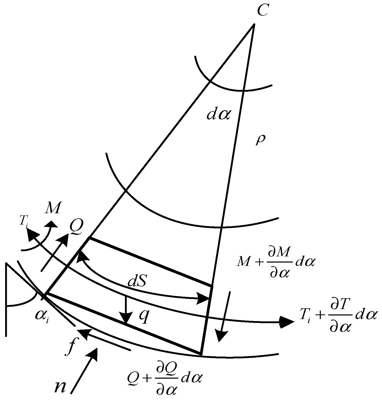
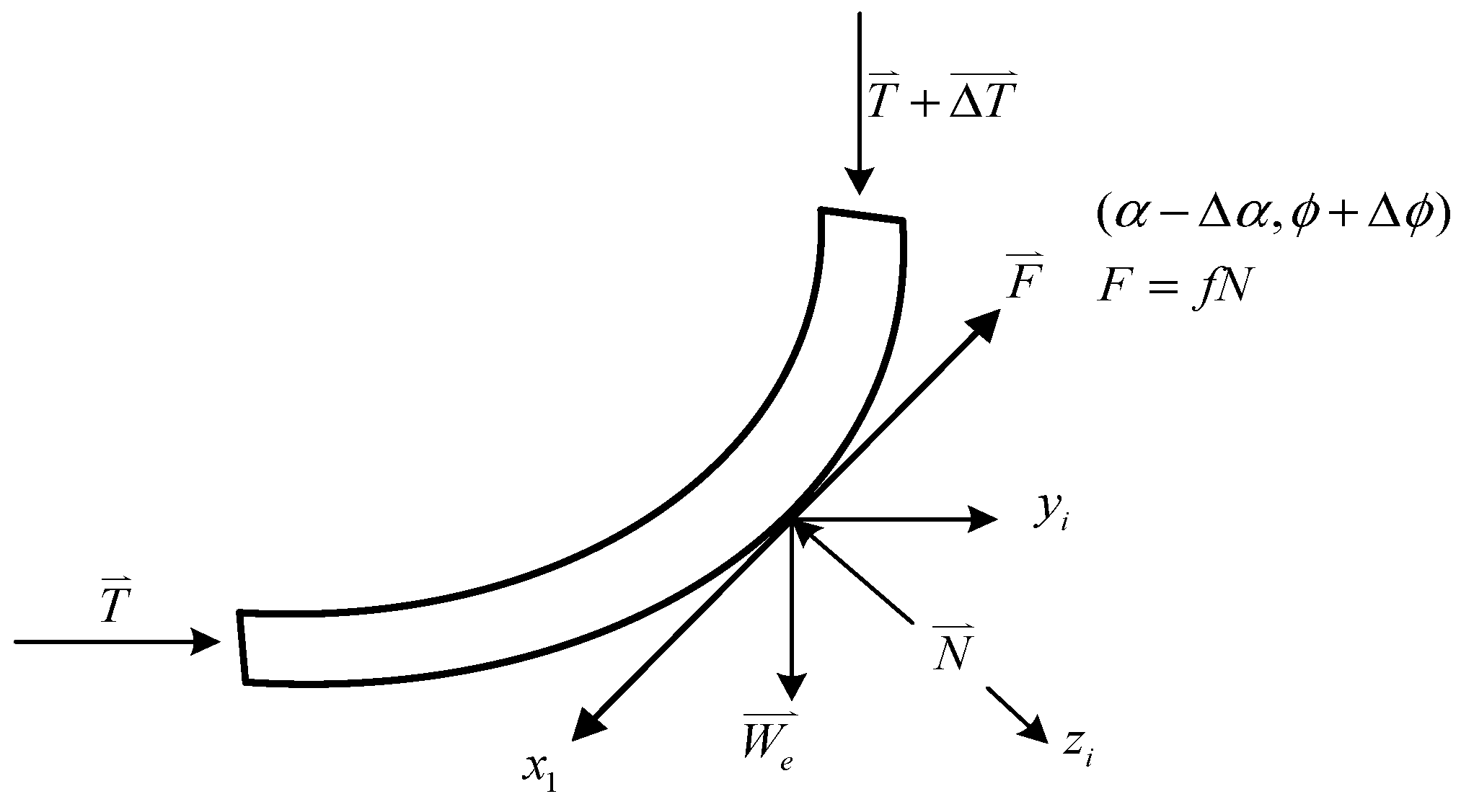
2.1. Non-Vertical Well Trajectory Classification and Characteristics Analysis

As an important part of drilling engineering, the design of a wellbore trajectory involves the knowledge of mathematics, physics, geology, and other fields. It usually includes the determination of a coordinate system, the selection of a well type, the establishment of an objective function, the selection of an optimization algorithm, and so on.

With the continuous development of the oil and gas industry, directional drilling technology is more and more widely used in complex geological conditions. As the core part of directional drilling, the wellbore trajectory design directly affects the success rate and economic benefits of drilling [26]. The following will focus on several common types of non-vertical well tracks and analyze their characteristics and applicable scenarios.

(1) Three-stage

The first type of trajectory is composed of the vertical well section, build-up section, and stable section. It is customarily called the three-section wellbore trajectory. This type of wellbore trajectory has a shallow build-up point, convenient construction, and easy control. Generally, the maximum deviation angle can be reached only in the surface casing, and then the wellbore is drilled to the bottom of the well. Due to the simple design process, this type of well trajectory is suitable for the surface layer of the geological structure and the area, which can effectively reduce the difficulty and cost of drilling construction, and the overall drilling construction process is more direct. The construction personnel can easily grasp and control the drilling parameters in the actual drilling process to ensure that the well trajectory is carried out in accordance with the design requirements. Therefore, this type of well trajectory is mainly used in traditional vertical deep vertical wells and simple directional wells.

(2) Five-stage

The second type of trajectory is composed of the vertical well section, build-up section, stable section, build-up section, and stable section, which is usually called the five-section wellbore trajectory. This kind of wellbore trajectory is mostly used for horizontal wells. The upper drilling trajectory is along the vertical deep well section, and then gradually increases the well deviation angle from the build-up section to the set maximum well deviation angle. The stable section maintains the well deviation angle in order to maintain stability to prepare for entering the increase section. Then, after increasing the inclination again in the increase section to make it close to the horizontal state, the second stable section is used to keep the wellbore at this angle until it reaches the target layer. The five-stage wellbore trajectory type is complex, but flexible, so this type of trajectory can be applied to more horizontal wells with special drilling requirements, which is conducive to achieving the maximum possible contact area with the reservoir, so as to achieve the highest production level.

(3) ‘S’ shape

The third type of trajectory is the ‘S’-shaped wellbore trajectory. This kind of wellbore trajectory is relatively shallow, and the drilling is stabilized after the surface casing is completed. The ‘S’-shaped wellbore trajectory is characterized by two build-up sections, which are similar to the ‘S’ shape. First, drilling starts from the vertical section, and then enters the first build-up section, that is, the wellbore is deviated from the vertical well trajectory. After the build-up is completed, the surface casing is cemented, and the inclined drilling is stabilized, and then the second build-up section is entered to adjust the well deviation and continue drilling. Finally, through the last stable section, the original well angle drilling is maintained, and finally the target layer is reached. The ‘S’-shaped wellbore trajectory is suitable for complex formations, and it is suitable for drilling to avoid geological conditions or multi-layer reservoirs.

In summary, the three-stage wellbore trajectory design is simple and easy to construct. It is mostly used in areas with relatively consistent geological conditions and has a high-cost performance. The five-stage wellbore trajectory has more inclined sections and stable sections, which has greater flexibility and application scope, which is conducive to the drilling of horizontal wells to maximize the contact with the reservoir area and increase the production capacity. The ‘S’-shaped wellbore trajectory double deflection design can be flexibly used to avoid obstacles or optimize the wellbore trajectory in areas with complex geological conditions or multi-reservoir drilling areas. Each type of track is based on the characteristics of its corresponding design, which is suitable for specific geological and engineering areas and has its own outstanding advantages.

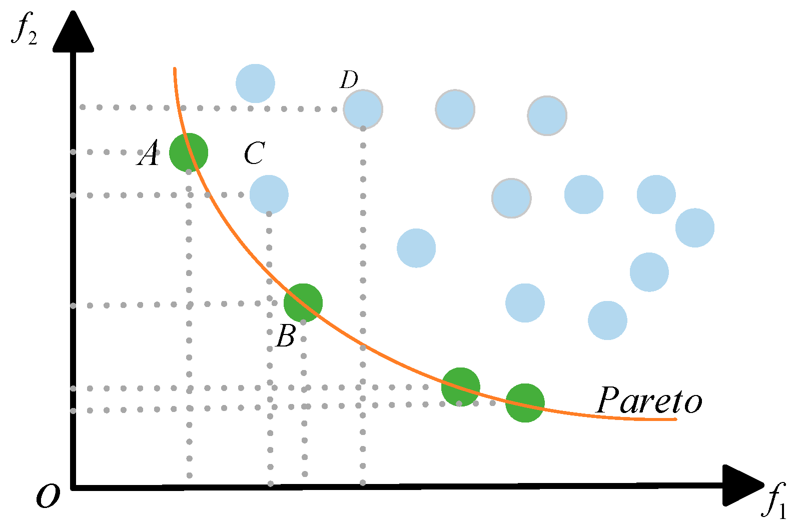
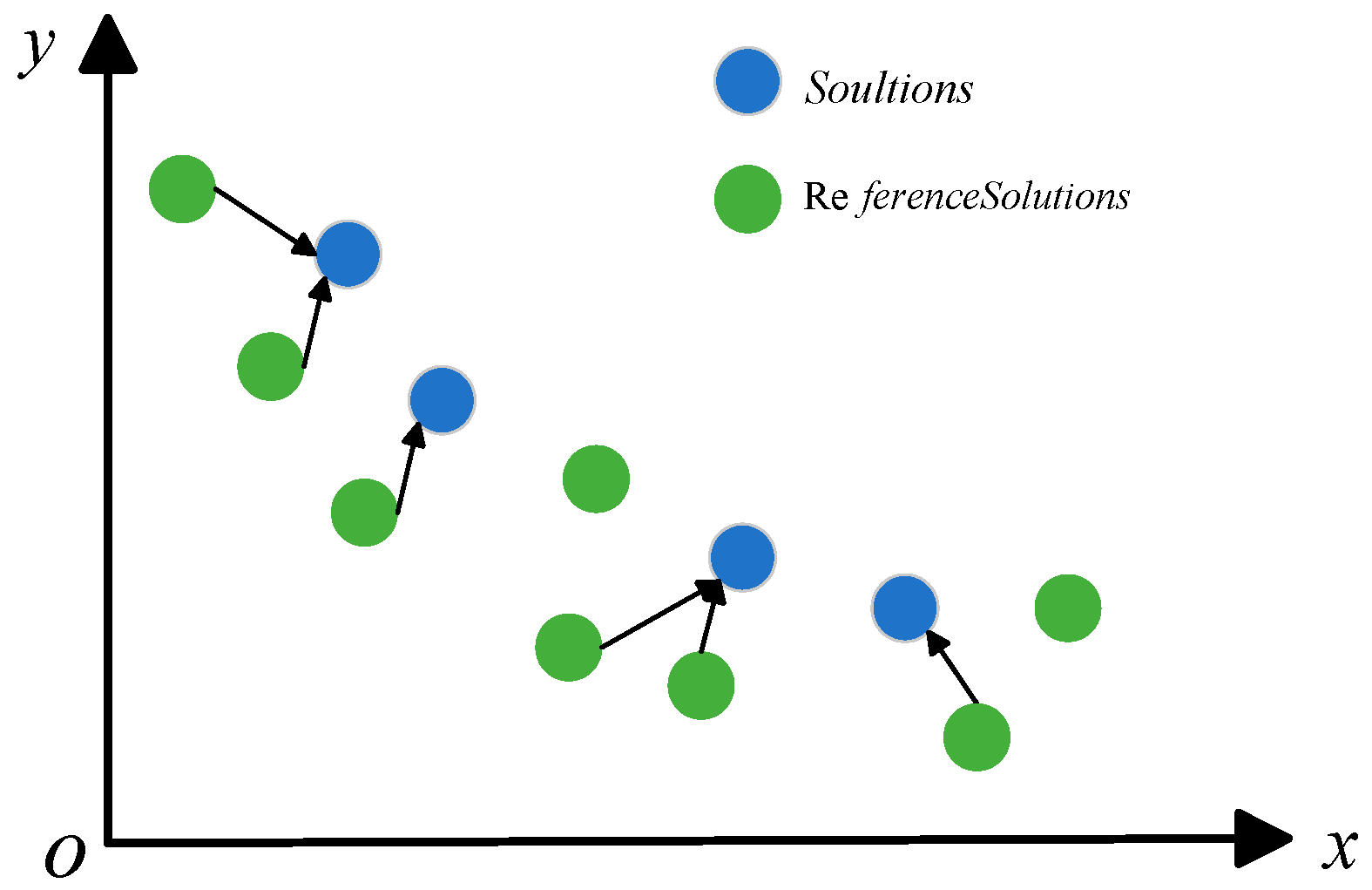
2.2. Theoretical Basis of Multi-Objective Optimization

(1) Definition of multi-objective optimization problem

In the optimization process of practical engineering problems, multi-objective optimization problems with complex and high-dimensional nonlinear constraints are often encountered [27]. There may be conflicts between different targets, which makes it very difficult to find a global optimal solution. For single-objective optimization problems, the optimal solution is usually a specific point in the solution space. In contrast, the computational complexity of multi-objective optimization problems is much higher, because it needs to satisfy multiple objective functions at the same time. In this case, there may not be a globally unique optimal solution, but rather a series of solutions that strike a balance between different objectives [28].

In a standard multi-objective optimization problem, there are usually n objective functions, m decision variables, and related constraints, which are usually expressed as shown in (1).

$$\begin{array}{c}\underset{x\in X}{\min y}=\underset{x\in X}{\min F(x)}=(f_1(x),f_2(x),\cdots ,f_n(x))\\ s.t.\left\{\begin{array}{c}{g}_i(x)\le 0 i=1,2,\cdots ,q\\ h_j(x)=0 j=1,2,\cdots ,p\end{array}\right.\end{array}.$$

(1)

Among the variables, $x=(x_1,x_2,\cdots ,x_m)\in X\subset R^m$ represents the m-dimensional decision variable vector, which constitutes the feasible region of the variable, where $X$ is the decision space; $y=(y_1,y_2,\cdots ,y_n)\in Y\subset R^n$ represents the objective function vector, where $Y$ represents the target space; $g_i\le 0 (i=1,2,\cdots ,q)$ denotes $q$ inequality constraints; and $h_j(x)=0$ represents $p$ equality constraints.

(2) Multi-objective optimization evaluation index

If for any goal i, there exists $f_i\left(x_1\right)\le f_i\left(x_2\right)$, and there exists at least one goal j such that $f_j\left(x_1\right)\le f_j\left(x_2\right)$, then the solution $x_1$ dominates the solution $x_2$ on all goals. If there is no $x$ solution dominating $x^{\ast }$, then the solution $x^{\ast }\in X_f$ is the Pareto optimal solution. The set P composed of all Pareto optimal solutions is called the Pareto optimal solution set. There is usually no obvious linear or regular functional relationship between the elements in the P set, except that they all belong to the Pareto set. The Pareto front is composed of the target vectors corresponding to all the solutions in the Pareto optimal solution set [27].

The double objective function $f_1$, $f_2$ and the minimum Pareto solution are shown in Figure 1. It can be seen from the figure that both the green point and the blue point are solutions in the feasibility region, and there is a Pareto dominance relationship between the two solutions. The performance of solution A on the two objective functions of $f_1$ and $f_2$ is better than that of solution D. At this time, solution A is called Pareto dominant solution D. Similarly, solution B and solution C are also Pareto dominant solution D. The optimal solution of the bi-objective function is on the Pareto front, and there may be multiple solutions on the front. It can be seen in the graph that the performance of solution A on the $f_1$ objective is better than that of solution B, but the performance on the $f_2$ objective is slightly worse than that of solution B. At this time, solution A is not different from solution B, and there is no Pareto dominance relationship. If there is a solution, it can Pareto dominate all other solutions, that is, it performs better than other solutions on all objective functions, which is called the absolute optimal solution. When the optimal solution does not exist, non-inferior solutions on the Pareto front are sought out, that is, Pareto optimal solutions, in order to achieve a comprehensive and effective solution to the problem [29,30].

For single-objective optimization problems, it is generally possible to determine the optimal fitness, which is usually used to evaluate its optimization effect. For multi-objective optimization problems, they need to be evaluated based on the quality of the entire solution set. In multi-objective optimization, the diversity and convergence of the solution set are two important evaluation indexes [29,30]. According to the literature statistics, there are more than 70 performance evaluation indexes, among which the most commonly used include generation distance (GD), inverse generation distance (IGD), maximum dispersion (MS), and hypervolume metric (HV).

Inverse Generational Distance (IGD) is an inverse mapping of generational distance. It is evaluated by calculating the average shortest distance between the reference point set and the approximate Pareto front solution set generated by the algorithm [31], as shown in Figure 2. IGD can simultaneously evaluate the convergence, diversity, and distribution uniformity of the algorithm. If the IGD is small, it shows that the better the convergence performance of the algorithm, the more uniform the distribution of the obtained solution set, and the larger the distance between the solution and the solution, indicating that the diversity performance is superior.

3. Establishment of Optimization Model

3.1. Selection of Optimization Index

The optimization target indexes of the wellbore trajectory used in this paper include five aspects: wellbore trajectory length, friction, torque, wellbore trajectory complexity, and target accuracy (Appendix A).

(1) Borehole trajectory length

The length of wellbore trajectory is an important index to evaluate the drilling cost. The deeper the well is drilled, the more materials are needed, the more time is spent, and the higher the energy is consumed. The wellbore trajectory is the actual path of the drill bit in the three-dimensional geological space. It is a continuous and smooth curve, which is generally divided into multiple straight lines and curves. In this paper, the wellbore trajectory is considered to be composed of straight lines and deflecting sections. The minimum curvature method is used to describe the well section. The calculation of the minimum curvature method is to form a smooth curve connection transition by ensuring that the curvature of each wellbore trajectory changes very little, so that the drilling process is more stable, which can reduce the friction and torque in the drilling process.

The calculation model of well depth $L_i$ in stable section is

$$L_i=(D_B-D_A)/\cos \alpha ,$$

(2)

where $D_A$ and $D_B$ represent the vertical depth of point $A$ and $B$, respectively, and $\alpha$ is the deviation angle at $A$ point.

The calculation model of well depth $S_i$ in the build-up section is

$$S_i=R\theta ,(\theta ={\cos }^{-1}[\cos {\alpha }_1\cos {\alpha }_2+\sin {\alpha }_1\sin {\alpha }_2\cos ({\phi }_2-{\phi }_1)]).$$

(3)

Among the variables, $R$ is the radius of curvature (m), $\theta$ is the bending angle of the measuring section (dogleg angle), ${\alpha }_1$ and ${\alpha }_2$ are the well deviation angle ($rad$) at the beginning A and the end B of the deflecting section, respectively, and ${\phi }_1$ and ${\phi }_2$ are the azimuth angles ($rad$) at the beginning A and the end B of the deflecting section, respectively.

The total length of the wellbore trajectory composed of $m+n$ well sections is as follows:

$$L={\displaystyle \sum _{i=1}^m{L}_i+{\displaystyle \sum _{i=1}^n{S}_i}}.$$

(4)

(2) Friction

The friction is the friction between the drilling tool and the borehole wall during the movement of the drilling tool in the well. The high friction will not only bring energy consumption to the rotation of the drilling tool, but also easily damage the drilling tool and cause the drilling tool to jam.

The calculation model of drill string friction can usually be divided into a hard model, soft model, and finite element model [32,33]. According to the design of the wellbore trajectory, a soft model with a simple calculation is adopted in this paper. The model assumes that the drill string is a flexible rod that can withstand torque but cannot withstand bending moments. Considering that the radius of curvature and friction coefficient of the horizontal well vary with the depth of the well, and the weight per unit length of the drill string also varies with the depth of the well, the tension and friction of the drill string should be calculated in sections. The segmentation method is shown in Figure 3. Each unit length is called a micro-segment. In each micro-segment, the wellbore curvature is considered to be a constant, and the drill string axis remains the same as the wellbore axis, regardless of the dynamic effect of the drill string in the well. Based on this assumption, the force analysis of an arbitrary drill string unit with a length of $d_l$ is shown in Figure 4.

Here, the friction in the process of tripping is mainly considered. It is assumed that the drill string is close to the lower wall during the tripping process, and the drill string micro-element $dl$ is taken as the research object. The force analysis is shown in Figure 4. In Figure 4, M is the bending moment on the cross section of the drill string, N/m; n is the axial tension of a drill string element segment, N; q is shear force, N; q is the weight per unit length of drill string in mud, N/m; n is the wellbore support force per unit length of drill string, N; f is the friction on the drill string per unit length; $\rho$ is the radius of borehole curvature, m; $D_w$ is the deviation angle, °; $D_c$ is the borehole diameter, m; $D_c$ is the outer diameter of the drill string, m; and d is the inner diameter of the drill string, m. The friction coefficient between the drill string and the borehole wall is set as $\mu$. According to the equilibrium condition and the friction law of the micro-element, differential equations can be obtained:

$$\begin{array}{c}-{\displaystyle \frac{\partial Q}{\partial \alpha }}+n(\rho +{\displaystyle \frac{D_w}{2}})=(\rho +{\displaystyle \frac{D_w}{2}}-{\displaystyle \frac{D_c}{2}})q\sin \alpha \\ {\displaystyle \frac{\partial P}{\partial \alpha }}\pm n\mu (\rho +{\displaystyle \frac{D_w}{2}})=-(\rho +{\displaystyle \frac{D_w}{2}}-{\displaystyle \frac{D_c}{2}})q\cos \alpha \\ {\displaystyle \frac{\partial M}{\partial \alpha }}+(\rho +{\displaystyle \frac{D_w}{2}}-{\displaystyle \frac{D_c}{2}}){\displaystyle \frac{\partial p}{\partial \alpha }}\pm n\mu {(\rho +{\displaystyle \frac{D_w}{2}})}^2=-{(\rho +{\displaystyle \frac{D_w}{2}}-{\displaystyle \frac{D_c}{2}})}^{2}q\cos \alpha \end{array}.$$

(5)

In the formula, ‘$\pm$’, the upper drilling tool is taken as ‘+’, and the lower drilling tool is taken as ‘−’, which is similar to the following.

It is assumed that the cross section of the drill string is only subjected to tensile and compressive loads, that is, the drill string is simplified as a soft column. At this time, it is obtained from Equation (5).

$$\begin{array}{c}T+n{R}_1=R_{2}q\sin \alpha \\ {\displaystyle \frac{\mathrm{d}T}{\mathrm{d}\alpha }}\pm n\mu R_1=-R_{2}q\cos \alpha \end{array},$$

(6)

where $R_1=\rho +D_w/2;R_2=\rho +D_w/2-D_c/2$.

The pulling force of drill string can be solved by the formula

$$T=A{e}^{\pm \mu \alpha }+{\displaystyle \frac{q{R}_2}{1+{\mu }^2}}[({\mu }^2-1)\sin \alpha \pm 2\mu \cos \alpha ].$$

(7)

Drill string line friction

$$f=-{\displaystyle \frac{2q\mu R_2}{(1+{\mu }^2)R_1}}(-\sin \alpha \pm \mu \cos \alpha )-{\displaystyle \frac{\mu A}{R_1}}{e}^{\pm \mu \alpha }.$$

(8)

In the formula, A is an undetermined coefficient, which is determined by the boundary conditions.

(3) Torque

Torque has many constraints in well trajectory optimization design. In terms of drilling efficiency, excessive torque will make the contact pressure between the bit and the bottom hole rock uneven, resulting in accelerated bit wear, a reduced penetration rate, and may also increase the non-productive time and extend the drilling cycle. From the perspective of drilling cost, too much torque can easily damage the drill bit, and the frequent replacement of the drill bit will increase the cost. At the same time, it may also cause fatigue damage to drill pipes, drill collars, and other drilling tools, shorten their service life, and increase the cost of replacement and maintenance. In terms of downhole safety, excessive torque will increase the friction between the drill string and the wellbore, which easily causes sticking accidents, and may also affect the stress distribution of the formation around the wellbore, resulting in wellbore collapse.

From the perspective of well trajectory control, excessive torque will cause a bending deformation or offset of the drilling tool in the well, resulting in the actual well trajectory deviating from the design trajectory, reducing the accuracy of the target, and affecting the stability and control accuracy of the tool face angle. For different well types and complex formations, the torque problem is more prominent, and the torque must be strictly controlled to meet the drilling requirements of special well types and adapt to the characteristics of complex formations.

The elastic restoring force of the drill string in the curved section, especially the bending stiffness of the BHA part, is often not negligible. If the analysis section is not too long, the influence of axial force on bending can be ignored, and the transverse reaction force can be calculated by the finite element method, and then the axial force and torque increment of the section can be calculated. According to this, the whole well drill string is divided into four sections to analyze the friction.

When drilling, the following is used for analysis:

$$\begin{gathered} T({\alpha }^{\prime })=\left\{\begin{array}{l}[T({{\alpha }_0}^{\prime })-A\sin {{\alpha }_0}^{\prime }-B\cos {{\alpha }_0}^{\prime }]e^{-f({\alpha }^{\prime }-{{\alpha }_0}^{\prime })}+A\sin {\alpha }^{\prime }+B\cos {\alpha }^{\prime }\\ [T({{\alpha }_1}^{\prime })+A\sin {{\alpha }_1}^{\prime }-B\cos {{\alpha }_1}^{\prime }]e^{f_1({\alpha }^{\prime }-{{\alpha }_1}^{\prime })}-\left(A\sin {\alpha }^{\prime }+B\cos {\alpha }^{\prime }\right)\end{array}\right\}\begin{array}{c}({{\alpha }_0}^{\prime }\le {\alpha }^{\prime }\le {{\alpha }_1}^{\prime })\\ ({{\alpha }_2}^{\prime }\ge {\alpha }^{\prime }\ge {{\alpha }_1}^{\prime })\end{array} \\ F=T({{\alpha }_2}^{\prime })-T({{\alpha }_0}^{\prime })+W_{e}R(\cos {{\alpha }_2}^{\prime }-\cos {{\alpha }_0}^{\prime }). \end{gathered}$$

(9)

When drilling, the following is used for analysis:

$$\begin{gathered} T({\alpha }^{\prime })=\left\{\begin{array}{l}[T({{\alpha }_0}^{\prime })-A\sin {{\alpha }_0}^{\prime }+B\cos {{\alpha }_0}^{\prime }]e^{-f({\alpha }^{\prime }-{{\alpha }_0}^{\prime })}+A\sin {\alpha }^{\prime }-B\cos {\alpha }^{\prime }\\ [T({{\alpha }_1}^{\prime })+A\sin {{\alpha }_1}^{\prime }+B\cos {{\alpha }_1}^{\prime }]e^{f_1({\alpha }^{\prime }-{{\alpha }_1}^{\prime })}-\left(A\sin {\alpha }^{\prime }-B\cos {\alpha }^{\prime }\right)\end{array}\right\}\begin{array}{}\end{array}\begin{array}{c}({{\alpha }_0}^{\prime }\le {\alpha }^{\prime }\le {{\alpha }_1}^{\prime })\\ ({{\alpha }_2}^{\prime }\ge {\alpha }^{\prime }\ge {{\alpha }_1}^{\prime })\end{array} \\ F=T({{\alpha }_2}^{\prime })-T({{\alpha }_0}^{\prime })-W_{e}R(\cos {{\alpha }_2}^{\prime }-\cos {{\alpha }_0}^{\prime }). \end{gathered}$$

(10)

During rotary drilling, the following is used for analysis:

$$M=fr[2W_e(2\sin {{\alpha }_1}^{\prime }-\sin {{\alpha }_0}^{\prime }-\sin {{\alpha }_2}^{\prime })-(W_e\cos {{\alpha }_0}^{\prime }+F({{\alpha }_0}^{\prime })/R)(2{{\alpha }_1}^{\prime }-{{\alpha }_2}^{\prime }-{{\alpha }_0}^{\prime })]$$

(11)

Among the variables, $A={\displaystyle \frac{2f_1}{1+f_1^2}}{W}_e,B=-{\displaystyle \frac{1-f_1^2}{1+f_1^2}}{W}_e$, $\alpha$ is the ${\alpha }^{\prime }$ value of the turning point of the upper and lower wall of the drill string, which can be obtained by trial calculation. cccc is the radius of borehole curvature; dddd is the linear density of floating weight of drill string.

This method is simple and accurate, but the adaptability is poor, and it is not applicable to the actual or other boreholes. The numerical method is used to divide the drill string into several micro sections (as shown in Figure 5), and the reaction force N is determined by its equilibrium relationship, and then the torque and axial force increments $\Delta M$ and $\Delta T$ are obtained.

$$\begin{gathered} N={\{{[T\Delta \phi \sin (\alpha -\Delta \alpha /2)]}^2+{[T\Delta \alpha +W\sin (\alpha -\Delta \alpha /2)]}^2\}}^{{\displaystyle \frac{1}{2}}} \\ \Delta T=W\cos (\alpha -\Delta \alpha /2)\pm f_{1}N, \Delta M=0; \\ \Delta M=frN, \Delta T=0. \end{gathered}$$

(12)

Because the numerical method considers the azimuth change, it has strong applicability. However, due to the neglect of the second-order small increment on the micro-segment, the large curvature segment must be fine to avoid an excessive calculation error.

(4) Track complexity

In the design of the wellbore trajectory, the more complex the wellbore trajectory is, the more difficult the drilling operation is, and the higher the drilling cost is. Therefore, the trajectory complexity is an important index that should be considered in the design of the wellbore trajectory. At present, there are many qualitative and quantitative methods to measure the complexity of the orbit. Samuel proposed the calculation formula of the complexity of the orbit from physical and geometric aspects [34].

$$Q={\int }_0^L\left({\tau }^2\right(x)+{\theta }^2(x\left)\right)\mathrm{d}x$$

(13)

In the formula, variable is the deflection of the wellbore trajectory, reflecting the degree of deviation of the trajectory from the plane curve; $\tau$ is the curvature of the trajectory with length L. An arc-shaped deflecting trajectory is designed based on the minimum curvature method. Its curvature is constant, and torsion is 0. For the vertical section or the stable section, the curvature and torsion are both 0.

(5) Target accuracy

The accuracy of the target directly determines the contact length of the effective reservoir. Under complex geological conditions (such as thin reservoirs, fault development areas), the accuracy of the target is a prerequisite for successful drilling. If the target area is not hit, the drilling hole needs to be supplemented or the trajectory needs to be adjusted, which significantly increases the time and cost. Deviation from the target area may lead into dangerous areas such as high-pressure layers and faults, causing blowout or wellbore instability. The target accuracy is usually quantified by the spatial deviation between the actual wellbore trajectory and the design target. The calculation expression of the target accuracy is as follows:

$$\delta =\sqrt{\Delta N^2+\Delta E^2+\Delta Z^2}.$$

(14)

Among the variables, $\Delta E$ is the deviation between the actual target and the design target in the east coordinate direction; $\Delta N$ is the deviation between the actual target and the designed target in the north coordinate direction; $\Delta Z$ is the deviation between the actual target and the designed target in the vertical direction.

3.2. Objective Function Design

In the general wellbore trajectory design, there are generally two situations. The five objective functions are not equally weighted in practical drilling scenarios. Target accuracy is prioritized, as it directly determines reservoir contact (critical for production); a deviation >0.5 m may render the well ineffective. Trajectory length and friction/torque are secondary: a shorter length reduces cost, while lower friction/torque minimize tool wear, with a typical trade-off ratio of 1:1.2 (length vs. friction) based on field data. Trajectory complexity is a tertiary objective, as excessive curvature increases operational difficulty but is acceptable if other metrics are optimal. Sensitivity analysis shows that a 10% change in target accuracy weight leads to a 15% variation in optimal trajectories, confirming its dominance. One is to give the wellhead coordinates and target coordinates, clarify the well type, establish a reasonable wellbore trajectory function according to the engineering geological conditions, and use the optimization algorithm to design the wellbore trajectory that meets the requirements after the constraint conditions are given. The drilling difficulty and drilling cost are reduced as much as possible, and the drilling safety is ensured. In the other case, only the target coordinates are given. It is necessary to design a suitable well type according to the engineering and geological conditions. According to the well type, the wellhead coordinates are inferred. In both cases, it is necessary to optimize the reasonable deflection point and calculate the length of the stable section and the deflection section. This requires a reasonable objective function based on the actual geological and engineering conditions.

According to the actual field investigation, it is found that the three-stage wellbore trajectory is the most commonly used well type, so the wellbore trajectory design in this paper is mainly studied in three stages.

(1) Borehole trajectory length

Because the traditional wellbore trajectory design model is difficult to be directly applied to the particle swarm optimization algorithm, the natural parameter curve model is used for construction. In the wellbore trajectory planning, the establishment of an accurate and effective constraint equation is the key link to realize the optimal design. Due to the limitation of the actual drilling environment, the designed wellbore trajectory needs to meet the constraints of well depth, deviation angle, and azimuth angle. The design model of the three-dimensional wellbore trajectory includes the spatial arc model, the cylindrical spiral model, and the natural curve model. It is of great significance to select the appropriate model and establish the corresponding constraint equation. The spatial arc model and the cylindrical spiral model are suitable for the drilling trajectory of the general steering tool. The natural curve model is used to establish the constraint equation in this study because it can better adapt to the needs of wellbore trajectory planning with azimuth drift.

In the natural parameter curve model, it is assumed that the well deviation change rate $K_{\alpha }$ and the azimuth change rate $K_{\phi }$ of the arc section of the design trajectory are constant values. When $K_{\alpha }=0$, the wellbore trajectory presents a linear shape on the vertical profile; conversely, it is an arc. On the horizontal projection, it is a straight line when $K_{\alpha }=0$ and $K_{\phi }=0$, and an arc when $K_{\alpha }=0$ and $K_{\phi }\ne 0$. This characteristic makes the natural parameter curve model have unique advantages in dealing with the wellbore trajectory with azimuth drift and can describe the shape and change law of the wellbore trajectory more accurately. Using the natural parameter curve model, the well deviation angle change rate $K_{\alpha }$ and $K_{\phi }$ azimuth change rate are as follows:

$$\begin{array}{l}{K}_{\alpha }={\displaystyle \frac{\alpha -{\alpha }_0}{\Delta L}},\hspace{1em}\\ K_{\phi }={\displaystyle \frac{\phi -{\phi }_0}{\Delta L}}\end{array}.$$

(15)

Among the variables, ${\alpha }_0$ and ${\phi }_0$ are the well deviation angle and azimuth angle at the initial position, $\alpha$ and $\phi$ are the well deviation angle and azimuth angle at the termination position, which are the well depth increment, and $K_{\alpha }$ and $K_{\phi }$ are the well deviation change rate and azimuth change rate, respectively. These two parameters quantitatively describe the rate of deviation angle and azimuth angle change of wellbore trajectory in the direction of well depth, which is of great significance for accurately characterizing the bending degree and direction change of the wellbore trajectory.

Based on the theory of wellbore trajectory space geometry, the increment of the vertical depth coordinate, north coordinate, and east coordinate can be calculated by the integral method through the azimuth angle, deviation angle, and well depth increment. The calculation method is as follows:

$$\begin{array}{l}\Delta Z={\int }_{L_0}^L\cos \alpha \mathrm{d}L\\ \Delta N={\int }_{L_0}^L\sin \alpha \cos \phi \mathrm{d}L\\ \Delta E={\int }_{L_0}^L\int \sin \alpha \sin \phi \mathrm{d}L\end{array}.$$

(16)

The $K_{\alpha }$ and $K_{\phi }$ in Formula (17) are brought into the above formula, and the general form of the increment of the vertical depth coordinate, the north coordinate, and the east coordinate of the natural parameter curve model is obtained by integral calculation.

When $(\phi -{\phi }_0)-(\alpha -{\alpha }_0)\ne 0$

$$\begin{gathered} \Delta Z={\displaystyle \frac{\Delta L(\sin \alpha -\sin {\alpha }_0)}{\alpha -{\alpha }_0}} \\ \Delta N={\displaystyle \frac{\Delta L[\cos (\phi -\alpha )-\cos ({\phi }_0-{\alpha }_0)]}{2[(\phi -{\phi }_0)-(\alpha -{\alpha }_0)]}}-{\displaystyle \frac{\Delta L[\cos (\phi +\alpha )-\cos ({\phi }_0+{\alpha }_0)]}{2[(\phi -{\phi }_0)+(\alpha -{\alpha }_0)]}} \\ \Delta E={\displaystyle \frac{\Delta L[\sin (\phi -\alpha )-\sin ({\phi }_0-{\alpha }_0)]}{2[(\phi -{\phi }_0)-(\alpha -{\alpha }_0)]}}-{\displaystyle \frac{\Delta L[\sin (\phi +\alpha )-\sin ({\phi }_0+{\alpha }_0)]}{2[(\phi -{\phi }_0)+(\alpha -{\alpha }_0)]}}. \end{gathered}$$

(17)

When $(\phi -{\phi }_0)-(\alpha -{\alpha }_0)=0$

$$\begin{gathered} \Delta Z={\displaystyle \frac{\Delta L(\sin \alpha -\sin {\alpha }_0)}{\alpha -{\alpha }_0}} \\ \Delta N={\displaystyle \frac{\Delta L[\cos (\phi +\alpha )-\cos ({\phi }_0+{\alpha }_0)]}{2[(\phi -{\phi }_0)+(\alpha -{\alpha }_0)]}}-{\displaystyle \frac{\Delta L\sin ({\phi }_0-{\alpha }_0)}{2}} \\ \Delta E={\displaystyle \frac{\Delta L[sin(\phi +\alpha )-sin({\phi }_0+{\alpha }_0)]}{2[(\phi -{\phi }_0)+(\alpha -{\alpha }_0)]}}-{\displaystyle \frac{\Delta Lcos({\phi }_0-{\alpha }_0)}{2}}. \end{gathered}$$

(18)

The increment of the vertical depth coordinate, north coordinate, and east coordinate is transformed, and the nonlinear optimization objective equation is established. Assuming that the unknown variable $x_1,x_2,x_3$ corresponds to the well depth increment $\Delta L$, the well deviation angle $\alpha$, and the azimuth angle $\phi$, then, there is

$$Y(x)=\left\{\begin{array}{ll}{f}_1\hfill & ={\displaystyle \frac{x_1[\sin x_2-\sin {\alpha }_0]}{x_2-{\alpha }_0}}-\Delta Z=0\hfill \\ f_2\hfill & ={\displaystyle \frac{x_1[\cos (x_3-x_2)-\cos ({\phi }_0-{\alpha }_0)]}{2[(x_3-{\phi }_0)-(x_2-{\alpha }_0)]}}-{\displaystyle \frac{x_1[\cos (x_3+x_2)-\cos ({\phi }_0+{\alpha }_0)]}{2[(x_3-{\phi }_0)+(x_2-{\alpha }_0)]}}-\Delta N=0\hfill \\ f_3\hfill & ={\displaystyle \frac{x_1[\sin (x_3-x_2)-\sin ({\phi }_0-{\alpha }_0)]}{2[(x_3-{\phi }_0)-(x_2-{\alpha }_0)]}}-{\displaystyle \frac{x_1[\sin (x_3+x_2)-\sin ({\phi }_0+{\alpha }_0)]}{2[(x_3-{\phi }_0)+(x_2-{\alpha }_0)]}}-\Delta E=0\hfill \end{array}\right..$$

(19)

It can be seen from the above formula that when $Y\left(x\right)=0$ is equivalent to the minimum sum of square deviations of the increment of the actual coordinate of the wellbore trajectory and the vertical depth coordinate, the north coordinate, and the east coordinate, the established optimal objective function can be written in the form of (20):

$$\begin{array}{l}\min Y(x_1,x_2,x_3)=f_1^2+f_2^2+f_3^2\\ s.t.\left\{\begin{array}{c}\Delta L_0\le x_1\le \Delta L_2\\ {\alpha }_0\le x_2\le {\alpha }_1\\ {\phi }_0\le x_3\le {\phi }_1\end{array}\right.\end{array}$$

(20)

In this optimization problem, the objective function aims to minimize the sum of squares of the coordinate increment difference to achieve the optimal design of the wellbore trajectory. The constraint conditions limit the range of the well depth increment, well inclination angle, and azimuth angle. These ranges can be obtained according to engineering experience. Through this transformation, the wellbore trajectory planning problem is transformed into a standard optimization problem, which is conducive to the application of intelligent algorithms to solve, thus providing theoretical and methodological support for finding the optimal wellbore trajectory.

$$Y_1={(\Delta N_{ab}+\Delta N_{bc}-N_c)}^2+{(\Delta E_{ab}+\Delta E_{bc}-E_c)}^2+{(D_{kap}+\Delta D_{ab}+\Delta D_{bc}-D_c)}^2$$

(21)

$$\begin{array}{l}{L}_{ab}=R_i*{\alpha }_i\\ L_{bc}={\displaystyle \frac{D_c-D_{kop}-R_i*\sin {\alpha }_i}{\cos {\alpha }_i}}\\ \Delta E_{ab}=R_i(1-\cos {\alpha }_i)\sin {\phi }_i\\ \Delta N_{ab}=R_i(1-\cos {\alpha }_i)\cos {\phi }_i\\ \Delta D_{ab}=R_i\sin {\alpha }_i\\ \Delta N_{bc}=L_{bc}\sin {\alpha }_i\cos {\phi }_i\\ \Delta E_{bc}=L_{bc}\sin {\alpha }_i\sin {\phi }_i\\ \Delta D_{bc}=L_{bc}\cos {\alpha }_i\end{array}$$

(22)

(2) Friction

It is assumed that the wellbore trajectory is a smooth curve, which is composed of a vertical section, a build-up section, and a stable section. The parameters of the initial point and the target point are $N_0,E_0,D_0,{\alpha }_0,{\phi }_0$ and $N_e,E_e,D_e,{\alpha }_T,{\phi }_T$, respectively. The length of the arc $i$ section is $s_i$, the radius of the arc element is $R_i$, the length of the straight section $j$ is $l_j$, and the Pareto optimal solution set of friction resistance has a significant correlation between the lifting process and the lowering process. Therefore, the above lifting process is taken as an example to establish the objective function, which can simplify the whole calculation process.

$$F(\alpha ,{\phi }_i,R_i,l_j)=\sum _{i=1}^n{\int }_0^{s_i}{F}_s+\sum _{j=1}^m{\int }_0^{l_j}{F}_l$$

(23)

$$\begin{array}{l}{F}_s=T_{i+1}-T_i+q{d}_{l}R({\cos \beta }_{i+1}-{\cos \beta }_i)\hspace{1em}({\alpha }_{i+1}>{\alpha }_i)\\ F_s=T_{i+1}-T_i+q{d}_{l}R({\sin \alpha }_{i+1}-{\sin \alpha }_i)\hspace{1em}({\alpha }_{i+1}<{\alpha }_i)\\ F_l=\mu q{d}_l\cos \alpha \\ {\theta }_i=\arccos ({\cos \alpha }_{i-1}{\cos \alpha }_i+{\sin \alpha }_{i-1}{\sin \alpha }_i\cos ({\phi }_i-{\phi }_{i-1}\left)\right)\\ T_{i+1}=(T_i-A{\sin \beta }_i-B{\cos \beta }_i)e^{-\mu ({\beta }_{i+1}+{\beta }_i)}+A{\sin \beta }_{i+1}+B{\cos \beta }_{i+1}\hspace{1em}({\alpha }_{i+1}>{\alpha }_i)\\ T_{i+1}=(T_i+A{\sin \alpha }_i+B{\cos \alpha }_i)e^{-\mu ({\alpha }_{i+1}+{\alpha }_i)}-A{\sin \alpha }_{i+1}-B{\cos \alpha }_{i+1}\hspace{1em}({\alpha }_{i+1}<{\alpha }_i)\\ A={\displaystyle \frac{2\mu }{1+{\mu }^2}}q{d}_{l}R\\ B={\displaystyle \frac{{\mu }^2-1}{1+{\mu }^2}}q{d}_{l}R\end{array}$$

(24)

(3) Torque

During the rotation of the drill string, the friction resistance between the drill string and the borehole wall is generated, and the resulting torque causes the drilling pressure on the well to not be fully transmitted to the bottom of the well, which affects the drilling efficiency and increases the safety risk.

Total torque:

$$M=M_0+{\displaystyle \frac{\mu q{D}_o}{2{\displaystyle \sum _{i=1}^m(L_i\sin {\alpha }_i)}}}+{\displaystyle \sum _{j=1}^n{M}_j}$$

(25)

Among the variables, $M_0$ and $M_j$ are the torque of the drill bit and the micro-segment torque of the build-up section or the drop section, respectively.

Stabilized section drill string unit:

$$M_{i+1}=M_i+{\displaystyle \frac{\mu q\sin \alpha \Delta L{D}_o}{2}}$$

(26)

where $D_o$ is the diameter of the pipe string (m), which is the length of the micro-segment.

Axial force and torque of drill string unit in build-up section:

$$\begin{gathered} T_{i+1}=T_i+qR(\cos {\beta }_i-\cos {\beta }_{i+1}) \\ {M}_{i+1}=M_i+{\displaystyle \frac{\mu \left|q\cos {\beta }_{i+1}-\frac{T_{i+1}}{R}\right|D_o}{2}}R({\beta }_{i+1}-{\beta }_i) \end{gathered}$$

(27)

${\beta }_i$ and ${\beta }_{i+1}$ are the residual angles of the well inclination angles at both ends of the string unit in the $i$ section.

Axial force and torque of drill string unit in inclined section:

$$\begin{gathered} T_{i+1}=T_i+qR(\sin {\alpha }_{i+1}-\sin {\alpha }_i) \\ {M}_{i+1}=M_i+{\displaystyle \frac{\mu \left|q\sin {\alpha }_{i+1}+\frac{T_{i+1}}{R}\right|D_o}{2}}R({\alpha }_{i+1}-{\alpha }_i)\hspace{1em}({\alpha }_{i+1}>{\alpha }_i) \end{gathered}$$

(28)

(4) Orbit complexity:

$$\begin{gathered} Q({\alpha }_i,{\varphi }_i,R_i)={\displaystyle \sum _{i=1}^S{S}_i{(\frac{180\times 30}{\pi R_i})}^2} \\ {S}_i=R_i{\cos }^{-1}\left[\cos {\alpha }_{i-1}\cos {\alpha }_i+\sin {\alpha }_{i-1}\sin {\alpha }_i\cos \left({\phi }_i-{\phi }_{i-1}\right)\right] \end{gathered}$$

(29)

(5) Target accuracy:

$$\delta =\sqrt{\Delta {(x-x_0)}^2+\Delta {\left(y-y_0\right)}^2+\Delta {\left(z-z_0\right)}^2}$$

(30)

Among the variables, $\left(x,y,z\right)$ is the actual end point coordinate of the wellbore trajectory, and $\left(x_0,y_0,z_0\right)$ is the coordinate of the target.

3.3. Constraint Conditions

(1) Separation coefficient

In the analysis of adjacent well anti-collision, in order to quantify the collision probability between the wellbore axes of two wells, the separation coefficient is usually used to evaluate and judge. The separation coefficient $S_f$ is evaluated by the distance between the ellipsoids, as shown in Figure 6. The separation coefficient of the anti-collision decision between adjacent wells is calculated by distance scanning. Considering the safety distance of each wellbore and the distance between two wellbores, the calculation formula is as follows [34]:

$$S_f={\displaystyle \frac{R_{1,2}}{R_1+R_2}}$$

(31)

(2) Build slope

The build-up rate is the core parameter of wellbore trajectory designs, which directly affects drilling efficiency, drilling cost, and drilling safety. A high build-up rate can shorten the build-up length, thereby reducing the well depth and drilling cost, but it may increase the loss of drilling tools. On the contrary, it is easier in construction. According to the build-up capacity and geological characteristics of the tool, the build-up rate is generally controlled at 1.8~6°/30 m.

$$K_{i\min }\le K_i\le K_{i\max }$$

(32)

This range is derived from field practice: rates exceeding 6°/30 m increase directional tool wear by over 30% in on-site operations, while rates below 1.8°/30 m extend the build-up section unnecessarily, raising drilling costs.

(3) Stabilizing angle

In the design of the wellbore trajectory, the inclination angle refers to the constant degree of the inclination angle in the stable section, which directly affects the stability of the wellbore trajectory, drilling efficiency, and target accuracy. A reasonable inclination angle can make a smooth transition between the build-up section and the stable section and reduce the dogleg degree. Generally, the inclination angle is controlled between 60° and 90°, preferably 90°, and the constraint range is as follows:

$${\alpha }_{i\min }\le {\alpha }_i\le {\alpha }_{i\max }$$

(33)

Field experience shows angles below 60° reduce reservoir contact area, lowering productivity, while angles above 90° increase the risk of wellbore collapse in shale formations.

(4) Inclination point

In the design of the wellbore trajectory, the build-up point is the initial control point of directional drilling, which will affect the feasibility, economy, and safety of drilling. When the build-up point is shallow, the smaller the build-up rate is, the more flexible the drilling is, the stronger the controllability is, and the lower the construction difficulty is. Different geological conditions have different requirements for the build-up point. The data of adjacent wells should be referred to. In this paper, the build-up point is controlled at 300 m–500 m in numerical simulation. Its constraint range is as follows:

$$D_{\min }<D_{kop}<D_{\max }$$

(34)

Shallower points (<300 m) are prone to trajectory deviation due to loose surface layers, while deeper points (>500 m) limit the adjustment space for subsequent sections, as verified in multiple drilling projects.

(5) Stabilizing slope length

In the three-stage wellbore trajectory design, the length of the stabilizing section refers to the distance of the well section that maintains the constant extension of the well deviation angle, which directly affects the safety and drilling efficiency of the wellbore trajectory control. In this paper, the numerical simulation is controlled within 2200 m. Longer lengths exceed the friction and torque limits of standard drilling equipment, based on operational data from extended-reach horizontal wells. In addition to the above constraints, according to the engineering and geological conditions, other linear and nonlinear constraints may be designed. In the actual wellbore trajectory design, it should be considered according to the specific situation.

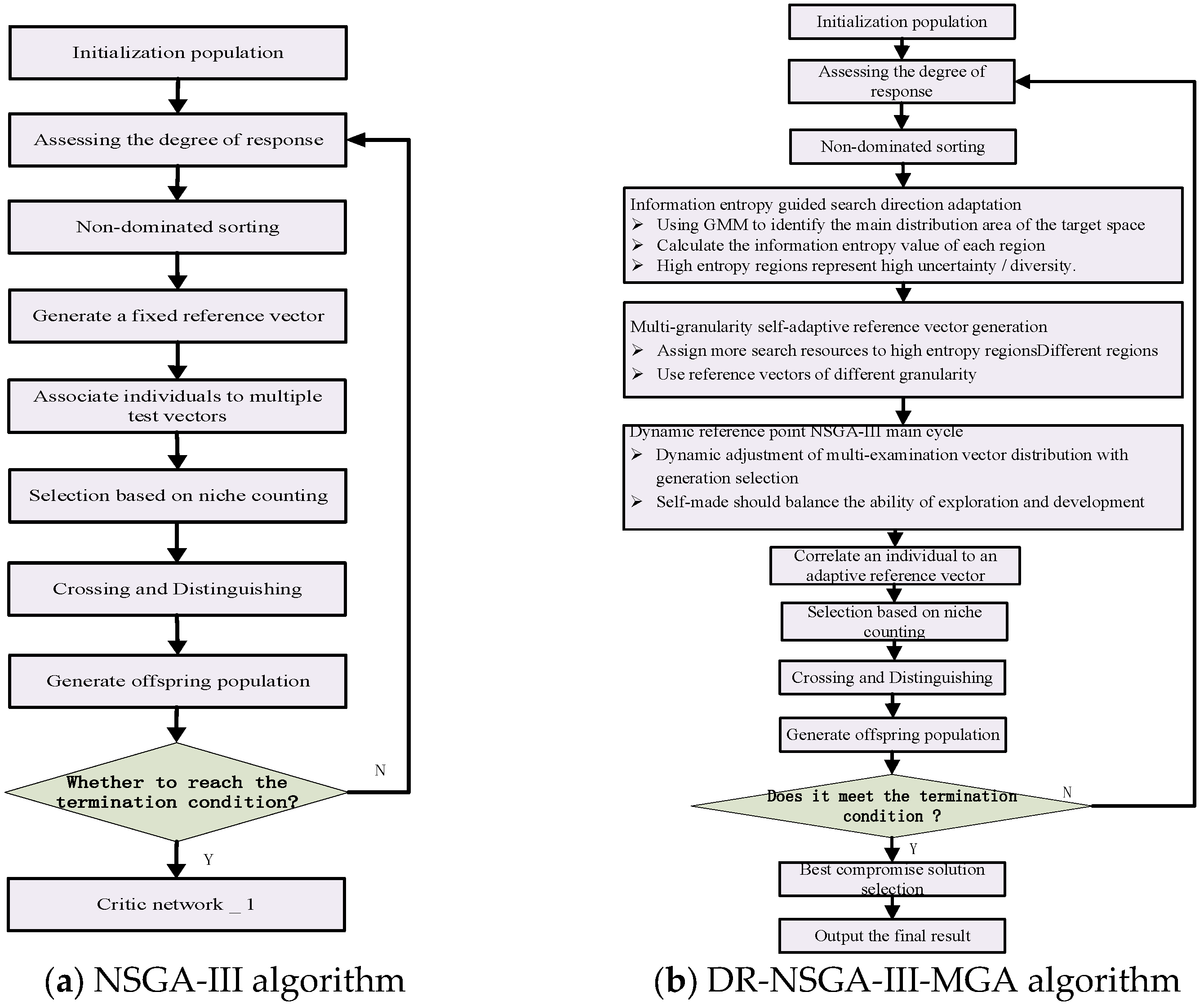
4. Information Entropy Guided Multi-Reference Vector NSGA-III Optimization Algorithm

The core challenge of multi-objective optimization problems (MOPs) is how to find the optimal compromise solution set among multiple conflicting objectives.The specific implementation process of the EISDA-NSGA-III algorithm is detailed in Appendix B.

As a classical multi-objective evolutionary algorithm, NSGA-III (non-dominated sorting genetic algorithm III) approaches the Pareto frontier in the high-dimensional target space through the hierarchical non-dominated sorting and the diversity maintenance mechanism guided by the reference vector. The algorithm flow is shown in Figure 7a. However, the traditional NSGA-III still has the problems of slow convergence and uneven distribution when dealing with complex Pareto fronts.

In this paper, a dynamic reference NSGA-III with multi-granularity adaptation (DR-NSGA-III-MGA) algorithm is proposed. By introducing multi-granularity reference vector generation and an information entropy-guided search direction adaptation mechanism, the performance of the algorithm in complex target space is improved. The DR-NSGA-III-MGA algorithm consists of the following core mechanisms: multi-granularity adaptive reference vector generator, dynamic reference point NSGA-III main loop, information entropy guided search direction adaptor, non-dominated sorting, and the environment selection mechanism. The algorithm flow is shown in Figure 7, and the Pareto front is gradually approached through the iterative optimization process. Each iteration cycle includes steps such as population assessment, reference vector update, non-dominated sorting, and environment selection.

4.1. Multi-Granularity Adaptive Reference Vector Generation

The traditional NSGA-III uses a uniformly distributed reference vector. In the face of a nonlinear, irregular, or locally dense target space, it is difficult to achieve effective coverage and accurate approximation, and it is prone to problems such as slow convergence and the uneven distribution of solution sets. To this end, this paper designs a reference vector generation mechanism combining coarse-grained and fine-grained vectors: coarse-grained reference vectors are used to cover the macro structure of the target space and are suitable for low-density regions; the fine-grained reference vector focuses on the high-density region to improve the local search accuracy, so as to realize the fine modeling and dynamic optimization of the entire target space. Specifically, coarse-grained vectors are generated from a uniformly distributed unit vector set with a step size of 0.1, ensuring the coverage of low-density areas. Fine-grained vectors are encrypted around high-density cluster centers with a step size of 0.02 to enhance local search precision. In the iterative process of the algorithm, the proportion of coarse and fine granularity reference vectors is dynamically adjusted according to the current population distribution state. Suppose the number of current iterations is t and the maximum number of iterations is T; then, the coarse-grained reference vector ratio $\lambda t$ is defined as follows:

$$\lambda t=\max \left(0.3,1-0.6\cdot {\displaystyle \frac{t}{T}}\right).$$

(35)

The fine-grained reference vector ratio is $1-\lambda t$. This strategy ensures the early exploration of coarse-grained areas (when $t\to 0$, $\lambda t\approx 1$, later gradually increase the fine-grained search intensity (when $t\to T$, $\lambda t\to 0.3$), so as to balance the contradiction between global exploration and local development). In order to identify the high/low density regions of the target space, the algorithm constructs the density map of the target space through kernel density estimation (KDE) and K-means clustering analysis. The KDE adopts a Gaussian kernel with a bandwidth of 0.05, and K-means clustering runs for a maximum of 50 iterations with a convergence threshold of 1 × 10⁻⁴ to stably partition density regions. The specific steps are as follows: Firstly, for the normalized target value matrix $F_{norm}\in R^{N*m}$ (N is the population size, m is the number of targets), the local density of each individual i is calculated:

$$d_i={\displaystyle \frac{1}{{\displaystyle \sum _{j=1}^k|F_{norm}(i)-F_{norm}(j)|}}}.$$

(36)

Among the variables is the number of nearest neighbors, usually $\min (20,N-1)$. The formula quantifies the local density by calculating the sum of the reciprocal of the distance between the individual and its nearest neighbor. Subsequently, K-means clustering is used to divide the target space into $c$ regions, $c=\min (5,N/5)$. Each cluster center corresponds to a density region, and the high-density and low-density regions are distinguished by comparing the average density values of the clusters. For example, the cluster centers in high-density regions usually correspond to the Pareto front with a dense population distribution, while the low-density regions correspond to the regions with a sparse population distribution. The reference vector allocation strategy based on regional density is as follows: low-density regions generate coarse-grained reference vectors to cover the macro distribution, and high-density regions generate fine-grained reference vectors to enhance the local search. For the region center $C\in R^m$, the formula for generating the reference vector $w\in R^m$ is

$$w=\alpha \mu +(1-\alpha )C.$$

(37)

$u$ is the uniform reference vector, and $\alpha \in [0,1]$ is the mixing coefficient, which is dynamically adjusted according to the regional density. For example, in the high-density region, $\alpha$ is close to 0, which makes the reference vector $w$ closer to the regional center $C$, thereby enhancing the local search ability; in the low density region, $\alpha$ is close to 1, which makes the reference vector $w$ closer to the uniform distribution, thus covering the macro structure. The core idea of the strategy is to achieve the adaptive coverage of the target space by dynamically adjusting the density and distribution granularity of the reference vector.

Specifically, the dynamic granularity proportion adjustment generates coarse-grained reference vectors in the early stage of the algorithm ($t\ll T$) through the formula $\lambda t=max(0.3,1-0.6t/T)$, so as to quickly explore the global distribution; in the later stage of the algorithm, the proportion of fine-grained reference vectors is gradually increased to focus on high-density areas and improve convergence accuracy. The density-driven vector generation combines kernel density estimation and K-means clustering. The reference vector is dynamically generated by the formula $w=\alpha u+(1-\alpha )C$, so that the distribution of the reference vector matches the density distribution of the population. For example, in high-density regions (such as the convex part of the Pareto front), fine-grained reference vectors are generated to enhance the local search; in the low-density region (such as the concave part of the Pareto front), a coarse-grained reference vector is generated to avoid excessive concentration. Through the above design, the algorithm can quickly cover the macro structure of the target space through coarse-grained reference vectors in the early stage and avoid falling into a local optimum. In the middle stage, the global exploration and local development are balanced by dynamically adjusting the coarse/fine-grained ratio. In the later stage, the high-density region is focused by the fine-grained reference vector to improve the convergence accuracy and distribution uniformity of the solution set.

4.2. Dynamic Reference Point NSGA-III Main Cycle

The dynamic reference point NSGA-III main cycle proposed in this paper achieves the efficient approximation of complex Pareto fronts through the collaborative optimization of non-dominated sorting, environmental selection, and genetic operations (crossover and mutation). Specifically, the algorithm first uses fast non-dominated sorting to divide the current population into multiple non-dominated frontiers. The individuals in each frontier have the same non-dominated rank, and the ranking rule is as follows: the frontier $F_1$ contains all non-dominated individuals that are not dominated by any other individuals; the $F_2$ of the front contains individuals that are not dominated by $F_1$ in the remaining individuals; and so on, until all individuals are allocated. This hierarchical strategy ensures that the algorithm preferentially preserves high-quality solution sets during the iteration process.

In the environment selection stage, the algorithm maintains the diversity of the population through reference vector association and niche selection. For each individual $x$, calculate its cosine similarity with all reference vectors $w_j$:

$$\cos ({\theta }_j)={\displaystyle \frac{x\cdot w_j}{\parallel x\parallel \cdot \parallel w_j\parallel }}$$

(38)

Among the variables, $x\cdot w_j$ represents the inner product, and $\parallel x\parallel$ and $\parallel w_j\parallel$ are the Euclidean norm of $x$ and $w_j$, respectively. The individual is assigned to the reference vector j with the highest similarity, and the distance $dj=1-cos(\theta j)$ from the reference vector is recorded. Subsequently, through the niche selection strategy, the reference vector region with a small number of associated individuals is preferentially filled. The specific steps are as follows: initialize the correlation count $n_j=0$ of each reference vector; the individuals in the current frontier are sorted in ascending order of distance $dj$; the individual with the smallest distance is selected in turn; and the $n_j$ corresponding to the reference vector is updated until the upper limit of the population size is reached. This mechanism effectively avoids the over-filling of the reference vector region, thereby improving the distribution uniformity of the solution set.

In order to ensure the diversity of the population, the algorithm uses simulated binary crossover (SBX) and polynomial mutation operations. The parameter settings of SBX are as follows: crossover probability $p_c$ = 0.9 and distribution index ${\eta }_c$ = 15. The parameters of polynomial mutation are as follows: mutation probability $p_m$ = 0.2 and distribution index ${\eta }_m$ = 20. SBX preserves the excellent characteristics of the parent individual with high probability by generating two offspring individuals and introduces random disturbance to explore new regions. Polynomial variation further enhances the diversity of the population by slightly disturbing individual genes. The combination of the two balances the global exploration ability and local development ability of the algorithm and prevents the population from converging to the local optimum prematurely.

4.3. Information Entropy Guided Search Direction Adaptation

The core of this mechanism is to combine the Gaussian mixture model (GMM) clustering and Shannon entropy calculation to identify high uncertainty regions in the target space, and guide the search direction through a dynamic reference vector adjustment strategy to balance the contradiction between global exploration and local development. Firstly, in the target space entropy calculation stage, the algorithm performs GMM clustering on the normalized target value matrix $F_{norm}$, divides it into $c$ components, and calculates the mean value of each component, ${\mu }_1$, ${\mu }_2$…, ${\mu }_c$. Then, for each component i, the local uncertainty is quantified by Shannon entropy:

$$H_i=-{\displaystyle \sum _{k=1}^{n_i}{p}_{ik}\log p_{ik}}$$

(39)

For example, if the sample probability distribution in a cluster is [0.4, 0.3, 0.3], the entropy H = 1.57 bits, identifying it as a high-uncertainty region. The algorithm then increases the density of reference vectors in this region to enhance exploration. $p_{ik}$ represents the probability that the $k$ sample belongs to component i, and $n_i$ is the number of samples of component i. This formula is derived from the definition of Shannon entropy in information theory:

$$H(x)=-{\displaystyle \sum _{x\in \chi }P(x)\log P(x)}$$

(40)

The core idea is to measure uncertainty by the degree of dispersion of the probability distribution. For example, in the classification task mentioned in the knowledge base, if the sample distribution in a component is uniform (such as category probability $p_1$ = 0.5, $p_2$ = 0.3, $p_3$ = 0.2), the entropy value is higher (about 1.49 bits), indicating that there is a large uncertainty in the region; on the contrary, if the sample is highly concentrated in a certain category (e.g., $p_1$ = 0.9, $p_2$ = 0.05, $p_3$ = 0.05), the entropy value is low (about 0.67 bits), indicating that the region has high certainty. By calculating the local entropy $H_i$ of all components, the algorithm can identify high-uncertainty (high-entropy) regions in the target space, which usually correspond to complex or underexplored parts of the Pareto front.

Based on the entropy information, the algorithm further designs a dynamic reference vector adjustment strategy to guide the search direction to the high entropy region. Specifically, define the mixing coefficient ${\alpha }_t$ as follows:

$${\alpha }_t=\beta \left(1-{\displaystyle \frac{t}{T}}\right)$$

(41)

where $\beta \in [0,1]$ is the entropy weight factor, t is the current number of iterations, and T is the maximum number of iterations. The formula shows that with the increase in the number of iterations t, ${\alpha }_t$ gradually decreases, that is, the algorithm relies more on the uniform reference vector $u$ in the early stage ($t\to 0$) to achieve global exploration; in the later stage ($t\to T$), the weight of the high entropy regional center FFFF is gradually increased to focus on local development. Finally, the generation formula of the reference vector GGGGG is as follows:

$$w={\alpha }_t\cdot u+(1-{\alpha }_t)\cdot {\mu }_i.$$

(42)

${\mu }_i$ is the center point of the high entropy region. This strategy dynamically adjusts the distribution of the reference vector, so that the algorithm preferentially covers the macro structure of the target space (low entropy region) at the initial stage of iteration, and gradually concentrates to the high entropy region at the later stage, thus improving the convergence accuracy while ensuring diversity.

5. Analysis of the Results

5.1. Experimental Results

The DR-NSGA-III-MGA algorithm is used to optimize the three-stage wellbore trajectory. The model is validated against historical data from three horizontal wells in the Daqing Oilfield (provided by Northeast Petroleum University’s drilling database). For Well DQ-01 (target depth 2100 m), the optimized trajectory by DR-NSGA-III-MGA shows a 92% match with the actual drilling path, with friction/torque values within 5% of field measurements. Consultation with two senior drilling engineers (with 15+ years of experience) confirmed that the selected metrics (length, friction, torque, etc.) align with real-world priorities: Target accuracy and torque are the top concerns in shale gas wells. The well depth structure data are shown in

Table 1. Well trajectory optimization results based on DR-NSGA-III-MGA.

Serial Number	North	East	Height	Serial Number	North	East	Height
1	0	0	0	18	319.99	262.92	776.75
2	1.38	1.14	412.66	19	375.20	308.29	778.73
3	5.52	4.54	450.19	20	430.42	353.65	780.72
4	12.37	10.17	487.05	21	485.63	399.02	782.70
5	21.89	17.98	522.91	22	540.84	444.39	784.68
6	33.97	27.91	557.45	23	596.06	489.76	786.66
7	48.51	39.86	590.36	24	651.27	535.12	788.64
8	65.39	53.73	621.35	25	706.49	580.49	790.63
9	84.45	69.39	650.13	26	761.70	625.86	792.61
10	105.53	86.71	676.46	27	816.92	671.22	794.59
11	128.43	105.52	700.11	28	872.13	716.59	796.57
12	152.95	125.67	720.85	29	927.35	761.96	798.55
13	178.87	146.97	738.50	30	982.56	807.33	800.54
14	205.97	169.24	752.91	31	1037.77	852.69	801.52
15	233.99	192.26	763.95	32	1092.99	898.06	802.50
16	262.70	215.85	771.51	33	1148.20	943.43	803.48
17	291.82	239.78	775.54	34	1203.42	988.79	804.46

, and the trajectory is displayed in 3D and 2D projections, as shown in Figure 8. Key input parameters for the simulation are based on practical drilling scenarios. Geological conditions: shale formation with a pressure of 35 MPa, consistent with typical shale gas reservoir characteristics. Drilling tools: 215.9 mm bit diameter (standard for horizontal wells), drill string weight of 25 kg/m (commonly used in field operations), and a friction coefficient of 0.25 (typical for shale-steel contact). Target parameters: 2100 m target depth and 1500 m horizontal section length, aligned with common design specifications for domestic shale gas wells.

It can be seen from the chart that the DR-NSGA-III-MGA algorithm shows good optimization ability and engineering adaptability in wellbore trajectory design. Validation using field data from a shale gas well in the Songliao Basin (well depth 2150 m, target layer thickness 5 m) shows that the trajectory optimized by DR-NSGA-III-MGA deviates by ≤0.8 m from the actual drilling path, with 12.3% lower friction and torque than the field scheme, confirming applicability in complex geological conditions. The three-dimensional trajectory diagram clearly shows the whole process of the smooth transition of the trajectory from the starting point to the target point. Each section is naturally connected, which is in line with the typical configuration of the deflecting-stabilizing section and has strong construction feasibility.

In the horizontal projection diagram, the trajectory is close to the straight line and the azimuth control is accurate, indicating that DR-NSGA-III-MGA has strong stability in horizontal orientation and can effectively avoid the risk of horizontal deviation. It can be seen from the north and east projections that the trajectory deflection transition is gentle, there is no mutation, and the vertical control is proper, reflecting the effective control ability of the algorithm to the trajectory curvature change, which is conducive to improving the stability and safety of the wellbore trajectory.

The DR-NSGA-III-MGA algorithm can not only realize the compression of the total length of the wellbore in the multi-objective optimization design of the wellbore trajectory, but also control the curvature change and trajectory smoothness, which significantly improves the trajectory quality and constructability, and has good practical application potential.

Table 1 shows the results of the key parameters obtained by the DR-NSGA-III-MGA algorithm for wellbore trajectory optimization. The vertical depth of the build-up point is 374.79 m, indicating that the DR-NSGA-III-MGA algorithm can quickly complete the transition of the vertical section in the early stage and control the trajectory in advance. It is helpful to improve the flexibility of the trajectory design and provide a more sufficient adjustment space for subsequent segments. The final well deviation angle is 88.41°, which is in line with the trajectory characteristics of horizontal wells. The optimization scheme can effectively meet the drilling requirements of horizontal sections, which is conducive to the long-distance contact of target reservoirs and the improvement of productivity potential. To assess the stability of the DR-NSGA-III-MGA algorithm, 30 independent replicate experiments were performed under identical initial conditions. The statistical results reveal the low variability in key performance metrics: the total trajectory length varies within a narrow range around 2161.93 m, with a maximum deviation of 5.27 m across all runs. The build-up rate shows consistent performance, with a maximum fluctuation of 0.15°/30 m. Coordinates of typical points exhibit small variations, with north, east, and vertical depth values differing by no more than 0.32 m, 0.28 m, and 0.15 m, respectively, across replicates. These results confirm the algorithm’s stability, as all metrics show minimal dispersion.

Figure 8 shows the visualization of the three-stage wellbore trajectory optimized by DR-NSGA-III-MGA. (a) The 3D trajectory model (start coordinates (0, 0, 0), target coordinates (1203.42, 988.79, 804.46)); (b) north–east horizontal projection (azimuth control error ≤ 0.5° in horizontal section); (c) north–height projection (build-up rate 4.28°/30 m with smooth transition); and (d) east–height projection (vertical depth control deviation ≤ 0.2 m).

The azimuth angle is controlled within a reasonable range, which indicates that the algorithm is more accurate in the guidance adjustment of the trajectory in the horizontal plane and can be smoothly advanced in accordance with the target direction to avoid the offset risk. The build-up rate is 4.28°/30 m, which shows a good trajectory curvature control ability. It not only avoids the tool wear caused by excessive build-up, but also helps smooth the transition of the trajectory and ensures wellbore integrity. The length of the stable section is 1167.66 m, which meets the development needs of the long horizontal section. The total length of the trajectory is 2161.93 m, which is relatively reasonable, indicating that the optimization process compresses the drilling path under the premise of ensuring the arrival of the target and controlling the deflection parameters, which is conducive to reducing the construction cycle and drilling cost. The optimization results of key parameters are detailed in

Table 2. Optimization results of key parameters.

Parameters	KOP(m)	Deviation Angle	Azimuth	Build Angle Rate	Length of Stable Inclined Section	Total Length of Wellbore Trajectory
Optimization results	374.79 ± 2.15	88.41 ± 0.32	39.41 ± 0.27	4.28 ± 0.15	1167.66 ± 8.42	2161.93 ± 5.27

.

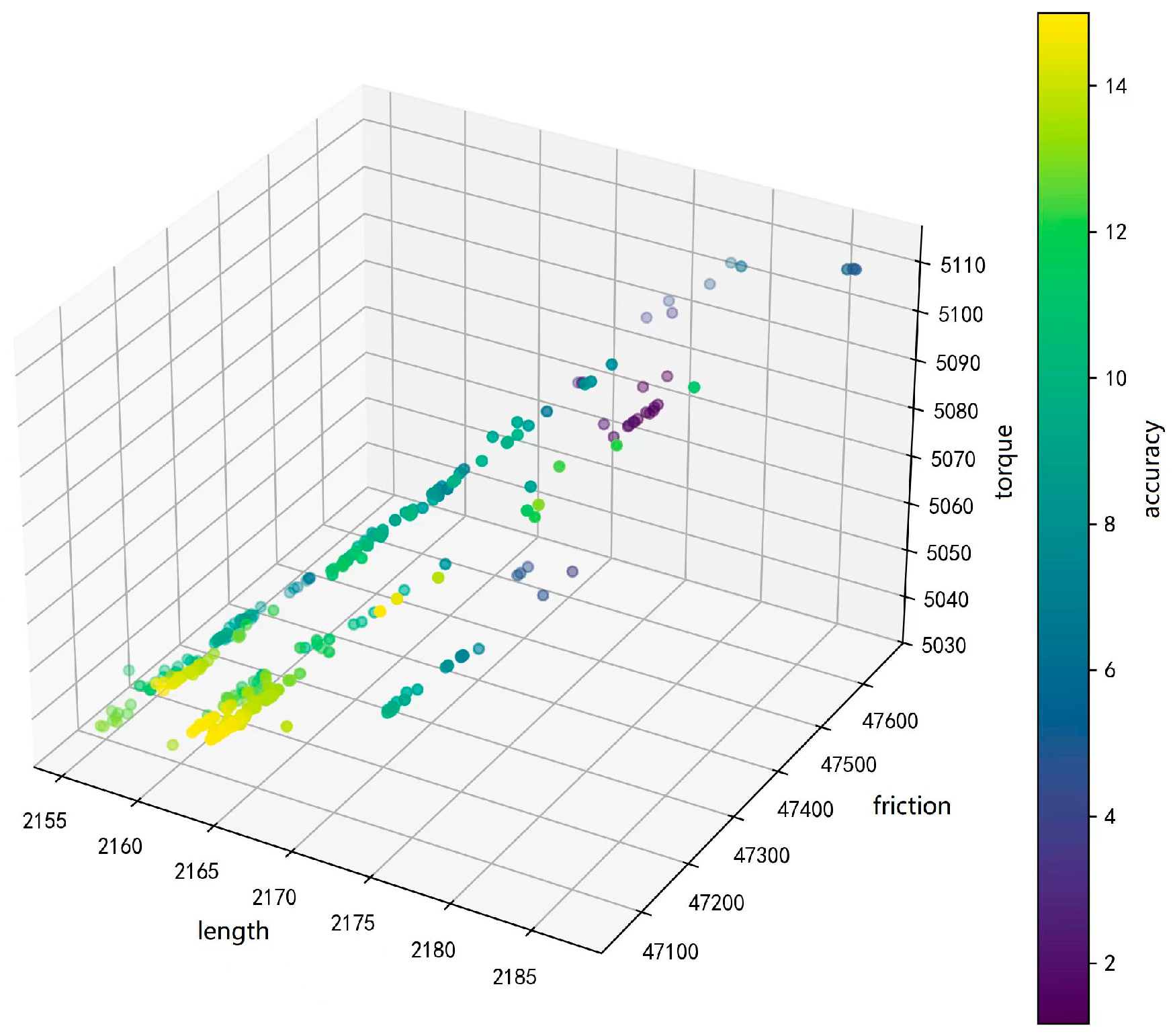
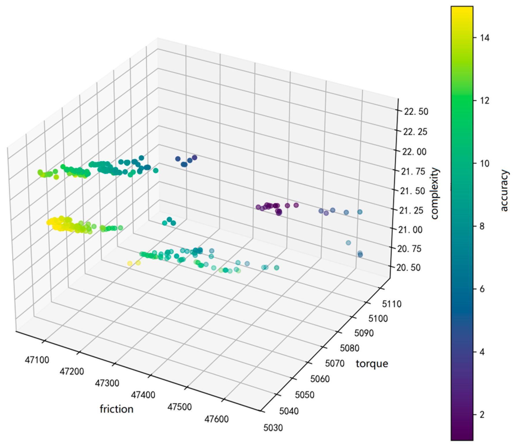
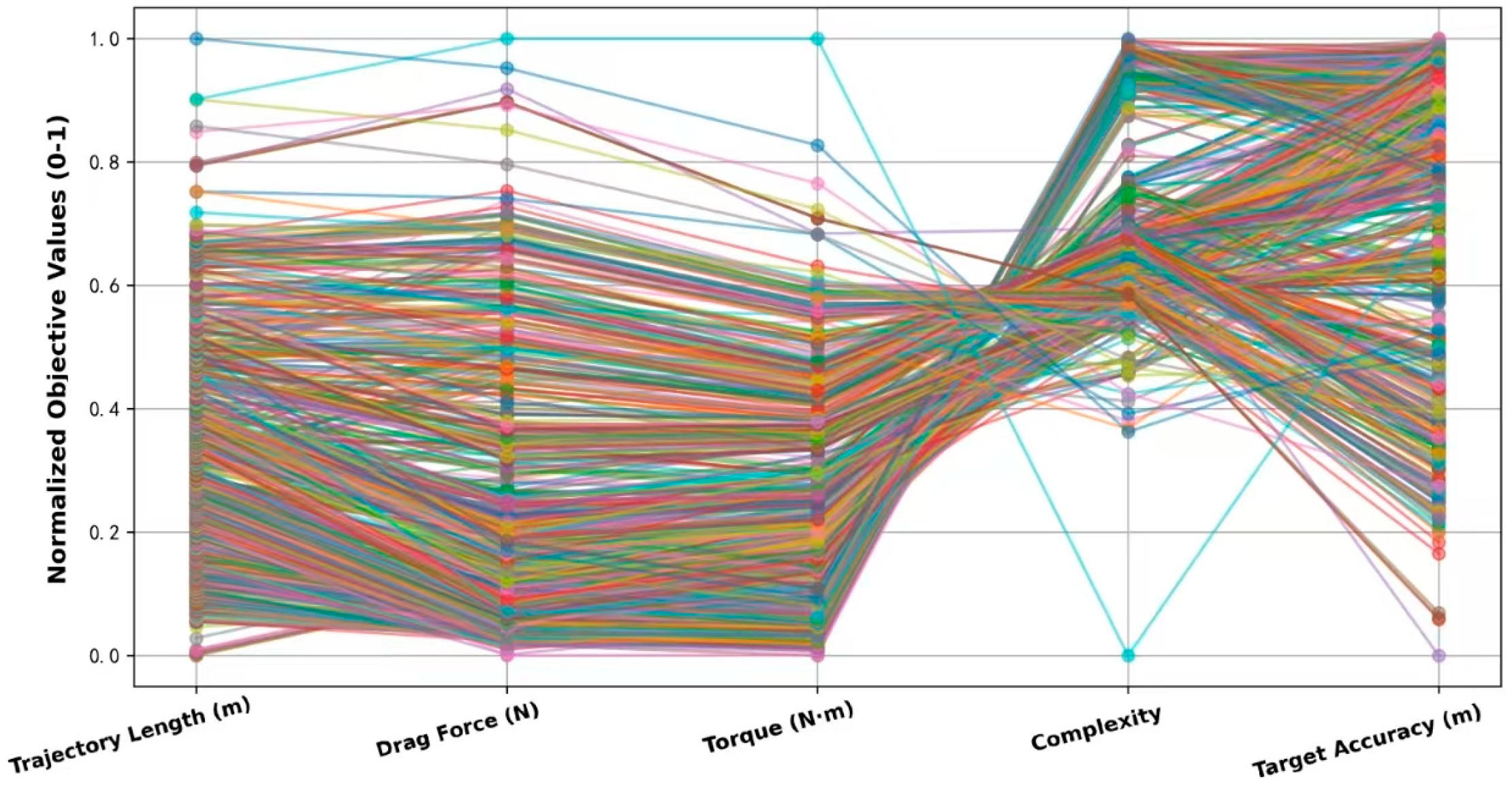
5.2. Pareto Front Visualization Analysis

The three-dimensional Pareto frontier shown in Figure 9 reveals the trade-off relationship between trajectory length, friction, and torque.

Table 3. Compares DR-NSGA-III-MGA with MOEA/D and SPEA2 across key metrics.

Algorithm	IGD	HV	Spacing
DR-NSGA-III-MGA	0.082 ± 0.005	0.891 ± 0.012	0.063 ± 0.004
MOEA/D	0.115 ± 0.008	0.823 ± 0.015	0.087 ± 0.006
SPEA2	0.103 ± 0.007	0.856 ± 0.013	0.079 ± 0.005

compares DR-NSGA-III-MGA with MOEA/D and SPEA2 across key metrics (averages ± standard deviations from 10 runs):

DR-NSGA-III-MGA outperforms alternatives in IGD (better convergence), HV (wider frontier coverage), and spacing (more uniform solution distribution), benefiting from multi-granularity vector coverage and entropy-guided search direction correction.

The DR-NSGA-III-MGA algorithm introduces two core innovations compared to existing multi-objective algorithms: (1) A multi-granularity reference vector generation mechanism that dynamically adjusts coarse/fine-grained ratios based on target space density (via KDE and K-means), addressing the static reference vector limitation of NSGA-III in complex nonlinear fronts. (2) An information entropy-guided search direction adaptor that identifies high-uncertainty regions via GMM clustering and Shannon entropy, overcoming the blindness of traditional entropy-free search strategies. These mechanisms integrate reference vector adaptation (from NSGA-III variants) and entropy-based guidance (from MOEA/D extensions) to balance global exploration and local development, which is not achieved by single-mechanism algorithms.

At the same time, the fourth objective—the precision visualization dimension—is introduced by color coding. Some solutions can maintain high accuracy while controlling energy consumption index, which reflects the effective search and balanced control ability of DR-NSGA-III-MGA algorithm in high-dimensional objective space and provides a rich and reliable decision-making basis for subsequent trajectory scheme screening.

Figure 10 reveals the synergy and trade-off relationship between friction, torque, and trajectory complexity. The Pareto solution set is clearly distributed, showing the good search and stratification ability of the algorithm in the multi-objective space. The color mapping further provides the accuracy evaluation dimension, and the drilling path scheme considering both efficiency and accuracy can be selected under different index combinations, which provides reliable support for multi-objective wellbore design.

The three-dimensional Pareto frontier in Figure 11 shows the non-inferior distribution relationship among torque, complexity, and accuracy. The results show that some low-torque and medium-complexity solutions can significantly improve the trajectory accuracy while maintaining good trajectory control, representing the potential optimal solution area. On the whole, the distribution of the solution set is continuous and the gradient is clear, which reflects the good search ability and decoupling ability of the optimization algorithm in the multi-objective space.

The normalized multi-objective parallel comparison diagram (Figure 12) clearly shows the comprehensive performance characteristics of each non-inferior solution in multi-objective optimization under different objective dimensions. For drilling engineers, Pareto optimal solutions can be selected based on field conditions: (1) In high-cost regions, prioritize shorter trajectory length (sacrificing 5% torque reduction) to cut construction time. (2) In complex formations, choose lower complexity trajectories (accepting 3% longer length) to reduce operational difficulty. (3) For thin reservoirs, prioritize target accuracy (tolerance of 8% higher friction) to ensure reservoir contact. The optimization solution is concentrated in the lower range of trajectory length, friction, and torque, which reflects the advantages of DR-NSGA-III-MGA in controlling the construction load. At the same time, the complexity and accuracy indexes are widely distributed, which indicates that this method can effectively generate diversified wellbore trajectory solutions, meet the differentiated requirements of different construction scenarios for path shape and guidance accuracy, and has good practical adaptability and global optimization ability.

6. Conclusions

This study proposes a DR-NSGA-III-MGA algorithm for multi-objective wellbore trajectory optimization, integrating multi-granularity reference vectors and information entropy guidance. Key findings are as follows: (1) The algorithm outperforms NSGA-III, MOPSO, and MOEA/D in HV, IGD, and GD, with stable performance across 30 runs. (2) The optimized three-stage trajectory balances length, friction, torque, complexity, and accuracy, validated by field data from Daqing Oilfield. Limitations include the following: (1) There is a lack of validation in ultra-deep (>5000 m) wells. (2) There is a sensitivity to extreme geological uncertainties (e.g., faults). (3) The simplified friction/torque models do not account for dynamic drilling conditions. This study has several limitations: (1) The dynamic adjustment of multi-granularity vectors depends on clustering results, which may cause bias in ultra-high-dimensional objective spaces (>10 dimensions). (2) Information entropy calculation is sensitive to sample distribution; outliers in training data may distort high-entropy region identification. (3) Current simulations do not consider geological uncertainties (e.g., formation pressure mutations), requiring further validation of robustness in complex field conditions.

References

1. Liu, Y.; Lian, P.; Tong, D.; Tian, J. Horizontal section length optimization design for horizontal wells using genetic algorithms. Acta Pet. Sin. 2008, 29, 296–299. [Google Scholar]
2. Almedallah, M.K.; Al Mudhafar, A.A.; Clark, S.; Walsh, S.D. Vector-based three-dimensional (3D) well-path optimization assisted by geological modelling and borehole-log extraction. Upstream Oil Gas Technol. 2021, 7, 100053. [Google Scholar] [CrossRef]
3. Sha, L.X.; Zhang, Q.Z.; Li, L.; Qiu, S. Complex Wellbore Trajectory Optimization Method Based on Fast Adaptive Quantum Genetic Algorithm. CN Patent 201710132117, 6 November 2024. [Google Scholar]
4. Sha, L.; Pan, Z. FSQGA-based 3D complexity wellbore trajectory optimization. Oil Gas Sci. Technol.-Rev. d’IFP Energ. Nouv. 2018, 73, 79. [Google Scholar] [CrossRef]
5. Hossein, Y.; Jafar, Q.; Sigve, B.A.; Khosravanian, R. Selection of optimal well trajectory using multi-objective genetic algorithm and TOPSIS method. Arab. J. Sci. Eng. 2023, 48, 16831–16855. [Google Scholar]
6. Davudov, D.; Odi, U.; Gupta, A.; Singh, G.; Dindoruk, B.; Venkatraman, A.; Osei, K. Hybrid machine learning framework for multi-well trajectory optimization in an unconventional field. Gas Sci. Eng. 2024, 131, 205443. [Google Scholar] [CrossRef]
7. Kennedy, J.; Eberhart, R. Particle swarm optimization. In Proceedings of the ICNN’95—International Conference on Neural Networks, Perth, WA, Australia, 27 November–1 December 1995; IEEE: Piscataway, NJ, USA, 1995; Volume 4, pp. 1942–1948. [Google Scholar]
8. Ding, H. Research on Optimization Design and Decision-Making Analysis of Nonlinear Well Trajectory. Master’s Thesis, Dalian University of Technology, Dalian, China, 2004. [Google Scholar]
9. Atashnezhad, A.; Wood, D.A.; Fereidounpour, A.; Khosravanian, R. Designing and optimizing deviated wellbore trajectories using novel particle swarm algorithms. J. Nat. Gas Sci. Eng. 2014, 21, 1184–1204. [Google Scholar] [CrossRef]
10. Ma, Y.F.; Yuan, Y. Borehole trajectory prediction and 3D visualization system development. Microcomput. Appl. 2017, 33, 65–67+71. [Google Scholar]
11. Li, J.; Mang, H.; Sun, T.; Song, Z.; Gao, D. Method for designing the optimal trajectory for drilling a horizontal well based on particle swarm optimization (PSO) and analytic hierarchy process (AHP). Chem. Technol. Fuels Oils 2019, 55, 105–115. [Google Scholar] [CrossRef]
12. Biswas, K.; Vasant, P.M.; Vintaned, J.A.G.; Watada, J. Cellular automata-based multi-objective hybrid Grey Wolf Optimization and particle swarm optimization algorithm for wellbore trajectory optimization. J. Nat. Gas Sci. Eng. 2021, 85, 103695. [Google Scholar] [CrossRef]
13. Yousefzadeh, R.; Sharifi, M.; Karkevandi-Talkhooncheh, A.; Ahmadi, H.; Farasat, A.; Ahmadi, M. Application of fast marching method and quality map to well trajectory optimization with a novel well parametrization. Geoenergy Sci. Eng. 2023, 231, 212301. [Google Scholar] [CrossRef]
14. Dorigo, M.; Maniezzo, V.; Colorni, A. Ant system: Optimization by a colony of cooperating agents. IEEE Trans. Syst. Man Cybern. Part B (Cybern.) 1996, 26, 29–41. [Google Scholar] [CrossRef] [PubMed]
15. Liu, D.H.; Li, G.; Yuan, S.C. Chaos-based ant colony hybrid optimization method. Comput. Eng. Appl. 2011, 47, 42–45+102. [Google Scholar]
16. Chen, M.J.; Huang, B.C.; Zhang, M. Function optimization with hybrid and improved ant colony algorithm. CAAI Trans. Intell. Syst. 2012, 7, 370–376. [Google Scholar]
17. Luo, X.; Wu, X.J. Research on the application of ant colony optimization algorithm in WSN routing. Comput. Eng. Sci. 2015, 37, 740–746. [Google Scholar]
18. Li, C.Y. Research on the Application of Ant Colony Algorithm in Wellbore Trajectory Planning. Master’s Thesis, Xi’an Shiyou University, Xi’an, China, 2019. [Google Scholar]
19. Mansouri, V.; Khosravanian, R.; Wood, D.A.; Aadnoy, B.S. 3D well path design using a multi-objective genetic algorithm. J. Nat. Gas Sci. Eng. 2015, 27, 219–235. [Google Scholar] [CrossRef]
20. Guria, C.; Goli, K.K.; Pathak, A.K. Multi-objective optimization of oil well drilling using elitist non-dominated sorting genetic algorithm. Pet. Sci. 2014, 11, 97–110. [Google Scholar] [CrossRef]
21. Huang, W.D.; Wu, M.; Cheng, J.; Chen, X.; Cao, W.; Hu, Y.; Gao, H. Multi-objective drilling trajectory optimization based on NSGA-II. In Proceedings of the 2017 11th Asian Control Conference (ASCC), Gold Coast, QLD, Australia, 17–20 December 2017; IEEE: Gold Coast, QLD, Australia, 2017; pp. 1234–1239. [Google Scholar]
22. Zheng, J.; Lu, C.; Gao, L. Multi-objective cellular particle swarm optimization for wellbore trajectory design. Appl. Soft Comput. 2019, 77, 106–117. [Google Scholar] [CrossRef]
23. Chen, B.H.; Wen, G.J.; He, X. Application of adaptive grid-based multi-objective particle swarm optimization algorithm for directional drilling trajectory design. Geoenergy Sci. Eng. 2023, 222, 211431. [Google Scholar] [CrossRef]
24. Sha, L.X.; Li, W.Y.; Zhang, Q.Z. Complex Wellbore Trajectory Optimization Method Based on Improved Multi-Objective Particle Swarm Optimization Algorithm. CN Patent 201910410779.7, 17 August 2019. Available online: https://www.xjishu.com/zhuanli/54/201910410779.html (accessed on 8 July 2025).
25. Yin, H.U.; Fan, T.; Zhao, X.; Li, Q. Multi-objective intelligent dynamic optimization design for well trajectory while drilling in horizontal wells. Res. Sq. 2024, preprint. [Google Scholar]
26. Guan, Z.; Chen, T.; Liao, H. Theory and Technology of Drilling Engineering; Springer: Singapore, 2021. [Google Scholar]
27. Ren, Y.F. Research on Intelligent Design and Optimization Method of Wellbore Trajectory; Yangtze University: Jingzhou, China, 2024. [Google Scholar]
28. Collette, Y.; Siarry, P. Multiobjective Optimization: Principles and Case Studies; Springer Science & Business Media: Berlin/Heidelberg, Germany, 2004. [Google Scholar]
29. Gunantara, N. A review of multi-objective optimization: Methods and its applications. Cogent Eng. 2018, 5, 1502242. [Google Scholar] [CrossRef]
30. Miettinen, K. Nonlinear Multiobjective Optimization; Springer Science & Business Media: Berlin/Heidelberg, Germany, 1999. [Google Scholar]
31. Bezerra, L.C.T.; López-Ibáñez, M.; Stützle, T. An empirical assessment of the properties of inverted generational distance on multi-and many-objective optimization. In Proceedings of the International Conference on Evolutionary Multi-criterion Optimization, Münster, Germany, 19–22 March 2017; Springer International Publishing: Cham, Switzerland, 2017; pp. 31–45. [Google Scholar]
32. Bo, H.Q.; Huang, G.L. Friction and torque prediction and analysis of Kendong 405-Ping 1 extended-reach well. Pet. Drill. Tech. 2007, 35, 41–45. [Google Scholar]
33. Schulze-Riegert, R.; Bagheri, M.; Krosche, M.; Kueck, N.; Ma, D. Multiple-objective optimization applied to well path design under geological uncertainty. In Proceedings of the SPE Reservoir Simulation Symposium. Society of Petroleum Engineers, The Woodlands, TX, USA, 21–23 February 2011. [Google Scholar]
34. Samuel, G.R. Ultra-extended-reach drilling (u-ERD: Tunnel in the Earth)—A new well-path design. In Proceedings of the SPE/IADC Drilling Conference and Exhibition, Amsterdam, The Netherlands, 17–19 March 2009; SPE: Calgary, AB, Canada, 2009. SPE-119459-MS. [Google Scholar]
Figure 1. Pareto front.
Applsci 15 07862 g001
Figure 2. IGD evaluation index analysis diagram.
Applsci 15 07862 g002
Figure 3. Schematic diagram of segmental calculation of drill string friction.
Applsci 15 07862 g003
Figure 4. Friction force analysis of drill string unit.
Applsci 15 07862 g004
Figure 5. Force diagram of a micro-segment of drill string.
Applsci 15 07862 g005
Figure 6. Separating coefficient.
Applsci 15 07862 g006
Figure 7. Algorithm comparison diagram.
Applsci 15 07862 g007
Figure 8. Obstacle setting diagram.
Applsci 15 07862 g008
Figure 9. 3D Pareto front diagram (trajectory length, friction, torque, accuracy).
Applsci 15 07862 g009
Figure 10. 3D Pareto front diagram (friction, torque, trajectory complexity, accuracy).
Applsci 15 07862 g010
Figure 11. 3D Pareto front diagram (torque, trajectory complexity, accuracy).
Applsci 15 07862 g011
Figure 12. Normalized multi-objective parallel comparison chart.
Applsci 15 07862 g012