Optimizing Contrastive Learning with Semi-Online Triplet Mining

Abstract

Contrastive learning is a machine learning technique in which models learn by contrasting similar and dissimilar data points. Its goal is to learn a representation of data in such a way that similar instances are close together in the representation space, while dissimilar instances are far apart. Our industrial use case focuses on a special case of contrastive learning called triplet learning. Building triplets with adequate difficulty is crucial to effective training convergence in such a setup. By combining online and offline mining techniques, we propose a method of mining hard triplets that is both performant and memory-inexpensive. Our experiments demonstrate that the method leads to improved identity pairing (which is the specific case of clustering) both on a real-life industry shoe dataset and on a generated benchmark one.

1. Introduction

This article presents a method of optimizing contrastive learning by controlling the ordering of examples in a dataset which we devised while solving a real-life industry problem. Our findings can be applied to most of the contrastive learning methods available, although this article focuses on triplet learning.

Contrastive learning is a technique that creates a model that seeks to distinguish between the “same” and “different” examples. It has been used to solve classification-like problems with a variable number of classes: verification, similarity computation, or clustering problems [1]. In the process, an embedding transformation is learned to transform original data points into a compact vector representation (typically hundreds or thousands of dimensions) with the desired properties. Such a process often entails the “same” examples ending close to each other in the embedding space and “different” ones ending far away from each other.

Our real-life industry problem is similar, as we must identify pairs in a large set of second-hand shoes for our client, VIVE Textile Recycling. A shoe is hung on a dedicated hanger and travels through the firm’s facility via an automated overhead transport (AOT) system. It gets photographed from three angles inside one of two photobooths during this process.

The solution we develop together with VIVE must achieve the highest possible pairing accuracy solely due to the scale of the operation. The processing of over two million shoes per month makes even a small fraction of the errors worth correcting, as they can easily amount to considerable losses. The shoe stream is large and diverse, as it comprises used footwear collected from across Europe. This volume and variance render the model’s training even more difficult, as it is challenging for similar-but-different pairs to be found, retrieved, and used in contrastive learning.

Our previous work [2] describes how we used triplet learning with a three-image-input VGG-inspired convolutional deep neural network to achieve high pairing accuracy. We opted to name shoes that belong to the same pair as “same” and shoes that do not as “different”. This decision has the drawback of making the embedding transformation laterality agnostic, which means that our main network cannot differentiate left shoes from right ones. Triplet loss [2] pulls the embeddings of anchor A (e.g., a left shoe) and positive example P (e.g., a right shoe) closer together, while pushing the embedding of negative example N (a nonmatching shoe) away. In other words, we force the network to transform left- and right-shoe images into the same region of the embedding space. Laterality is handled separately by a dedicated network, a simple binary image classifier. Later, we use this information to avoid pairing two left shoes together.

In classical machine learning problems, such as classification, examples are independent. Triplet learning is different because a single input to the network comprises three distinct dataset examples, one reference (anchor) example, one positive example (being “the same” as the anchor), and one negative example (“different” from the anchor). Therefore, an implicit relation between different examples in the dataset exists. Due to this relation, alongside the properties of triplet learning and triplet loss itself, training in this regime might be more challenging than classical problems like classification. We experienced this problem during the training of our pairing network. As the training progressed, relatively soon into the process, triplet loss started to become zero on progressively more batches. The zeroing of the loss function meant that there were no gradient and no updates to the model parameters, despite quite many errors continuing to exist on the test dataset. This happens because randomly selected triplets tend to be relatively easy, which means that even simple (or untrained) models’ embeddings already satisfy the triplet loss equation. We may consider a triplet that comprises an anchor and positive examples: a red pair of chucks and a green wellington as a negative example. They can be distinguished easily by sight. Such triplets do not force the network to focus on fine details but enable it to concentrate on much less complicated features, like overall color. This suggests the importance of hard triplets in the process. This article discusses this in detail in its Section 2 and Section 6.

Section 2 also reviews the literature in this area. The Section 3 describes the proposed method with some background knowledge and notation. The Section 5 presents the experiments we conducted along with their results.

2. Related Work

A growing number of examples exist of the use of AI-based methods in textile recycling—or, more broadly, the apparel industry [3]. Many of them are, at base, examples of material classification with the support of machine learning. Such classification is often performed using spectral imagery, which can exploit the fact that different electromagnetic wavelengths interact with particular materials in particular ways [4,5,6]. Other applications in the field include clothing classification by garment type (e.g., jeans, shirts, and jackets) [7] and the color classification of wool fabrics [8]. In the footwear domain, prior research focuses on brand identification [9] and shoe style classification [10].

Surprisingly little research has been produced on the shoe pairing process. Our previous study [2] established the base model that we continue to use in this work. We use a convolutional neural network [11,12] as an embedding generator. We tested many modern architectures, including CLIP [13], dense networks [14], EfficientNet [15], Inception [16], and ResNet [17]. We settled for a relatively old VGG16 [18] network, which yielded the best tradeoff between pairing accuracy and computational overhead for our application. We define pairing accuracy as in Equation (1). It remains the master metric of performance throughout the research process because it is crucial in business. It gets maximized indirectly by the minimization of triplet loss (2) using SGD methods.

$$pairingaccuracy\left(S\right)={\displaystyle \frac{\left|shoescorrectlyassignedmatchingshoe\right|+\left|shoescorrectlyleftunpaired\right|}{\left|allshoesinshoesetS\right|}}$$

(1)

Three input images are processed with independent VGG16 networks (stripped of the dense layers); global average pooling [19] is then performed on each branch before they get concatenated and processed with final dense layers. We use transfer learning [20] for initializing convolutional features from ImageNet pretraining. The architecture of our network is described in our previous work in great detail [2].

To train effective embeddings, we use the triplet loss function as defined in [1], which is given by Equation (2). T is a set of triplets in the form $(x^a,x^p,x^n)$ (anchor, positive, and negative) of size N. E is our neural network model that creates the embeddings, while d is a metric; we use Euclidean distance as in [1]. m is the parameter responsible for the separation margin. We later use $D=\{\{x_1^1,x_1^2\},\{x_2^1,x_2^2\},\{x_3^1,x_3^2\},...\}$ to denote a dataset. The subscript denotes the identity of an example, and the superscript describes the order within an identity.

$$L\left(T\right)=\sum _{i=1}^{N}max(0,d(E\left(x_i^a\right),E\left(x_i^p\right))-d(E\left(x_i^a\right),E\left(x_i^n\right))+m)$$

(2)

As the authors of [1] suggest, searching for hard or at least semi-hard examples is helpful because easy examples satisfy the triplet inequality early in the training process. Hard triplets are those for which the model (at some point in training) places the embedding of a negative example closer to the anchor than a positive one. In a semi-hard triplet, the negative embedding distance from the anchor is greater than the positives but less than the margin. The authors also distinguish two methods of searching. The first is offline mining, which depends on preparing the triplets every N training steps with the current state of the embedding network on a subset of data. The disadvantage of the offline approach is that the triplets used in training result from an old, now nonexistent model (as its parameters have changed). This can make them suboptimal for learning. Online mining searches for hard triplets only within mini-batches, which results in a smaller population of examples being considered for hard triplets simultaneously, with the possibility of valuable ones being missed. The authors focus on the online approach, as they could afford mini-batches of a few thousand examples.

3. Method

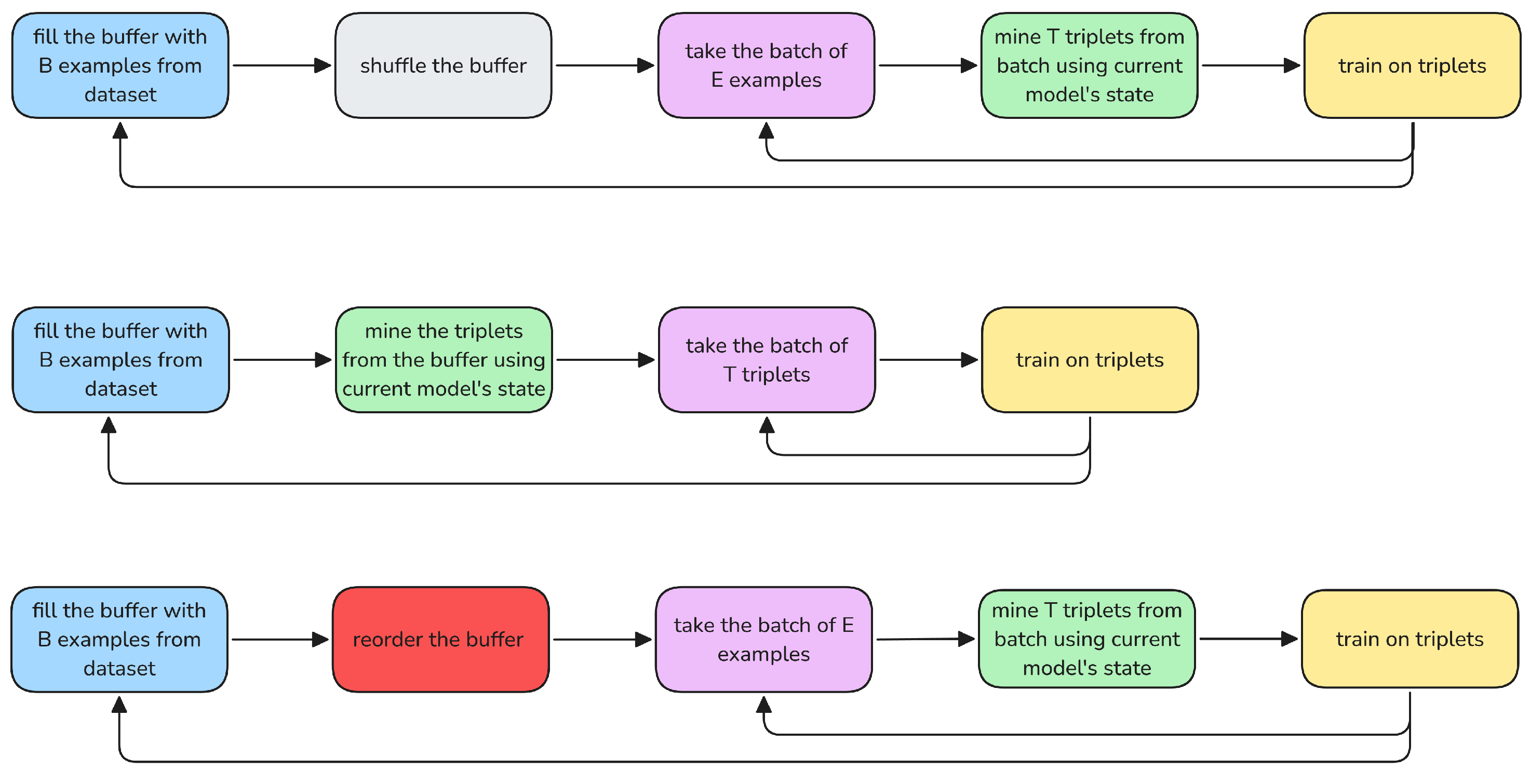
Our method strives to maintain the best of both worlds while limiting the adversarial effects. The name “semi-online” stems from the combination of online, batch-level search for the best triplets with offline, periodic dataset reordering. High-level comparison of these is shown on Figure 1. To preserve the principle of using embeddings inferred by the latest state of the trained model, the online triplet mining stage remains unchanged. The proposed novelty lies in the addition of an extra step before batching: the (offline) reordering of the dataset in a manner that favors similar examples (but with different identities) being closer together, thus increasing the probability of them getting into the same mini-batch. The rationale is that such a regime creates better-performing models by enabling online triplet mining to find more (semi-)hard negative examples. One way of formalizing this involves seeking batch $B=\{x_1^1,x_1^2,x_2^1,x_2^2,x_3^1,x_3^2,...\}$ with minimal ${\sum }_{1\le i<j\le n}d(E\left(x_i^1\right),E\left(x_j^1\right)$. Whether this is the optimal formulation of that idea remains unknown. It is possible that a batch that has a single but very hard example for every identity (i.e., ${\sum }_{i}d(E\left(x_i^1\right),E\left({arg\; min}_{x_j}d(E\left(x_i^1\right),E\left(x_j^1\right))\right))$) would be better for training the embedding network (in terms of pairing accuracy) than a batch in which, for every identity, every other identity creates a moderately hard triplet. The relation between batch properties and pairing accuracy seems intractable; therefore, no single best criterion on the batch itself can be formed.

Figure 2 presents a visual representation of the process. This method is akin to using a larger mini-batch size without needing more memory on the GPU or accelerator. It differs from the gradient accumulation technique [21], however, because the gradient is still calculated based on a smaller mini-batch. Only the triplet mining aspect is upgraded.

In our method, similarly to offline triplet mining, the frequency of the performance of the extra work and the number of data searched can be selected arbitrarily. Regarding frequency, reordering examples too frequently leads to considerable computational overhead but can also cause the order to align better with the current state of the model (less outdated). Using high frequencies is not as crucial as it is in offline mining because the subsequent online mining step will use the current model to calculate the most recent embeddings. The fraction of the dataset being searched and ordered simultaneously is also a tradeoff: using the small buffer of identities will not improve the performance and will ultimately collapse into simple online mining (no meaningful reordering occurs when the buffer size is equal to the batch size). Although reordering the whole dataset entails the heaviest computational overhead (the complexity of this process is higher than linear), it is also capable of finding and exaggerating errors in the dataset. We discovered the reordering of the whole dataset once every five epochs to be a reasonable tradeoff.

A running buffer of carefully ordered examples is maintained to enable online triplet mining to work best. In our dataset, examples (shoes) that have the same identity (coming from the same pair) always go together. Therefore, reordering the dataset means changing the order of the identities (pairs). The method described below operates on a set of points in n-dimensional space and returns an ordered list of these points. The structure of the dataset is more complicated, as it comprises photos grouped into identities. As examples within an identity are (by definition) similar, we simply select the first example from every identity to be its representative. Then, after the processing of the photographs using an embedding network, the photographs become points, and the proposed point-reordering method is applied, so that the identity order is established. As a final step, the initial dataset is reordered to match the newly calculated order.

Considering that the embeddings are points located on a multi-dimensional unit sphere, ordering them is a considerable task. There is no obvious way to do it. Even the principle of “similar identities should go close to each other” can be formalized in countless ways. The tasks has much in common with the traveling salesman problem (TSP) [22]—although differences can be observed. First, in the TSP, the path forms a loop, which is not required in our scenario. Second, the TSP would penalize jumping between very remote clusters in suboptimal order; in our problem, this is unimportant. When presented with three groups of shoes—chucks, wellingtons, and derbys—the order of the groups is irrelevant as long as similar chucks, for example, are close to each other. The TSP, on the other hand, would focus on optimizing the path between such remote clusters, as the distance between them is large and would affect the length of the total path markedly. This observation hints that local similarity should be given more attention than global similarity in the ordering problem. This second property, “local proximity first”, is the reason why manifold learning techniques like t-SNE [23] and UMAP [24] were dropped: finely controlling this property within them would be challenging. To fulfill these requirements, we have devised a two-step approach.

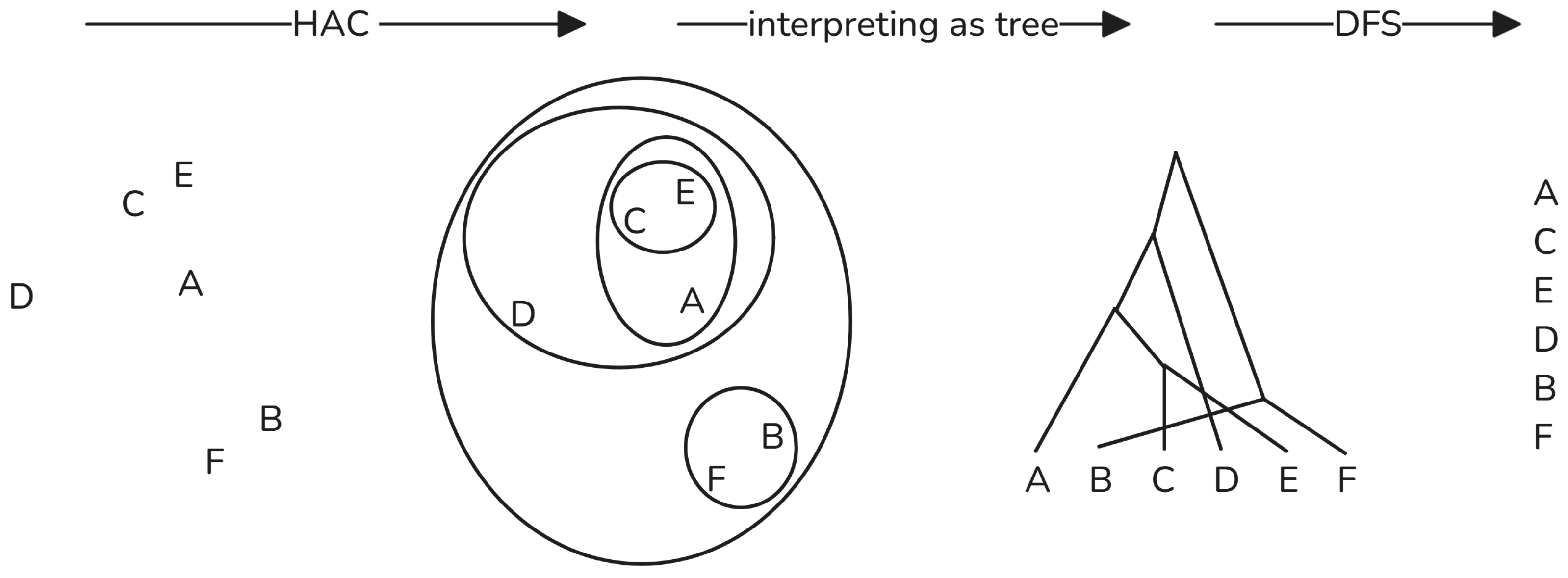
The first step involves clustering the embeddings in a way that enforces “local proximity first.” As we have no prior knowledge of the expected number of clusters, the clustering method should not need specify that. Considering the above, we opted to use hierarchical agglomerative clustering (HAC) [25]. “Hierarchical” means that this method creates clusters from other clusters, constructing a tree of clusters in the process. “Agglomerative” indicates that a bottom-up approach is used in contrast to a divisive one. The algorithm is simple. Initially, each embedding is put in a single element cluster—a leaf node in the tree. From that point, the two most similar clusters are selected and merged. That process continues until there is a single cluster, which can be treated as the root of the tree of clusters. In the context of hierarchical clustering, such similarity is often called linkage. A wide variety of linkages are proposed in the literature. Single linkage involves two clusters that are as similar as the minimum length between their two points. Complete or maximum linkage is based on the maximum distances between all observations of the two sets. Average linkage uses the average distance between points in two clusters. Ward linkage minimizes the variance of the clusters being merged. We tested all of them to discover that despite linkages behaving differently on intentionally created corner-cased benchmarks, all types performed similarly on our datasets.

The second step involves ordering the embeddings from the leaves of the tree. As the most similar clusters were connected first, they are connected lower (closer to the leaves) in the tree. Figure 3 presents an example of this process. The closer to the root the two branches fork, the more different embeddings they contain. That order is preserved by a tree traversal method called depth-first search (DFS) [26].

Algorithm 1 shows full pseudo-code for the proposed method.

Algorithm 1 Semi-online triplet mining.
Require: current cluster $current$, children map $children$  Function DFS(current, children):  if  $children\left[current\right]=null$  then      return $list\left(current\right)$  else      return $concat\left(DFS\right(c,children)$ for c in $children\left[current\right])$  end if
Require: dataset D, buffer-size $bufs$, batch-size $bs$, embedding model E, recalculate-rate r
while $notstop\_condition\left(\right)$  do      $currD\leftarrow D$      while $currDnotempty$ do          $buf\leftarrow pop\_front(currD,bufs)$         $embeddings\leftarrow E\left(x_1^1\right),E\left(x_2^1\right),E\left(x_3^1\right),...$ for $x_i$ in $buf$          $clusters\leftarrow \{\left\{e_1\right\},\left\{e_2\right\},\left\{e_3\right\},...\}$ for $e_i$ from $embeddings$          $children\leftarrow \{\left\{e_1\right\}\to null,\left\{e_2\right\}\to null,\left\{e_3\right\}\to null,...\}$          while $\left|clusters\right|>1$ do             Find the clusters ($c_i$, $c_j$) with the smallest linkage distance             $newCluster\leftarrow c_i\cup c_j$             Delete $c_i$ and $c_j$ from $clusters$             Insert $newCluster$ into $clusters$             $children\left[newCluster\right]\leftarrow \{c_i,c_j\}$          end while          $reordered\_embs\leftarrow DFS(newCluster,children)$          Reorder $buf$ with ordering of $reordered\_embs$          $i\leftarrow 0$          while $i<r$ do             $currBuf\leftarrow buf$             while $currBufnotempty$ do                 $batch\leftarrow pop\_front(currBuf,bs)$                 $triplets\leftarrow mine\_triplets\left(batch\right)$                 $train\_step\left(triplets\right)$             end while             $i\leftarrow i+1$          end while      end while  end while	▹ we use epoch limit and early stopping ▹ populate buffer         ▹ — BEGIN reordering the buffer — ▹ embed first shoes ▹ cluster hierarchy map ▹ we use ’ward’ ▹ newCluster is set to root         ▹ — END reordering the buffer — ▹ we use $semi-hard\cup hard$

4. Datasets and Error Types

This section describes our main, industry-derived dataset and a synthetically generated one, as we conducted experiments on both. It also reviews the compliance of these datasets with triplet learning assumptions.

The first dataset is the constantly growing real-life-photography dataset of shoes that Vive Textile Recycling’s machinery captures in an automated fashion. Every shoe is represented by three photographs taken from different angles, as in Figure 4. This is necessary because shoe components are often reused in various models; many models share identical soles, for example. Although high-resolution RGB images are captured and stored, the model operates on smaller thumbnails of 300x145x3 (HxWxC) FP32 tensors (along with a single integer as an identity identifier). The nature of this dataset implies that we possess only two examples per identity, which reduces our representation of intra-identity variance considerably.

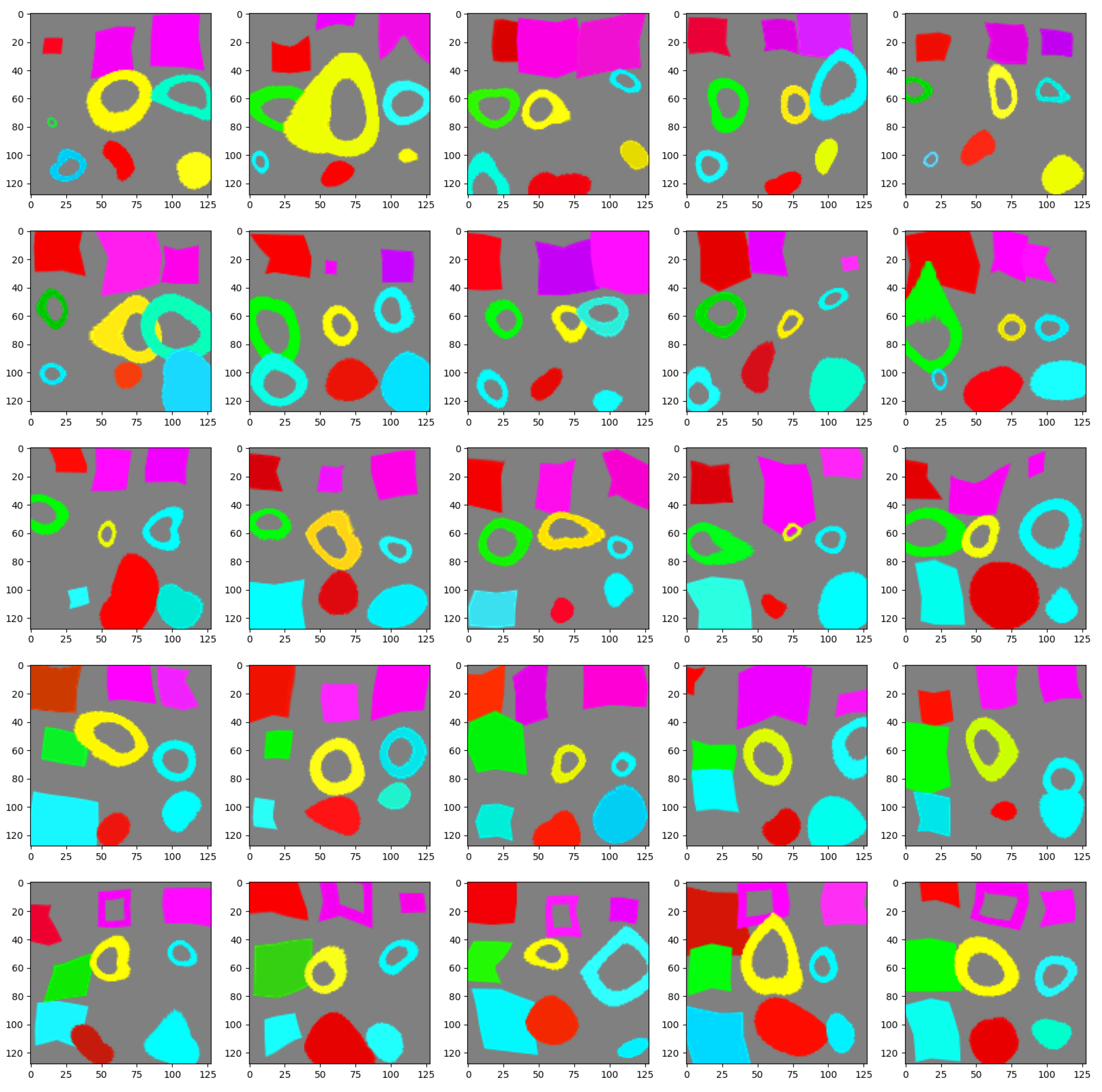
The second dataset is generated synthetically. Every identity is defined by a specific configuration of nine items on the square image. Each item has one of four shapes (filled square, empty square, filled circle, or empty circle) and one of six colors (red, green, blue, cyan, magenta, or yellow). Figure 5 presents examples from this dataset. Examples with the same identity are generated from the canonical form by randomly distorting, translating, resizing, and discoloring all items within the example. The synthetic dataset is not intended to mimic the original dataset, so no measures were taken to align them. The dataset is generated sequentially so that one of the eighteen variables that constitute the current identity (nine shapes and nine colors) is selected and changed randomly to receive a new identity, generating a couple of examples, and then going back to mutating the identity. If an already-existing identity is created, the sampling is repeated. This process produces an already-ordered dataset so that adjacent identities are similar.

In the process of labeling shoes, human labelers are presented with two shoes that come from automatic pre-pairing and must decide whether they are the correct pair. Despite us presenting a single pair-candidate to multiple people, there remains a possibility that they will create false positives. We call this type of error a wrong pair (WP)—a pair in the dataset that is created from shoes that do not create a real pair. A different kind of error can occur when a proper pair of shoes gets labeled as a pair, but an identical pair already exists in the dataset. This creates a distinct identity with shoes that belong to the existing identity. This violates the assumptions of triplet learning because it requires identities to be unique. We call this type of error a hidden pair (HP) because there are hidden (unlabeled) pairs that can be built from shoes belonging to distinct identities. The occurrence of HP errors is a larger problem. That is because with such a large number of shoes being evaluated, there are both unique fashion designs that have a near-zero probability of recurrence in the training set and very popular fashion designs (e.g., sports shoes of mass brands) that occur as several independent pairs in the dataset. Moreover, as the training set gets larger, the probability of making HP errors by adding a new pair to the dataset grows, because the dataset contains an ever-growing reservoir of shoe fashion designs. Simultaneously, it is highly advantageous to keep similar-but-different pairs in the dataset, for the hard triplets to form in greater numbers.

Although we cannot reliably enumerate these errors in our main dataset, we can generate arbitrary levels of them during synthetic dataset generation. We performed a single round of main dataset cleansing in which we selected possible WP and HP cases with a model and sent them to be re-evaluated by a humans.

5. Experiments

We conducted a series of experiments that compared regular online (semi-)hard-triplet mining with the proposed method, which contains the additional step of ordering the dataset periodically. A single experiment involved training an embedding model multiple times and evaluating each instance on ten test sets. The training and test datasets were identical for all runs. Each test dataset comprised 1000 identities with two realizations per identity and 2000 identities with a single realization per identity. For the shoe dataset, that translated into 2000 paired and 2000 unpaired shoes. Shoe pairs in our system are marked either “training pairs” or “test pairs.” We used all training pairs for training but random samples (of the mentioned size) for testing. The main dataset comes in two versions: regular and cleansed. The generated dataset has six versions: some versions have HP and WP errors added, with three error levels for each. The levels of error considered were 0.1%, 1%, and 10%.

Training commences with VGG16 layers being initialized with pretrained weights from ImageNet [27]. Downstream dense layers are initialized with uniform Glorot [28] initialization for kernels and zeros for biases. The loss function is set to the sum of TripletSemiHardLoss and TripletHardLoss. These are TensorFlow (v.2.4.1) [29,30] Addons implementations of the triplet loss function as defined [1]. Both are complex functions responsible for the triplet mining process, not the mere implementation of the triplet loss function. As they are very similar, they share many computationally intensive operations, such as calculating a distance matrix. To prevent the overhead of performing these calculations twice, a new implementation is created to reuse intermediate results, but which still returns the sum of the losses mentioned. The margin parameter of triplet loss is set to 0.2. This loss is minimized using the Adam [31] optimizer. The learning rate for the optimizer starts with 0.001 and is scheduled to decay exponentially ten times per thirty epochs. Training is performed for 300 epochs with early stopping after 30 consecutive epochs with no progress. Our server with one A6000 per VGG16 branch (see [2] for detailed architecture) takes approximately two to three days to complete training.

We perform dataset reordering every five epochs. We use a reordering buffer that fits the whole dataset. That does not mean that we fit the whole dataset into memory at any given point. The current state of the trained embedding model is used to infer the embeddings of the buffer (in our case, the whole training dataset) in batches. Then, our reordering method is applied, and training proceeds normally for another five epochs. 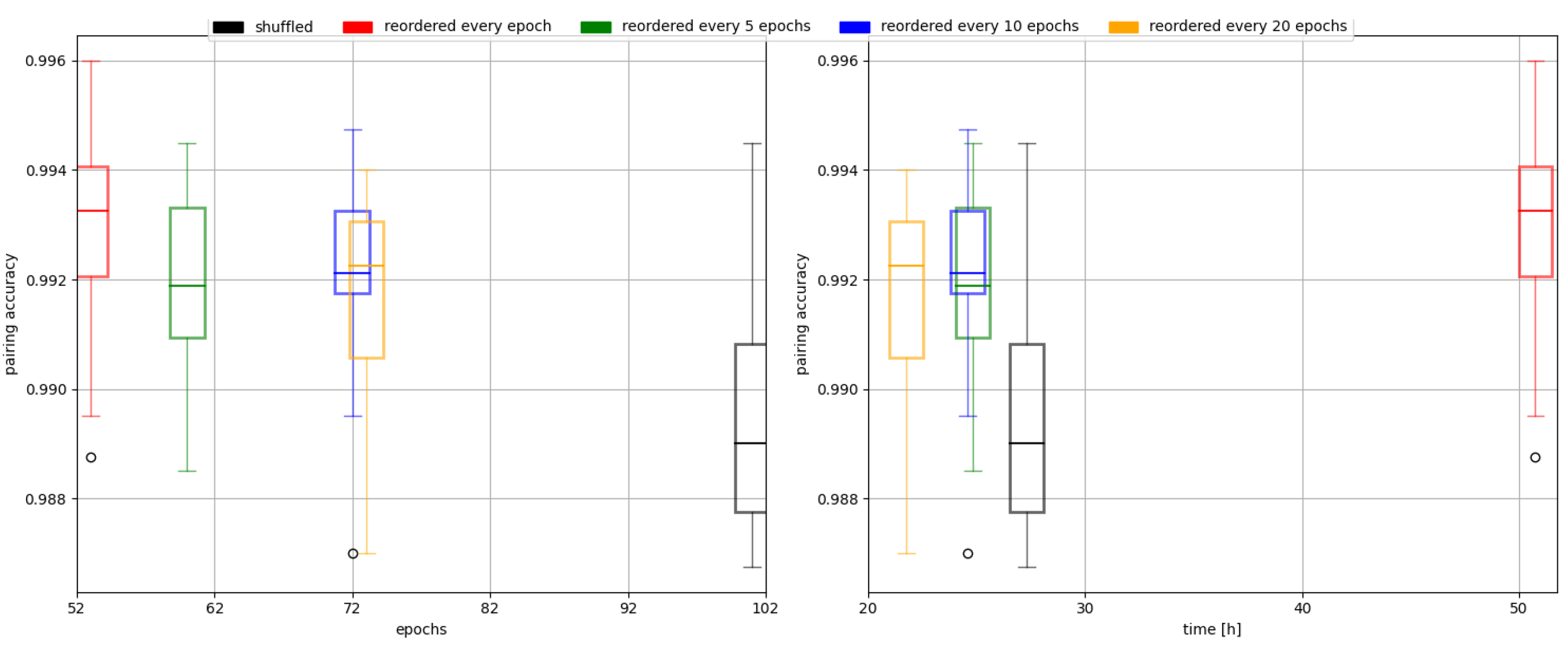Figure 6 shows how reordering frequency affects pairing accuracy and training time.

The validation metric is pairing accuracy, described in [2]. It is a fraction of shoes from a testing set that were paired correctly with another shoe or correctly left unpaired, as the test set can contain single shoes (or unpaired shoes). This metric is test-dataset-size-sensitive, which is unusual. For accuracy or mean squared error, the dataset size is irrelevant because no dependency between examples exists. We may also consider the growing number of all possible pairings in datasets of growing size, from which a pairing method must select one to score 100%.

The test sets for the generated data comprise identities generated consecutively; therefore, they are similar, which makes this a particularly challenging task—even for a human.

We hypothesized in the Section 3 of this article that the efficiency of our method is based on increased ability to identify hard triplets. As we only have two examples per identity, selecting a positive example for any triplet is obvious (there is only one candidate), so identifying a hard negative is the only degree of freedom and the only challenge. The harder the negative, the closer its embedding is to the anchor example’s embedding. To prove that our method enables us to identify harder negatives (and therefore triplets), we excluded the embedding network and its training from the equation by skipping to a dataset that already comprises embeddings randomly sampled from a multi-dimensional unit hypersphere. We then batched that dataset, and for each example in a mini-batch, we found the distance from the closest neighbor, which would translate into a hard negative. We then compared the distributions of these nearest-neighbor distances with and without the use of the proposed ordering step. This experiment was repeated for different dataset and mini-batch sizes.

6. Results

Regarding the main dataset, we observed a change in mean pairing accuracy from 98.95% to 99.17%: a minor but statistically significant (p = 0.0004) improvement. This is a reduction in the pairing error of 20.95%. Cleansing the main dataset in conjunction with our method resulted in a mean pairing accuracy of 99.35% (p= 0.00009) and a further drop in pairing error of 21.68%. The cumulative error reduction is 38.09%, which is relevant in business terms. Figure 7 shows the results of the proposed method applied to the main dataset.

Experiments on the synthetic dataset demonstrate similar trends. As the task was to pair the test dataset with highly similar examples (the generation order was preserved), the task was highly challenging. Regular triplet learning with online (semi-)hard mining is trained on a shuffled training dataset; therefore, on average, only a low number of similar identities end up in each mini-batch, which renders the mining phase ineffective. Despite the initial shuffling of the dataset, our method managed to reorder it so that many more similar identities ended up in the same mini-batch, which enabled the hard-triplet mining step to build harder triplets. The third approach of running triplet learning without shuffling the dataset, therefore feeding it to training in its original order, ideally ordered by similarity, is possible only because the dataset is generated. In the real world, a training dataset does not come ordered. In most cases, our method yields results similar to those of that ideal but artificial control case and better than the random order in every case.

Our experiment on the generated dataset demonstrates the importance of hard triplets clearly. In this setup, both the training and test sets are built from consecutive, therefore similar (difficult to distinguish) identities. During training, the dataset gets shuffled and batched. This process results in random, nonsimilar identities getting batched together. Triplet mining working at the batch level is unable to mine enough hard triplets for training to succeed (this explains the poor result for the “shuffled” case presented in Figure 8). Because the identities in the batch are so easily distinguishable, the network has no incentive to include fine-grained features in the resulting embedding—instead settling for more coarse-grained features, as they are enough on average for training on mini-batches. Examples of the high-level features in this case might be overall (average) color or brightness instead of more complex features that consider colors and shapes simultaneously. This can be overcome by the use of a larger mini-batch (with bigger samples, there is a greater probability of selecting similar identities) or using the proposed method. The advantage of our method is that it requires no additional GPU memory.

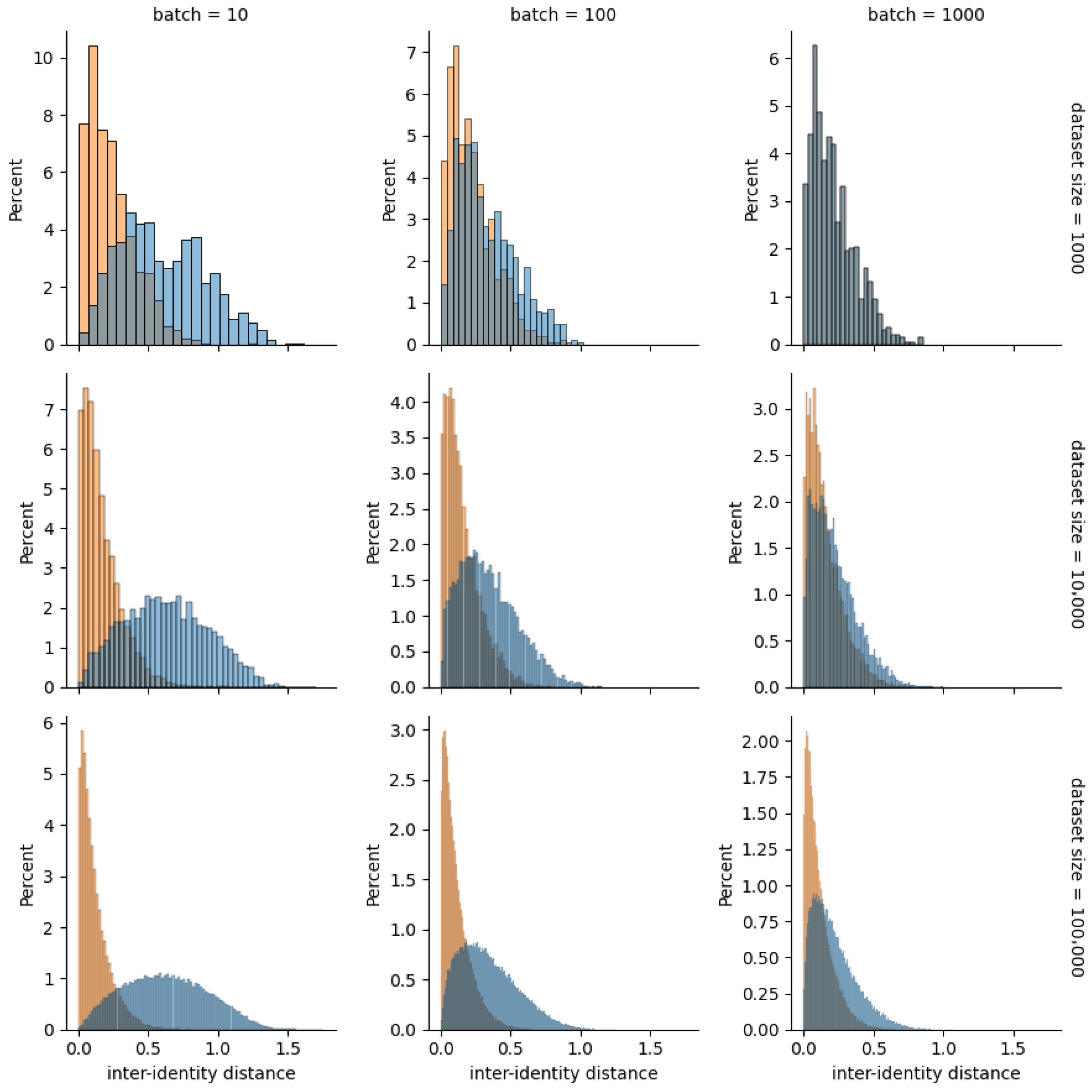
The results of our second experiment concerning the distribution of distances from the closest example (with a different identity) within a mini-batch align with our predictions. Our method yields distributions shifted toward lower distances, thus including many more hard negatives for online (semi-)hard-triplet mining to find. Figure 9 suggests that the difference is more pronounced for smaller mini-batches (left column) and larger datasets (bottom row). In a small-mini-batch scenario without reordering, there is little probability of similar-but-different identities meeting. A larger dataset simply means a higher chance of hard-negative existing (globally)—and when it does, the proposed method capitalizes on that fact by increasing the probability of it falling into a proper mini-batch. When a mini-batch is as large as a whole dataset, our method becomes equivalent to vanilla online triplet mining (top right).

7. Summary

Our previous article presented the design of a solution that is suitable for real-time shoe stream pairing using a deep neural network to transform them into embeddings and cluster them. This article explores the subject more deeply by searching for creative ways of lowering pairing error. We propose a semi-online method for enhancing triplet learning by tweaking the algorithm for building challenging triplets. Our method stems from online (semi-)hard-triplet mining but adds the extra step of (offline) reordering the examples immediately before batching. Reordering uses hierarchical agglomerative clustering and depth-first search traversal to ensure that the maximum number of (semi-)hard triplets can be mined by clumping similar identities together. Our method combines online mining’s ability to use the most recent embeddings calculated by the current state of the model with offline mining’s broader (than a single mini-batch) search for similar-but-different identities. We proved that this semi-online approach yields better results than regular online triplet mining for our particular dataset, as well as generalizing well to artificially generated benchmarking datasets. We see no reason why this method would not generalize well to any application.

References

- Schroff, F.; Kalenichenko, D.; Philbin, J. FaceNet: A Unified Embedding for Face Recognition and Clustering. In Proceedings of the IEEE Conference on Computer Vision and Pattern Recognition, Boston, MA, USA, 7–12 June 2015; pp. 815–823. [Google Scholar]
- Kozłowski, M.; Buczkowski, P.; Brzeziński, P. Novel Process of Shoe Pairing Using Computer Vision and Deep Learning Methods. In Digital Interaction and Machine Intelligence; Lecture Notes in Networks and Systems; Springer: Cham, Switzerland, 2022; Volume 710. [Google Scholar]
- Faghih, E.; Saki, Z.; Moore, M. A Systematic Literature Review—AI-Enabled Textile Waste Sorting. Sustainability 2025, 17, 4264. [Google Scholar] [CrossRef]
- Liu, Z.; Li, W.; Wei, Z. Qualitative classification of waste textiles based on near infrared spectroscopy and the convolutional network. Text. Res. J. 2020, 90, 1057–1066. [Google Scholar] [CrossRef]
- Cura, K.; Rintala, N.; Kamppuri, T.; Saarimäki, E.; Heikkilä, P. Textile recognition and sorting for recycling at an automated line using near infrared spectroscopy. Recycling 2021, 6, 11. [Google Scholar] [CrossRef]
- Li, W.; Wei, Z.; Liu, Z.; Du, Y.; Zheng, J.; Wang, H.; Zhang, S. Qualitative identification of waste textiles based on near-infrared spectroscopy and the back propagation artificial neural network. Text. Res. J. 2021, 91, 2459–2467. [Google Scholar] [CrossRef]
- Noh, S.K. Recycled clothing classification system using intelligent IoT and deep learning with AlexNet. Comput. Intell. Neurosci. 2021, 2021, 5544784. [Google Scholar] [CrossRef] [PubMed]
- Furferi, R.; Servi, M. A machine vision-based algorithm for color classification of recycled wool fabrics. Appl. Sci. 2023, 13, 2464. [Google Scholar] [CrossRef]
- Bhoomika; Verma, G. Optimizing EfficientNetB0 for Shoe Brand Identification: A Comparative Analysis. In Proceedings of the 2024 Second International Conference Computational and Characterization Techniques in Engineering & Sciences (IC3TES), Lucknow, India, 15–16 November 2024; pp. 1–4. [Google Scholar]
- Gill, K.S.; Sharma, A.; Anand, V.; Gupta, R. Smart Shoe Classification Using Artificial Intelligence on EfficientnetB3 Model. In Proceedings of the 2023 International Conference on Advancement in Computation & Computer Technologies (InCACCT), Gharuan, India, 5–6 May 2023; pp. 254–258. [Google Scholar]
- LeCun, Y.; Boser, B.E.; Denker, J.S.; Henderson, D.; Howard, R.E.; Hubbard, W.E.; Jackel, L.D. Backpropagation Applied to Handwritten Zip Code Recognition. Neural Comput. 1989, 1, 541–551. [Google Scholar] [CrossRef]
- LeCun, Y.; Bengio, Y. Convolutional networks for images, speech, and time series. Handb. Brain Theory Neural Netw. 1998, 3361, 1995. [Google Scholar]
- Radford, A.; Kim, J.W.; Hallacy, C.; Ramesh, A.; Goh, G.; Agarwal, S.; Sastry, G.; Askell, A.; Mishkin, P.; Clark, J.; et al. Learning Transferable Visual Models From Natural Language Supervision. In Proceedings of the 38th International Conference on Machine Learning, Virtual Event, 18–24 July 2021; Volume 139, pp. 8748–8763. [Google Scholar]
- Huang, G.; Liu, Z.; Van der Maaten, L.; Weinberger, K.Q. Densely Connected Convolutional Networks. In Proceedings of the IEEE Conference on Computer Vision and Pattern Recognition, Honolulu, HI, USA, 21–26 July 2017; pp. 4700–4708. [Google Scholar]
- Tan, M.; Le, Q.V. EfficientNet: Rethinking Model Scaling for Convolutional Neural Networks. In Proceedings of the 36th International Conference on Machine Learning, Long Beach, CA, USA, 9–15 June 2019; Volume 97, pp. 6105–6114. [Google Scholar]
- Szegedy, C.; Liu, W.; Jia, Y.; Sermanet, P.; Reed, S.; Anguelov, D.; Erhan, D.; Vanhoucke, V.; Rabinovich, A. Going Deeper with Convolutions. In Proceedings of the IEEE Conference on Computer Vision and Pattern Recognition, Boston, MA, USA, 7–12 June 2015; pp. 1–9. [Google Scholar]
- He, K.; Zhang, X.; Ren, S.; Sun, J. Deep Residual Learning for Image Recognition. In Proceedings of the IEEE Conference on Computer Vision and Pattern Recognition, Las Vegas, NV, USA, 27–30 June 2016; pp. 770–778. [Google Scholar]
- Simonyan, K.; Zisserman, A. Very Deep Convolutional Networks for Large-Scale Image Recognition. In Proceedings of the International Conference on Learning Representations, San Diego, CA, USA, 7–9 May 2015. [Google Scholar]
- Lin, M.; Chen, Q.; Yan, S. Network In Network. In Proceedings of the International Conference on Learning Representations, Banff, AB, Canada, 14–16 April 2014. [Google Scholar]
- Bozinovski, S. Reminder of the First Paper on Transfer Learning in Neural Networks, 1976. Informatica 2020, 44, 291–302. [Google Scholar] [CrossRef]
- Hermans, J.R.; Spanakis, G.; Möckel, R. Accumulated Gradient Normalization: A Robust Optimization Technique for Distributed Asynchronous Training. In Proceedings of the First Workshop on Optimization for Machine Learning (OPT 2017), Long Beach, CA, USA, 9 December 2017. [Google Scholar]
- Dantzig, G.B.; Fulkerson, D.R.; Johnson, S.M. Solution of a Large-Scale Traveling-Salesman Problem. Oper. Res. 1954, 2, 393–410. [Google Scholar] [CrossRef]
- van der Maaten, L.; Hinton, G. Visualizing Data using t-SNE. J. Mach. Learn. Res. 2008, 9, 2579–2605. [Google Scholar]
- McInnes, L.; Healy, J.; Melville, J. UMAP: Uniform Manifold Approximation and Projection for Dimension Reduction. arXiv 2018, arXiv:1802.03426. [Google Scholar]
- Johnson, S.C. Hierarchical Clustering Schemes. In Psychometrika; Springer: Chicago, IL, USA, 1967. [Google Scholar]
- Tarjan, R.E. Depth-First Search and Linear Graph Algorithms. SIAM J. Comput. 1972, 1, 146–160. [Google Scholar] [CrossRef]
- Deng, J.; Dong, W.; Socher, R.; Li, L.-J.; Li, K.; Fei-Fei, L. ImageNet: A Large-Scale Hierarchical Image Database. In Proceedings of the IEEE Conference on Computer Vision and Pattern Recognition, Miami, FL, USA, 20–25 June 2009; pp. 248–255. [Google Scholar]
- Glorot, X.; Bengio, Y. Understanding the Difficulty of Training Deep Feedforward Neural Networks. In Proceedings of the International Conference on Artificial Intelligence and Statistics 2010, Sardinia, Italy, 13–15 May 2010. [Google Scholar]
- Abadi, M.; Agarwal, A.; Barham, P.; Brevdo, E.; Chen, Z.; Citro, C.; Corrado, G.S.; Davis, A.; Dean, J.; Devin, M.; et al. TensorFlow: Large-Scale Machine Learning on Heterogeneous Distributed Systems. arXiv 2016, arXiv:1603.04467. [Google Scholar]
- Abadi, M.; Barham, P.; Chen, J.; Chen, Z.; Davis, A.; Dean, J.; Devin, M.; Ghemawat, S.; Irving, G.; Isard, M.; et al. TensorFlow: A system for large-scale machine learning. arXiv 2016, arXiv:1605.08695. [Google Scholar]
- Kingma, D.P.; Ba, J. Adam: A Method for Stochastic Optimization. arXiv 2014, arXiv:1412.6980. [Google Scholar]
Figure 1.
An overview of online triplet mining (top), offline triplet mining (middle), and our method (bottom). Despite integrating the best online and offline mining properties, our method looks much more like online mining than a mix of online and offline.
Figure 2.
A visual representation of regular triplet learning (left) and triplet learning with our semi-online reordering method (right). A single training example (one shoe) is represented as a letter concatenated with a digit. Examples that contain the same letters have the same identity. Color corresponds to the region in the embedding space. The more similar the colors are, the less Euclidean distance between the embeddings there is. Therefore, triplets with a negative example (the third element of the triplet) with a similar color to the anchor (the first element) are harder triplets, which is desirable. Ordering the dataset into a “rainbow” yields batches on which triplet mining can find more hard triplets, visible as more uniformly colored triplets. This is a conceptual, nonquantitative image only.
Figure 3.
The two-step ordering process. Letters represent examples (or more precisely, embedding representation of examples) in the dataset. A small distance between letters represents a high similarity of examples. “Interpreting as tree” is included only for presentation purposes and does not include any data transformation.
Figure 4.
Images of a single shoe from three camera angles.
Figure 5.
Five different realizations (in every row) of five different identities (different rows). Identities in consecutive rows are similar, with only one variable changed—in the second row, for example, the bottom-right circle changes color relative to the first row.
Figure 6.
Performance of different reordering schedules as well as vanilla online (semi-)hard-triplet mining (shuffled). The more frequent the reordering is, the fewer epochs it takes to converge. Despite a lower epoch count, the training time tends to be longer due to growing reordering overhead.
Figure 7.
The pairing accuracies of the methods tested with density estimation plotted. Dots with the same color come from evaluating the same model on different test sets. (*** — p < 0.001 and ****— p < 0.0001).
Figure 8.
The pairing accuracy of different methods on synthetic datasets with different error levels. “Shuffled” (in blue) pertains to the performance of regular triplet learning, which includes shuffling the training dataset. “Ordered” (in orange) pertains to the result of triplet learning on the originally ordered dataset without shuffling. “Reordered” (green) pertains to the performance of our method applied to the shuffled training dataset.
Figure 9.
Distributions of the distances from the closest negative example for each example within a mini-batch. The blue histograms are used to represent the randomly ordered datasets, and the orange histograms are used for datasets reordered using the proposed method.