A Novel Neural Network Framework for Automatic Modulation Classification via Hankelization-Based Signal Transformation

Abstract

Automatic modulation classification (AMC) is a fundamental technique in wireless communication systems, as it enables the identification of modulation schemes at the receiver without prior knowledge, thereby promoting efficient spectrum utilization. Recent advancements in deep learning (DL) have significantly enhanced classification performance by enabling neural networks (NNs) to learn complex decision boundaries directly from raw signal data. However, many existing NN-based AMC methods employ deep or specialized network architectures, which, while effective, tend to involve substantial structural complexity. To address this issue, we present a simple NN architecture that utilizes features derived from Hankelized matrices to extract informative signal representations. In the proposed approach, received signals are first transformed into Hankelized matrices, from which informative features are extracted using singular value decomposition (SVD). These features are then fed into a compact, fully connected (FC) NN for modulation classification across a wide range of signal-to-noise ratio (SNR) levels. Despite its architectural simplicity, the proposed method achieves competitive performance, offering a practical and scalable solution for AMC tasks at the receiver in diverse wireless environments.

1. Introduction

Automatic modulation classification (AMC) is a critical technique in wireless communication systems, serving as a key enabler for dynamic spectrum access and spectrum monitoring [1]. By automatically identifying the modulation schemes of received signals, AMC enables adaptive communication strategies, interference mitigation, and dynamic spectrum management [2,3]. Its importance is further magnified in modern wireless networks, where diverse standards and services coexist, necessitating robust classification under complex channel conditions [1,4]. Emerging technologies such as cognitive radio and dynamic spectrum sharing increasingly rely on AMC for efficient and intelligent spectrum utilization. In particular, adaptive modulation strategies require the receiver to identify modulation formats without prior transmitter coordination, highlighting the need for blind and reliable classification methods capable of operating under uncertainty [5,6]. Such requirements demand classification systems that not only generalize well across modulation types and channel conditions but also operate with low computational cost, especially for real-time or resource-constrained scenarios. As communication environments grow more dynamic and heterogeneous, the development of computationally efficient and reliable AMC algorithms remains a pressing research focus.

Conventional AMC methods can generally be categorized into likelihood-based and feature-based approaches [3,7]. The likelihood-based methods utilize probabilistic models and hypothesis testing to classify modulation schemes accurately under precise channel conditions but often incur prohibitively high computational complexity due to extensive parameter estimation processes, limiting practical deployment [8,9,10]. Conversely, feature-based methods involve classical machine learning (ML) algorithms such as support vector machines (SVMs), decision trees, and the k-nearest neighbors (k-NN) algorithm, which classify handcrafted signal features [3,11]. Although feature-based methods are generally simpler and computationally efficient, they often suffer from limitations related to the discriminative power of manually designed features and restricted learning capabilities inherent in conventional classifiers [12,13]. Moreover, such handcrafted approaches may not generalize well across different channel environments or unforeseen modulation formats.

Recently, neural networks (NNs) have gained considerable attention in AMC research due to their ability to automatically learn hierarchical features directly from raw input signals. By leveraging architectures such as convolutional neural networks (CNNs) [4,14,15], recurrent neural networks (RNNs) [16], and Transformers [17,18], deep learning (DL)-based approaches have demonstrated strong performance across a wide range of channel conditions and signal-to-noise ratio (SNR) levels [4,19]. These models offer greater flexibility and accuracy compared to conventional methods by capturing complex signal patterns without the need for manual feature engineering. In particular, their ability to learn from diverse signal variations makes them suitable for handling the increasing diversity of modulation schemes and channel impairments in wireless systems. Despite these advantages, DL-based AMC models typically require large amounts of data and computational resources and often utilize high-dimensional input representations that limit their practical applicability in real-time or resource-constrained environments. Moreover, many DL frameworks do not explicitly exploit the structured properties of communication signals, potentially overlooking meaningful low-dimensional features.

To overcome these limitations, we propose a novel AMC framework that transforms the received signal into a Hankelized matrix and extracts its singular values to construct a compact and information-rich feature representation. The singular values, obtained through singular value decomposition (SVD), capture key structural properties of the signal and act as a highly discriminative, low-dimensional descriptor. These singular value vectors are then used as direct inputs to a compact NN, trained to classify modulation schemes under wireless channel conditions. A distinctive advantage of the proposed method lies in its ability to effectively leverage the informative nature of singular values, which encapsulate modulation-relevant features while significantly reducing input dimensionality. This compactness allows the use of a simple NN architecture without sacrificing classification performance. In contrast to existing methods that depend on deep or complex models to learn from raw or high-dimensional data, our approach achieves competitive accuracy using a minimal NN structure thanks to the expressiveness of the singular value features. While the proposed NN is not an extremely shallow network, it maintains a relatively compact structure compared to many state-of-the-art AMC architectures, i.e., models based on deep convolutional layers, recurrent units, or Transformer blocks.

The remainder of this paper is organized as follows: Section 2 describes the proposed method, including the system model, problem formulation, and NN design via Hankelization-based preprocessing. Section 3 reports the simulation results, including the experimental setup, comparative analysis of the latent representations produced by different methods, and modulation recognition performance. Finally, Section 4 concludes the paper with a summary of key findings and discussions.

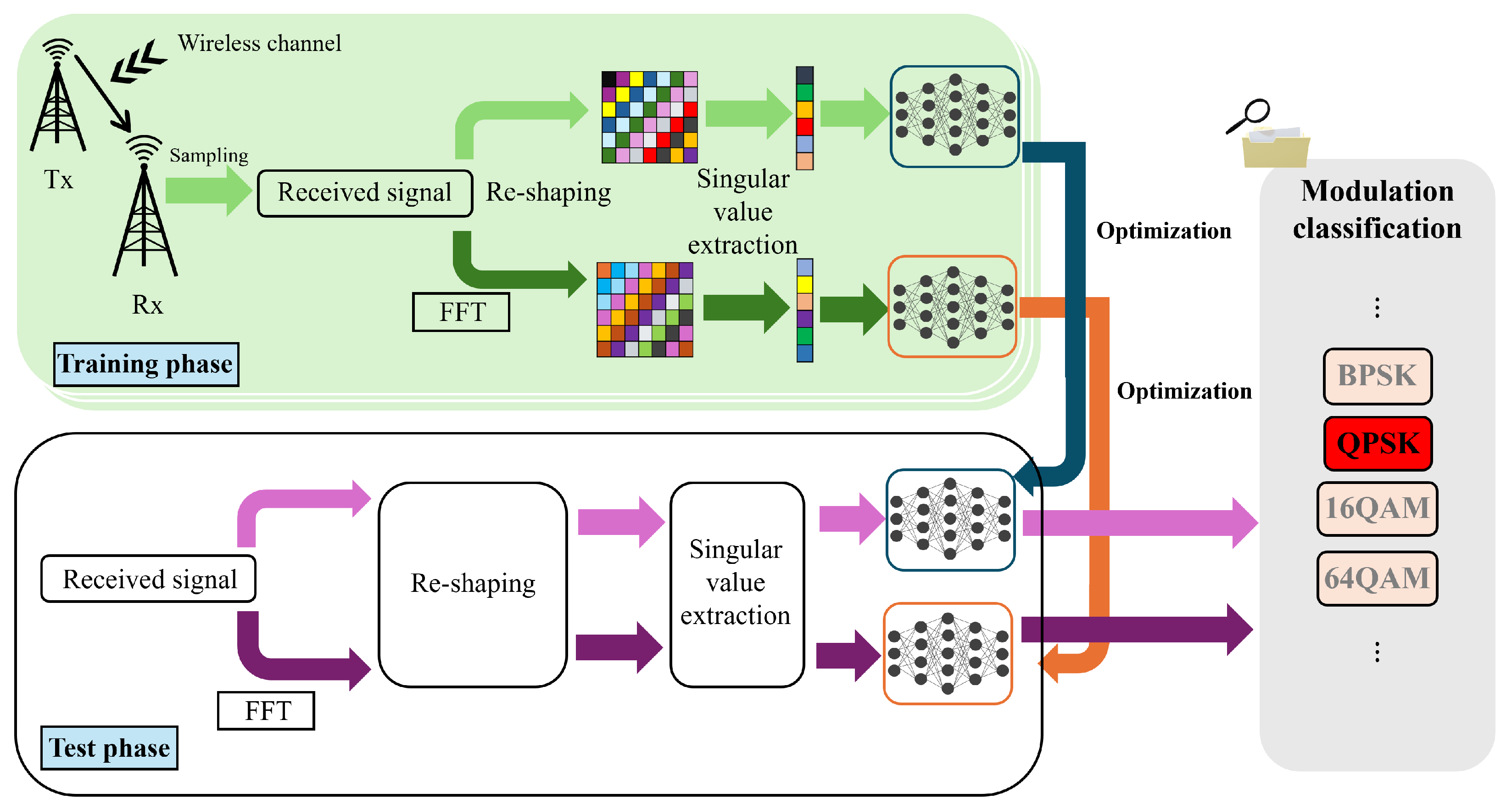
2. Proposed Framework

2.1. System Model and Problem Formulation

Consider the received signal $\mathbf{r}\in {\mathbb{C}}^P$ for a single-input single-output (SISO) system, represented as

$$\mathbf{r}\left[n\right]=e^{j(2\pi f_{err}n{T}_s+{\theta }_{err})}\sum _{l=0}^{L-1}\mathbf{h}\left[l\right]\mathbf{s}[n-l-{\zeta }_{\mathrm{err}}]+\mathbf{w}\left[n\right],\forall n\in \{0,1,\dots ,P-1\},$$

(1)

where L denotes the number of multipaths, $\mathbf{s}$ is the transmitted modulation symbol sequence, $f_{err}$ is the frequency offset, ${\theta }_{err}$ represents the initial phase error, $T_s$ is the sampling rate, $\mathbf{h}$ is the channel impulse response (CIR), ${\zeta }_{err}$ is the timing offset, and $\mathbf{w}$ is additive white Gaussian noise (AWGN) [20].

The objective is to reliably classify the modulation types of received signals embedded in noisy environments. To address this, we first define a Hankelization operator $\hslash :{\mathbb{C}}^{P\times 1}\mapsto {\mathbb{C}}^{P_T\times P_T^{\prime }}$, which transforms a vector $\mathbf{x}$ into a Hankelized matrix $\mathbf{X}$ as follows:

$$\mathbf{X}=\hslash \left(\mathbf{x}\right)\mathrm{s}.\mathrm{t}.\mathbf{X}[i,j]=\mathbf{x}[i+j-1],\forall i,j\in \{1,2,\cdots \},$$

(2)

where $P_T=⌊(P+1/2)⌋$ and $P_T^{\prime }=P-P_T+1$ denote the row and column dimensions of $\mathbf{X}$, respectively, with $⌊·⌋$ indicating the floor operation. We adopt a Hankelized matrix structure that closely approximates a square matrix.

In our proposed framework, we consider two choices for the input vector $\mathbf{x}$ to the Hankelization operator ℏ. First, we apply ℏ directly to the received time-domain signal $\mathbf{r}$ to obtain ${\mathbf{R}}_t=\hslash \left(\mathbf{r}\right)$. Second, we apply the fast Fourier transform (FFT) operator $\mathcal{F}$ to $\mathbf{r}$, resulting in $\tilde{\mathbf{r}}=\mathcal{F}\left(\mathbf{r}\right)$, and construct ${\mathbf{R}}_f=\hslash \left(\tilde{\mathbf{r}}\right)$. This frequency-domain representation is expected to highlight modulation-dependent spectral characteristics, thereby enhancing the separability of different modulation types, especially under noisy conditions. For notational convenience, we denote the resulting Hankelized matrix as ${\mathbf{R}}_d$, where $d\in \{t,f\}$ represents the time-domain t and frequency-domain f variants, respectively. We then apply SVD to ${\mathbf{R}}_d$ as

$${\mathbf{R}}_d={\mathbf{U}}_d{\Sigma }_d{{\mathbf{V}}_d}^H,$$

(3)

where ${\mathbf{U}}_d\in {\mathbb{C}}^{P_T\times P_T}$ and ${\mathbf{V}}_d\in {\mathbb{C}}^{P_T^{\prime }\times P_T^{\prime }}$ are the matrices consisting of $P_T$ left and $P_T^{\prime }$ right singular vectors of ${\mathbf{R}}_d$, respectively. Also, ${\Sigma }_d\in {\mathbb{R}}^{P_T\times P_T^{\prime }}$ is a diagonal matrix whose diagonal elements are the descending ordered singular values, i.e., ${{\sigma }^{\left(\mathit{i}\right)}}_d$, $\forall i\in \{1,\dots ,P_T\}$.

We assume that the extracted singular values ${{\sigma }^{\left(\mathit{i}\right)}}_d$ can effectively form a discriminative latent space suitable for the modulation classification task. To empirically support this assumption, we generate noise-free samples of various modulation types in the MATLAB R2024b environment and visualize their feature distributions using t-distributed stochastic neighbor embedding (t-SNE), a nonlinear dimensionality reduction technique that transforms high-dimensional data into a low-dimensional representation [21].

As shown in Figure 1a, the absolute values of the signal show relatively dispersed and overlapping patterns across different modulation types. In contrast, the singular values derived from the Hankelized matrix in Figure 1b,c exhibit more compact distributions with improved separation between modulation categories, particularly in Figure 1c. These results suggest that the singular values better capture the intrinsic structure of the signal representations.

To provide a quantitative counterpart to the qualitative t-SNE visualization results shown in Figure 1, we compute the silhouette score [22], which evaluates how well each sample is clustered with respect to its assigned label, i.e., modulation type.

$$s\left(i\right)={\displaystyle \frac{b\left(i\right)-a\left(i\right)}{\max \left\{a\right(i),b(i\left)\right\}}},$$

(4)

where $a\left(i\right)$ denotes the average distance from sample i to all other samples in the same class and $b\left(i\right)$ denotes the minimum average distance from i to all samples in any other class. The silhouette score $s\left(i\right)\in [-1,1]$, and the overall score is computed as the average over all samples. Values close to 1 indicate well-separated and compact clusters, while values near or below 0 suggest overlapping or poorly separated classes. As shown in Figure 2, we evaluate the silhouette score using three types of features. In Figure 2a, we vary the number of retained singular values while keeping the Hankelized matrix structure to be nearly square, following the definition in (2). On the other hand, in Figure 2b, we fix the number of singular values to use all available values and vary the row size when forming the Hankelized matrix. In both cases, singular values of ${\mathbf{R}}_f$ (with the FFT-processed signal) consistently yield higher silhouette scores than the other approaches. Notably, as the structure of Hankelized matrix becomes more square-like, the FFT-based features show improved class separability. Therefore, in this work, we follow the Hankelization strategy that attempts to construct a nearly square matrix.

Based on this observation, we design a NN architecture that takes the singular values of the Hankelized matrix as input and performs modulation classification. The overall architecture of the proposed model is illustrated in Figure 3.

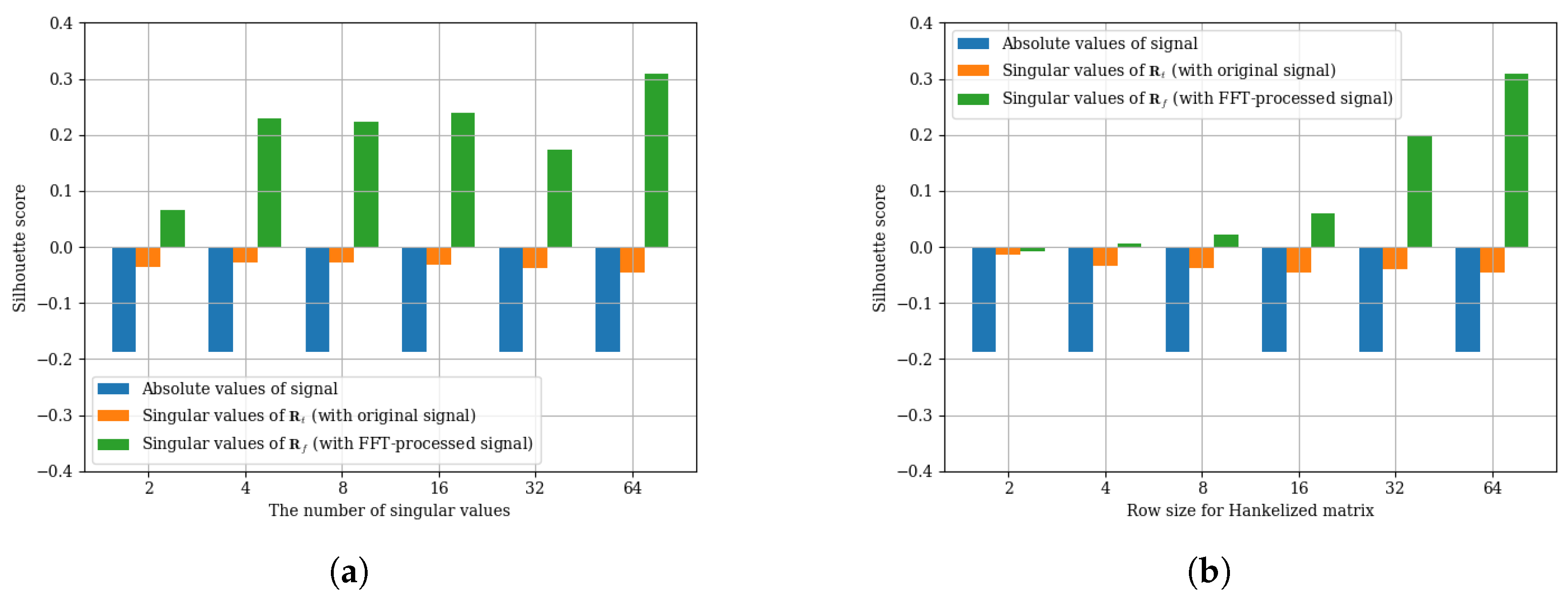
2.2. NN Design via Hankelization-Based Preprocessing

Now, we propose a harmonized framework with Hankelization and NN utilization. The relevant terms are defined as follows:

• $\mathcal{L}$: The loss function.
• $\Theta$: The collection of all trainable parameters, including weight matrices and bias vectors.
• ${\nabla }_{\Theta }$: The parameter gradient computed with respect to $\Theta$.
• C: The number of modulation classes.
• M: The number of training datasets.
• N: The number of test datasets.

Let $c^{\left(m\right)}\in \{1,2,\dots ,C\}$ denote the ground truth modulation class index for the m-th training sample. The corresponding one-hot encoding vector ${\mathbf{e}}^{\left(m\right)}\in {\{0,1\}}^C$ is defined as:

$$\begin{array}{c}\hfill {\mathbf{e}}^{\left(m\right)}\left[c\right]=\left\{\begin{array}{cc}1\hfill & \mathrm{if}c=c^{\left(m\right)},\\ 0\hfill & \mathrm{otherwise}.\end{array}\right.\end{array}$$

(5)

For notational convenience, we define the vector of singular values ${\overline{{\sigma }_d}}^{\left(m\right)}\in {\mathbb{R}}_{+}^{P_T}$ of the Hankelized matrix as follows:

$${\overline{{\sigma }_d}}^{\left(m\right)}=\mathrm{diag}\left({\Sigma }_d\right).$$

(6)

We denote the fully connected (FC) NN model by ${\mathcal{N}}_p$, which is defined using the above terms. Then, the optimized NN model, denoted by ${\mathcal{N}}_p^{\ast }$, is defined as follows:

$${\mathcal{N}}_p^{\ast }=\underset{{\mathcal{N}}_p}{arg\; min}\sum _{m=1}^M\mathcal{L}({\mathbf{e}}^{\left(m\right)},{\mathcal{N}}_p\left({\overline{{\sigma }_d}}^{\left(m\right)}\right)),$$

(7)

where $\mathcal{L}$ is the loss function, and we use the cross-entropy in this work.

To optimize NN model, we adopt the adaptive moment estimation (Adam) optimizer as the update rule for the model; thus, the parameter ${\Theta }_t$ at iteration t is computed as follows:

$${\Theta }_{t+1}\leftarrow {\Theta }_t-\eta ·{\displaystyle \frac{{\mathbf{m}}_{t+1}}{{\sqrt{\mathbf{v}}}_{t+1}+ϵ}},$$

(8)

$$\begin{array}{c}{\mathbf{m}}_{t+1}\leftarrow {\beta }_1{\mathbf{m}}_t+(1-{\beta }_1)\sum _{m\in {\mathcal{B}}_t}{\nabla }_{\Theta }\left(\mathcal{L}({\mathbf{e}}^{\left(m\right)},{\mathcal{N}}_p({\overline{{\sigma }_d}}^{\left(m\right)};{\Theta }_t))\right),\\ \\ {\mathbf{v}}_{t+1}\leftarrow {\beta }_2{\mathbf{v}}_t+(1-{\beta }_2)\sum _{m\in {\mathcal{B}}_t}{\nabla }_{\Theta }{\left(\mathcal{L}({\mathbf{z}}^{\left(m\right)},{\mathcal{N}}_p({\overline{{\sigma }_d}}^{\left(m\right)};{\Theta }_t))\right)}^2,\end{array}$$

(9)

where ${\mathcal{B}}_t$ refers to the set of indices associated with the input/output samples in the current minibatch. The learning rate is denoted by $\eta$, while $\mathbf{m}$ and $\mathbf{v}$ represent the first and second moment estimates, respectively. And ${\beta }_1$ and ${\beta }_2$ are the exponential moving average of momentum and the exponential moving average of root mean square propagation (RMSProp), respectively. Now, in accordance with (7), (8), and (9), we can obtain the optimized ${\mathcal{N}}_p^{\ast }$. Then, the result vector $\widehat{\mathbf{e}}$ from $\overline{{\sigma }_d}$ can be obtained as follows:

$$\widehat{\mathbf{e}}={\mathcal{N}}_p^{\ast }\left(\overline{{\sigma }_d}\right).$$

(10)

Finally, the predicted modulation class index $\widehat{c}$ is determined as the index corresponding to the maximum value of the NN output vector:

$$\widehat{c}=arg\underset{c}{max}\widehat{\mathbf{e}}\left[c\right].$$

(11)

Algorithm 1 shows the procedure of the proposed method. The performance of the optimized NN model ${\mathcal{N}}_p^{\ast }$ is evaluated through numerical simulations in the following section.

Algorithm 1 The Procedure of the Proposed Method

[Training phase]

1:     Collect training dataset ${\left\{({\mathbf{r}}^{\left(m\right)},{\mathbf{e}}^{\left(m\right)})\right\}}_{m=1}^M$.

2:     Select domain $d\in \{t,f\}$ for all samples:                 $d=t$ (time-domain) or $d=f$ (frequency-domain via FFT).

3:     for $m\leftarrow 1$ to M do

4:        Build Hankelized matrix: ${\mathbf{R}}_d^{\left(m\right)}=\left\{\begin{array}{cc}\hslash \left({\mathbf{r}}^{\left(m\right)}\right)\hfill & \mathrm{if}d=t,\hfill \\ \hslash \left(\mathcal{F}\left({\mathbf{r}}^{\left(m\right)}\right)\right)\hfill & \mathrm{if}d=f.\hfill \end{array}\right.$

5:        Compute SVD based on (3): ${\mathbf{R}}_d^{\left(m\right)}={\mathbf{U}}_d{\Sigma }_d{\mathbf{V}}_d$.

6:        Extract the vector consisting of singular values based on (6)            ${\overline{{\sigma }_d}}^{\left(m\right)}=\mathrm{diag}\left({\Sigma }_d\right)$.

7:     end for

8:     Optimize NN ${\mathcal{N}}_p$ based on (7), (8), and (9).

[Test phase]

9:     Collect test dataset ${\left\{{\mathbf{r}}^{\left(n\right)}\right\}}_{n=1}^N$.

10:     Employ the same domain $d\in \{t,f\}$ as chosen during training phase.

11:     for  $n\leftarrow 1$ to N do

12:        Build Hankelized matrix ${\mathbf{R}}_d^{\left(n\right)}$ as in Step 4.

13:        Make the input vector ${\overline{{\sigma }_d}}^{\left(n\right)}$ referring to Step 5 and 6.

14:        Predict modulation class index based on (10) and (11):${\widehat{\mathbf{e}}}^{\left(n\right)}={\mathcal{N}}_p^{\ast }\left({\overline{{\sigma }_d}}^{\left(n\right)}\right)$,                            ${\widehat{c}}^{\left(n\right)}=arg{max}_c{\widehat{\mathbf{e}}}^{\left(n\right)}\left[c\right]$.

15:     end for

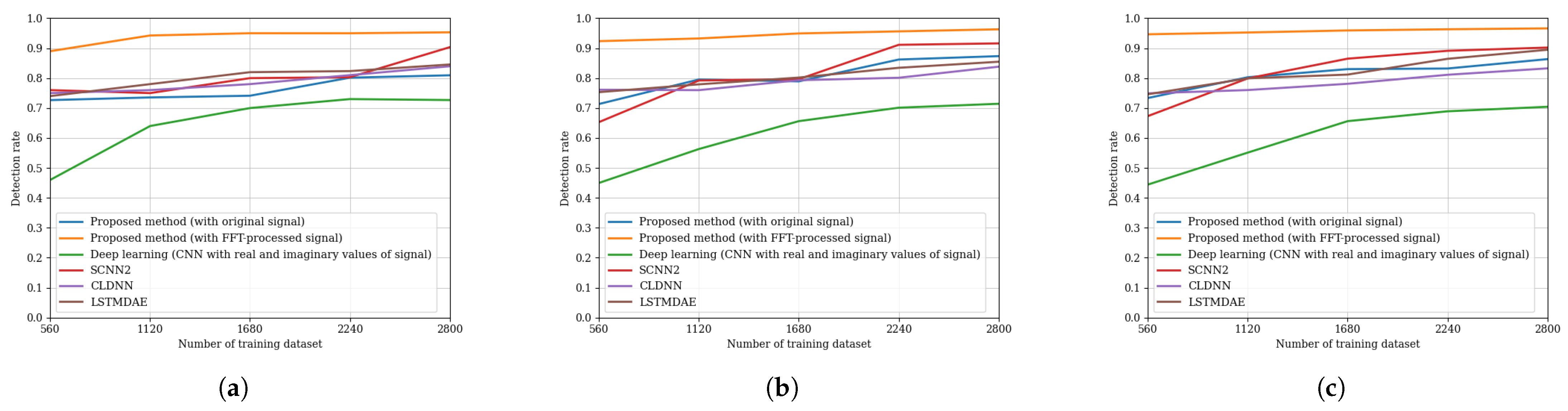
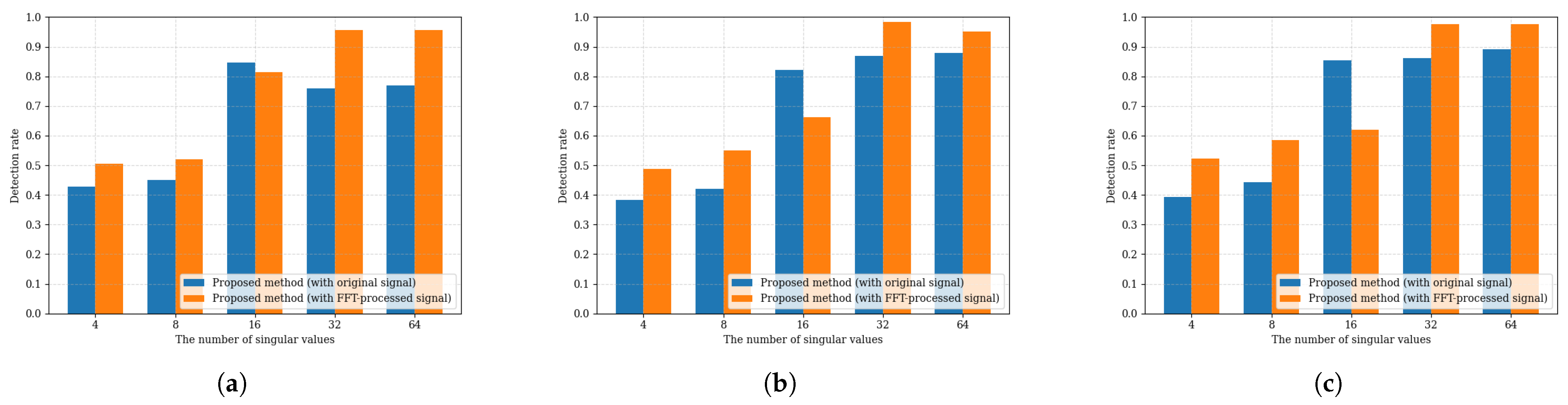
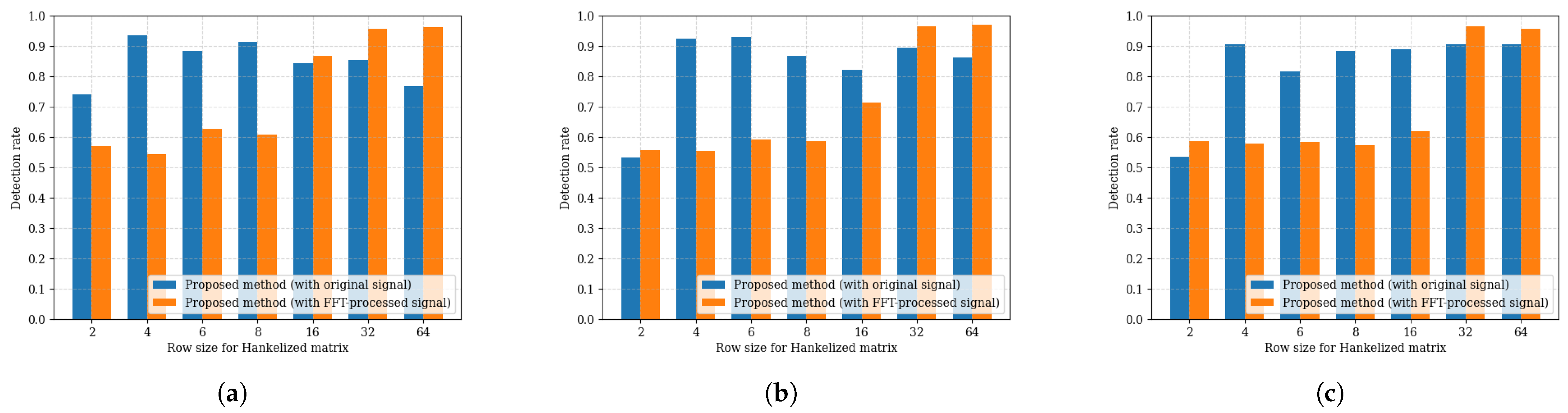
3. Simulation Results

3.1. Simulation Configurations

The experiments in this study are conducted using the widely used RadioML2016.10a dataset introduced in [23], which is commonly adopted for evaluating AMC performance. The dataset configuration, including channel model parameters and signal generation settings, is summarized in

Table 1. Settings of the RadioML2016.10a dataset [20,23].

Parameter	Value
Channel model	Rician fading
K-factor	4 dB
Sampling rate $T_s$	200 kHz
Number of multipaths L	3
Doppler frequency	max = 1 Hz
Initial phase error ${\theta }_{err}$	U(0, $2\pi$)
Frequency offset $f_{err}$	Standard deviation per sample = $0.01$, Maximum deviation: 500 Hz
Timing offset ${\zeta }_{err}$	Standard deviation per sample = $0.01$, Maximum deviation: 500 Hz
Number of samples per modulation per SNR	1000
Length of samples	128
SNR	$-20$ to 20 dB in steps of 2 dB

. Additionally,

Table 2. Default configuration in the experiments.

Parameter	Value
Data split (per modulation class)	70% training/10% validation/20% testing
NN depth d	3
NN width $P_W$	24
Epochs	120
Mini-batch size	64
NN connection type	FC
Learning rate	${10}^{-2}$
Activation function	Hyperbolic tangent function
Loss function	Cross-entropy
Optimizer	Adam
${\beta }_1$, ${\beta }_2$	$0.9$, $0.99$
$ϵ$	${10}^{-8}$
Experimental setup	Python 3.10.16, PyTorch 2.5.1, CUDA 12.1, cuDNN 9.1.0, NVDIA RTX A4000 GPU, Intel Core i9-11900K CPU

presents the default experimental setup, including the NN architecture, hyperparameters, and computational environment.

The performance metric employed in this paper is the detection rate, defined as the ratio of correctly classified samples to the total number of test samples N. The detection rate is computed as

$$\mathrm{detection}\mathrm{rate}={\displaystyle \frac{\mathrm{card}\{n\mid {\widehat{c}}^{\left(n\right)}=c^{\left(n\right)}\}}{N}},\forall n\in \{1,\cdots ,N\},$$

(12)

where $\mathrm{card}\{·\}$ denotes the cardinality of the set. This metric reflects the classification accuracy across all test samples.

The effectiveness of the proposed method was assessed through comparison with four baseline methods:

• Deep learning (CNN with real and imaginary values of the signal: The NN-based method that utilizes a CNN architecture, in which the real and imaginary parts of the input signal are treated as two separate input channels. This structure follows the design presented in [24].
• SCNN2: The NN-based method that transforms raw complex signals into spectrogram images via discrete short-time Fourier transform (STFT), applies Gaussian filtering for noise reduction, and performs classification using a dedicated CNN architecture optimized for time-frequency representations, as described in [14].
• CLDNN: The NN-based method that combines convolutional layers for local feature extraction, long short-term memory (LSTM) layers for modeling temporal dependencies, and FC layers for classification. This hybrid architecture leverages both spatial and temporal information embedded in the received signal, following the design principles in [16].
• LSTMDAE: The NN-based method that employs a denoising autoencoder (DAE) based on LSTM networks, which learns robust latent representations of noisy signals through temporal masking and reconstruction. The decoder output is jointly optimized with a modulation classification objective, thereby improving classification performance under noisy conditions, as introduced in [25].

Among the 11 modulation types in the RadioML2016.10a dataset, we select BPSK, QPSK, 16QAM, and 64QAM for evaluation. These schemes are chosen to cover both phase modulation and amplitude–phase combined modulation, allowing us to assess classification performance using a simple NN and minimal preprocessing.

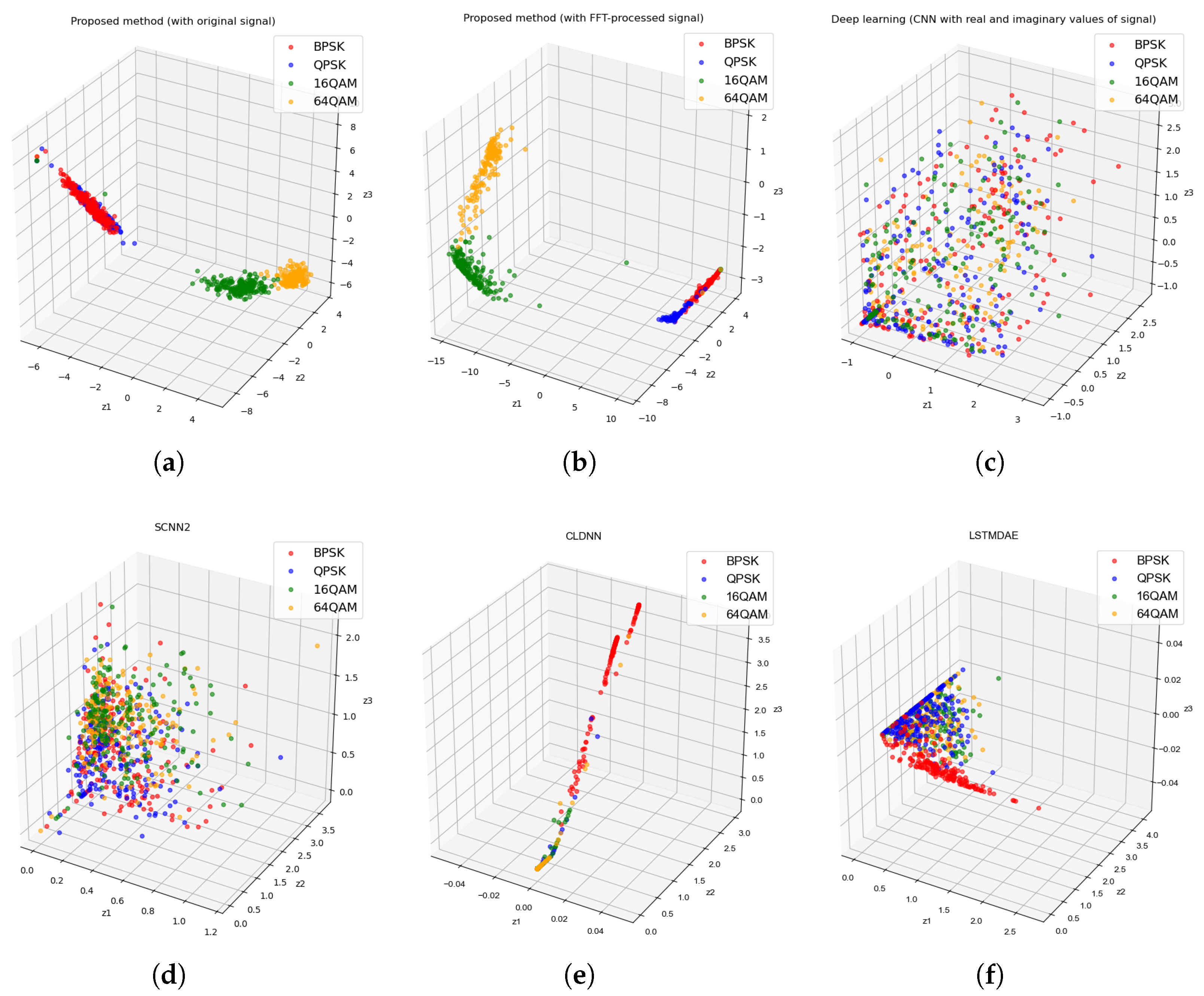
3.2. Empirical Latent Space Comparison Across Models

To investigate the feature representation capability of each model, we empirically visualize the latent vectors $\mathbf{z}\in {\mathbb{R}}^3$ obtained from the final hidden layer prior to classification. Let $\mathcal{G}$ denote the set of considered models, including the proposed methods and three baseline schemes. For each model $g\in \mathcal{G}$, the optimized NN model is denoted by ${\mathcal{N}}_g^{\ast }$, which can be decomposed as

$${\mathcal{N}}_g^{\ast }={\mathcal{C}}_g\circ f_{\mathrm{latent}}^{\left(g\right)}$$

(13)

where ∘ is the composition operator of the function, $f_{\mathrm{latent}}^{\left(g\right)}(·)$ denotes the feature mapping function up to the penultimate layer, and ${\mathcal{C}}_g(·)$ is the final classification layer of model g.

Given a model-specific input $\mathbf{y}$, the corresponding latent feature vector is obtained as

$$\mathbf{z}=f_{\mathrm{latent}}^{\left(g\right)}\left(\mathbf{y}\right).$$

(14)

To facilitate visualization, the output dimension of $f_{\mathrm{latent}}^{\left(g\right)}$ was fixed to 3 for all $g\in \mathcal{G}$ in this analysis. Note, however, that the original models used for classification in the next subsection employ higher-dimensional latent spaces.

Figure 4 shows the resulting 3D scatters of latent vectors $\mathbf{z}\in {\mathbb{R}}^3$, categorized by modulation classes, i.e., BPSK, QPSK, 16QAM, and 64QAM. Each subfigure corresponds to a different model $g\in \mathcal{G}$. As seen in Figure 4a,b, the proposed methods result in more structured and discriminative embeddings for modulation types, whereas the baseline models exhibit more entangled and less separable latent representations.

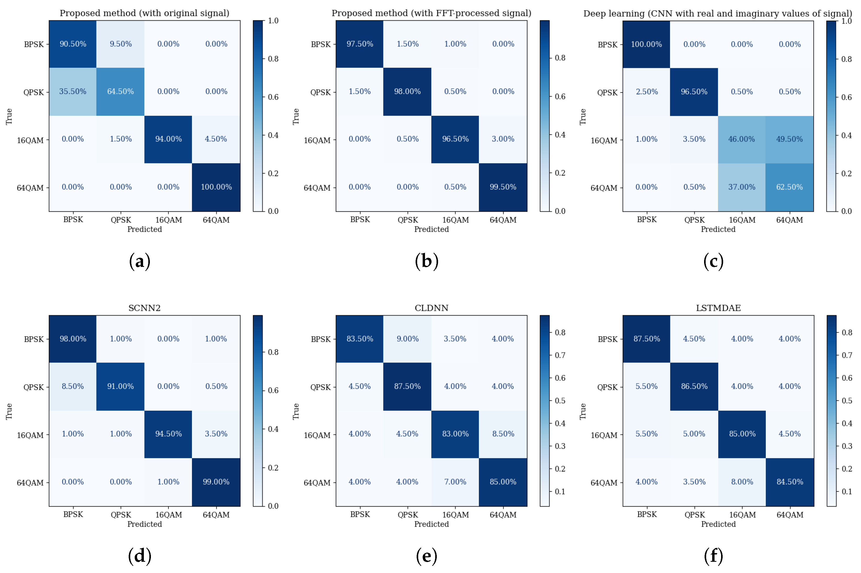
3.3. Performance Evaluation for Modulation Recognition

In Figure 5, confusion matrices are shown for six methods, each evaluated at 10 dB SNR conditions across four modulation schemes. In each matrix, rows indicate the ground-truth modulation classes, whereas columns correspond to the predicted classes. For instance, as seen in Figure 5a a value of $94.0\%$ in the third row and third column indicates that $94.0\%$ of 16QAM samples were correctly classified as 16QAM, whereas $6.0\%$ were incorrectly classified as 16QAM, and so forth. As shown in Figure 5b, the proposed method (with the FFT-processed signal) achieves the highest classification accuracy across almost all modulation types compared to other baseline methods. Among the baseline methods, SCNN2 in Figure 5d shows competitive performance, likely due to its spectrogram-based preprocessing with Gaussian filtering, which effectively suppresses noise. While the proposed method with original signals (Figure 5a) does not employ explicit denoising, it still achieves high accuracy for BPSK, 16QAM, and 64QAM, while exhibiting limited discriminability between QPSK and BPSK.

Figure 6 shows the detection rate according to the number of training datasets. For instance, a total of 2800 training samples corresponds to 700 samples per modulation class when four modulation types are considered.

Across all SNR levels and training sizes, the proposed method (with FFT-processed signal), shown in orange, consistently achieves the highest detection rate. As shown in Figure 6a, even when trained with only 560 samples in total—corresponding to 140 samples per class under the SNR condition of 4 dB—the proposed method (with FFT-processed signal) maintains a detection rate approaching $0.9$, demonstrating strong robustness under limited data availability.

Table 3. Mean of detection rate ± standard deviation according to SNR.

SNR [dB]	Proposed Method (with Original Signal)	Proposed Method (with FFT-Processed Signal)	Deep Learning (CNN with Real and Imaginary Values of Signal)	SCNN2	CLDNN	LSTMDAE
−20	$0.2500\pm 0.0000$	$0.2500\pm 0.0000$	$0.2460\pm 0.0102$	$0.2500\pm 0.0196$	0.2545 ± 0.0113	0.2490 ± 0.0123
−18	$0.2500\pm 0.0000$	$0.2500\pm 0.0000$	$0.2428\pm 0.0149$	$0.2636\pm 0.0167$	0.2529 ± 0.0099	0.2454 ± 0.0066
−16	$0.3046\pm 0.0164$	$0.2504\pm 0.0011$	$0.2826\pm 0.0199$	$0.3299\pm 0.0198$	0.3394 ± 0.0138	0.2476 ± 0.0054
−14	$0.3881\pm 0.0146$	$0.3433\pm 0.0934$	$0.4354\pm 0.0181$	$0.4505\pm 0.0152$	0.4627 ± 0.0282	0.2984 ± 0.0692
−12	$0.5205\pm 0.0217$	$0.5630\pm 0.0279$	$0.5496\pm 0.0215$	$0.5693\pm 0.0103$	0.5888 ± 0.0176	0.6123 ± 0.0145
−10	$0.6560\pm 0.0097$	$0.6671\pm 0.0164$	$0.6389\pm 0.0112$	$0.6491\pm 0.0175$	0.6834 ± 0.0176	0.6912 ± 0.0131
−8	$0.7206\pm 0.0056$	$0.7036\pm 0.0211$	$0.6894\pm 0.0128$	$0.6915\pm 0.0208$	0.7140 ± 0.0077	0.7251 ± 0.0078
−6	$\mathbf{0}.\mathbf{7394}\pm 0.0083$	$\mathbf{0}.\mathbf{7334}\pm 0.0060$	$0.7184\pm 0.0138$	$0.7129\pm 0.0160$	0.7292 ± 0.0146	0.7329 ± 0.0148
−4	$0.7395\pm 0.0052$	$0.7380\pm 0.0038$	$0.7205\pm 0.0142$	$0.7336\pm 0.0092$	0.7274 ± 0.0082	0.7409 ± 0.0138
−2	$0.7346\pm 0.0040$	$0.7285\pm 0.0121$	$0.7125\pm 0.0264$	$0.7674\pm 0.0321$	0.7264 ± 0.0098	0.7428 ± 0.0609
0	$0.7406\pm 0.0137$	$\mathbf{0}.\mathbf{8194}\pm 0.0445$	$0.6911\pm 0.0217$	$0.8005\pm 0.0418$	0.7297 ± 0.0655	0.7316 ± 0.0119
2	$0.8102\pm 0.0317$	$\mathbf{0}.\mathbf{9084}\pm 0.0171$	$0.6986\pm 0.0277$	$0.8603\pm 0.0564$	0.8229 ± 0.0843	0.8408 ± 0.0097
4	$0.8085\pm 0.0379$	$\mathbf{0}.\mathbf{9439}\pm 0.0147$	$0.7368\pm 0.0180$	$0.9133\pm 0.0500$	0.8396 ± 0.0614	0.8456 ± 0.0196
6	$0.8569\pm 0.0346$	$\mathbf{0}.\mathbf{9614}\pm 0.0046$	$0.7458\pm 0.0261$	$0.9151\pm 0.0493$	0.8306 ± 0.0560	0.8508 ± 0.0120
8	$0.8641\pm 0.0217$	$\mathbf{0}.\mathbf{9574}\pm 0.0132$	$0.6789\pm 0.0256$	$0.8835\pm 0.0558$	0.8316 ± 0.0607	0.8545 ± 0.0112
10	$0.8870\pm 0.0395$	$\mathbf{0}.\mathbf{9699}\pm 0.0073$	$0.7286\pm 0.0240$	$0.9261\pm 0.0118$	0.8482 ± 0.0125	0.8448 ± 0.0182
12	$0.8899\pm 0.0165$	$\mathbf{0}.\mathbf{9484}\pm 0.0561$	$0.6784\pm 0.0234$	$0.9089\pm 0.0558$	0.8341 ± 0.0159	0.8512 ± 0.0281
14	$0.8698\pm 0.0214$	$\mathbf{0}.\mathbf{9647}\pm 0.0106$	$0.6959\pm 0.0157$	$0.8958\pm 0.0434$	0.8336 ± 0.0535	0.8619 ± 0.0221
16	$0.8656\pm 0.0282$	$\mathbf{0}.\mathbf{9669}\pm 0.0064$	$0.6790\pm 0.0252$	$0.9014\pm 0.0544$	0.8326 ± 0.0676	0.8945 ± 0.0196
18	$0.8473\pm 0.0536$	$\mathbf{0}.\mathbf{9623}\pm 0.0093$	$0.6876\pm 0.0226$	$0.9111\pm 0.0329$	0.8403 ± 0.0687	0.8898 ± 0.0159

presents the average detection rate and corresponding standard deviation across 10 independent trials, each conducted with different random seeds, for various SNR levels ranging from $-20$ to 18 dB. The boldfaced values indicate the SNR points where the proposed methods achieve the highest mean detection rate among all evaluated methods. From 0 dB and above, the proposed method (with the FFT-processed signal) demonstrates superiority, yielding the highest detection rates across all conditions in this range. These results collectively validate that the proposed framework, particularly when combined with FFT preprocessing, achieves superior classification performance compared to baseline methods, demonstrating robustness and stability across various SNR conditions.

Figure 7 shows the test error curves across training epochs. The proposed method (with FFT-processed signal), shown in orange, consistently exhibits the fastest convergence and lowest test error across all SNR levels. Notably, under the SNR condition of 4 dB, as shown in Figure 7a, the proposed method (with FFT-processed signal) achieves a near-minimal test error within 30 epochs. The results highlight that the FFT-based method achieves faster convergence and learns robust, discriminative features effectively across varying conditions.

Figure 8 shows the detection performance of the proposed method under various SNR levels, with respect to the number of retained singular values. The Hankelized matrix is constructed to be approximately square, while the number of singular values is varied to assess its influence on classification accuracy. Across all SNR conditions, the detection rate improves as more singular values are retained, highlighting the benefit of preserving sufficient spectral information. Furthermore, the FFT-processed variant consistently outperforms the original signal variant, particularly when a sufficient number of singular values is used.

Figure 9 presents the detection performance of the proposed method under varying row sizes of the Hankelized matrix across different SNR conditions. The number of singular values retained is fixed to the row dimension, while the row size is varied to assess the effect of the matrix shape. The results indicate that a well-chosen row size, even without strictly enforcing a near-square matrix structure, can still lead to a high detection rate. Notably, the FFT-processed variant achieves relatively higher accuracy in most SNR settings when the row size is sufficiently large.

These observations suggest that high detection performance can be attained by appropriately selecting the number of singular values and the row size of the Hankelized matrix.

Table 4. Comparison of computational complexity in terms of FLOPs and the number of parameters.

Method	FLOPs	# Params
Proposed method (with original signal)	$5.72\times {10}^3$	$2.86\times {10}^3$
Proposed method (with FFT-processed signal)	$5.72\times {10}^3$	$2.86\times {10}^3$
Deep learning (CNN with real and imaginary values of signal)	$2.04\times {10}^6$	$1.58\times {10}^5$
SCNN2	$1.42\times {10}^8$	$1.73\times {10}^5$
CLDNN	$7.89\times {10}^6$	$3.50\times {10}^4$
LSTMDAE	$3.53\times {10}^6$	$1.48\times {10}^4$

presents the computational complexity of each model in terms of the number of floating-point operations (FLOPs) and network parameters required for a single inference. Recalling the width of each hidden layer, denoted by $P_W$, and the depth of the NN d, the FLOP complexity of an FC model is given by $\mathcal{O}\left(d{P}_T{P}_W\right)$. Although the proposed methods introduce an additional computational cost of $\mathcal{O}\left(P_T^2{P}_T^{\prime }\right)$ due to singular value extraction via Hankelization, this step is performed as part of offline preprocessing. As shown in Table 4, both variants of the proposed method—one using the original signal and the other using the FFT-processed signal—require only $5.72\times {10}^3$ FLOPs and $2.86\times {10}^3$ parameters, demonstrating significantly lower complexity compared to other baseline methods. In particular, CNN-based architectures such as SCNN2 and CLDNN require up to $1.42\times {10}^8$ and $7.89\times {10}^6$ FLOPs, respectively, with network sizes ranging from $1.73\times {10}^5$ to $3.50\times {10}^4$ parameters. The baseline methods follow the same NN configuration described in Section 3.1, ensuring a fair comparison in terms of network depth and width. The findings highlight that, although a mathematically complex preprocessing step is employed, the proposed method maintains high computational efficiency.

4. Conclusions

In this paper, we proposed a NN-based framework for AMC, incorporatingHankelization preprocessing. The proposed approach transforms the received signals into Hankelized matrices, from which singular values are extracted to form low-dimensional yet informative feature vectors. Two variants of the method were investigated—one based on time-domain signals and the other incorporating frequency-domain features via FFT. These features are then fed into an NN composed of a simple FC structure to perform classification across various SNR environments. The key strength of the proposed framework lies in its ability to effectively extract modulation-relevant features without relying on deep or complex NN architectures. Unlike conventional methods that depend on either handcrafted features or high-capacity models, our approach employs a concise design with minimal layers and moderate width, demonstrating that high performance can still be achieved when combined with appropriate signal representations.

Experimental results confirm that the FFT-enhanced variant consistently achieves the highest detection accuracy across a wide range of SNR levels. Notably, it performs reliably even under low-SNR conditions and with limited training data, maintaining stable detection rates. In addition, the model converges rapidly within a small number of training epochs. Latent space analysis further supports the ability of the model to form well-separated representations across modulation types. In summary, the proposed Hankelization-based AMC framework provides a practical and effective solution by integrating signal structure-aware preprocessing with a simple NN architecture. Future work may extend this framework to broader modulation families or more complex channel environments.

References

1. Gui, G.; Liu, M.; Tang, F.; Kato, N.; Adachi, F. 6G: Opening new horizons for integration of comfort, security, and intelligence. IEEE Wirel. Commun. 2020, 27, 126–132. [Google Scholar] [CrossRef]
2. Dobre, O.A.; Abdi, A.; Bar-Ness, Y.; Su, W. Survey of automatic modulation classification techniques: Classical approaches and new trends. IET Commun. 2007, 1, 137–156. [Google Scholar] [CrossRef]
3. Huynh-The, T.; Pham, Q.V.; Nguyen, T.V.; Nguyen, T.T.; Ruby, R.; Zeng, M.; Kim, D.S. Automatic modulation classification: A deep architecture survey. IEEE Access 2021, 9, 142950–142971. [Google Scholar] [CrossRef]
4. O’Shea, T.J.; Roy, T.; Clancy, T.C. Over-the-air deep learning based radio signal classification. IEEE J. Sel. Top. Signal Process. 2018, 12, 168–179. [Google Scholar] [CrossRef]
5. Häring, L.; Chen, Y.; Czylwik, A. Efficient modulation classification for adaptive wireless OFDM systems in TDD mode. In Proceedings of the 2010 IEEE Wireless Communications and Networking Conference, Sydney, Australia, 18–21 April 2010; pp. 1–6. [Google Scholar]
6. Harper, C.A.; Thornton, M.A.; Larson, E.C. Automatic modulation classification with deep neural networks. Electronics 2023, 12, 3962. [Google Scholar] [CrossRef]
7. Fu, X.; Gui, G.; Wang, Y.; Gacanin, H.; Adachi, F. Automatic modulation classification based on decentralized learning and ensemble learning. IEEE Trans. Veh. Technol. 2022, 71, 7942–7946. [Google Scholar] [CrossRef]
8. Su, W.; Xu, J.L.; Zhou, M. Real-time modulation classification based on maximum likelihood. IEEE Commun. Lett. 2008, 12, 801–803. [Google Scholar] [CrossRef]
9. Xu, J.L.; Su, W.; Zhou, M. Likelihood-ratio approaches to automatic modulation classification. IEEE Trans. Syst. Man Cybern. Part C (Appl. Rev.) 2010, 41, 455–469. [Google Scholar] [CrossRef]
10. Ozdemir, O.; Li, R.; Varshney, P.K. Hybrid maximum likelihood modulation classification using multiple radios. IEEE Commun. Lett. 2013, 17, 1889–1892. [Google Scholar] [CrossRef]
11. Li, J.; Meng, Q.; Zhang, G.; Sun, Y.; Qiu, L.; Ma, W. Automatic modulation classification using support vector machines and error correcting output codes. In Proceedings of the 2017 IEEE 2nd Information Technology, Networking, Electronic and Automation Control Conference (ITNEC), Chengdu, China, 15–17 December 2017; pp. 60–63. [Google Scholar]
12. Orlic, V.D.; Dukic, M.L. Automatic modulation classification algorithm using higher-order cumulants under real-world channel conditions. IEEE Commun. Lett. 2009, 13, 917–919. [Google Scholar] [CrossRef]
13. Su, W. Feature space analysis of modulation classification using very high-order statistics. IEEE Commun. Lett. 2013, 17, 1688–1691. [Google Scholar] [CrossRef]
14. Zeng, Y.; Zhang, M.; Han, F.; Gong, Y.; Zhang, J. Spectrum analysis and convolutional neural network for automatic modulation recognition. IEEE Wirel. Commun. Lett. 2019, 8, 929–932. [Google Scholar] [CrossRef]
15. Huynh-The, T.; Hua, C.H.; Pham, Q.V.; Kim, D.S. MCNet: An efficient CNN architecture for robust automatic modulation classification. IEEE Commun. Lett. 2020, 24, 811–815. [Google Scholar] [CrossRef]
16. West, N.E.; O’shea, T. Deep architectures for modulation recognition. In Proceedings of the 2017 IEEE International Symposium on Dynamic Spectrum Access networks (DySPAN), Baltimore, MD, USA, 6–9 March 2017; pp. 1–6. [Google Scholar]
17. Hamidi-Rad, S.; Jain, S. Mcformer: A transformer based deep neural network for automatic modulation classification. In Proceedings of the 2021 IEEE Global Communications Conference (GLOBECOM), Madrid, Spain, 7–11 December 2021; pp. 1–6. [Google Scholar]
18. Chen, Y.; Dong, B.; Liu, C.; Xiong, W.; Li, S. Abandon locality: Frame-wise embedding aided transformer for automatic modulation recognition. IEEE Commun. Lett. 2022, 27, 327–331. [Google Scholar] [CrossRef]
19. Mao, Q.; Hu, F.; Hao, Q. Deep learning for intelligent wireless networks: A comprehensive survey. IEEE Commun. Surv. Tutor. 2018, 20, 2595–2621. [Google Scholar] [CrossRef]
20. Sathyanarayanan, V.; Gerstoft, P.; El Gamal, A. RML22: Realistic dataset generation for wireless modulation classification. IEEE Trans. Wirel. Commun. 2023, 22, 7663–7675. [Google Scholar] [CrossRef]
21. Van der Maaten, L.; Hinton, G. Visualizing data using t-SNE. J. Mach. Learn. Res. 2008, 9, 2579–2605. [Google Scholar]
22. Rousseeuw, P.J. Silhouettes: A graphical aid to the interpretation and validation of cluster analysis. J. Comput. Appl. Math. 1987, 20, 53–65. [Google Scholar] [CrossRef]
23. O’shea, T.J.; West, N. Radio machine learning dataset generation with GNU radio. In Proceedings of the GNU Radio Conference, Charlotte, NC, USA, 20–24 September 2016; Volume 1. [Google Scholar]
24. Tekbıyık, K.; Ekti, A.R.; Görçin, A.; Kurt, G.K.; Keçeci, C. Robust and fast automatic modulation classification with CNN under multipath fading channels. In Proceedings of the 2020 IEEE 91st Vehicular Technology Conference (VTC2020-Spring), Antwerp, Belgium, 25–28 May 2020; pp. 1–6. [Google Scholar]
25. Ke, Z.; Vikalo, H. Real-time radio technology and modulation classification via an LSTM auto-encoder. IEEE Trans. Wirel. Commun. 2021, 21, 370–382. [Google Scholar] [CrossRef]
Figure 1. Data visualization based on t-SNE analysis. (a) Absolute values of signal. (b) Singular values of R t (with original signal). (c) Singular values of R f (with FFT-processed signal).
Applsci 15 07861 g001
Figure 2. Silhouette score according to (a) the number of singular values; (b) row size for the Hankelized matrix.
Applsci 15 07861 g002
Figure 3. Overview of the architecture underlying the proposed framework.
Applsci 15 07861 g003
Figure 4. Data visualization based on latent space (SNR = 10 dB). (a) Proposed method (with original signal). (b) Proposed method (with FFT-processed signal). (c) Deep learning (CNN with real and imaginary values of signal). (d) SCNN2. (e) CLDNN. (f) LSTMDAE.
Applsci 15 07861 g004
Figure 5. Confusion matrices (SNR = 10 dB). (a) Proposed method (with original signal). (b) Proposed method (with FFT-processed signal). (c) Deep learning (CNN with real and imaginary values of signal). (d) SCNN2. (e) CLDNN. (f) LSTMDAE.
Applsci 15 07861 g005
Figure 6. Detection rate according to the number of training datasets. (a) SNR = 4 dB. (b) SNR = 10 dB. (c) SNR = 16 dB.
Applsci 15 07861 g006
Figure 7. Test error according to epochs. (a) SNR = 4 dB. (b) SNR = 10 dB. (c) SNR = 16 dB.
Applsci 15 07861 g007
Figure 8. Detection rate according to the number of singular values. (a) SNR = 4 dB. (b) SNR = 10 dB. (c) SNR = 16 dB.
Applsci 15 07861 g008
Figure 9. Detection rate according to row size for the Hankelized matrix. (a) SNR = 4 dB. (b) SNR = 10 dB. (c) SNR = 16 dB.
Applsci 15 07861 g009