Abstract
Inefficient inland repositioning of empty containers between depots remains a persistent challenge in container logistics, contributing significantly to unnecessary truck movements, elevated operational costs, and increased CO2 emissions. Acknowledging the importance of this problem, a large amount of relevant literature has appeared. The objective of this paper is to track the empty container flow between ports, empty depots, inland terminals, and customer premises. Additionally, it aims to simulate and assess CO2 emissions, capturing the dynamic interactions between different agents. In this study, agent-based modeling (ABM) was proposed to simulate the empty container movements with an emphasis on inland transportation. ABM is an emerging approach that is increasingly used to simulate complex economic systems and artificial market behaviours. NetLogo was used to incorporate real-world geographic data and quantify CO2 emissions based on truckload status and to evaluate the other operational aspects. Behavior Space was also utilized to systematically conduct multiple simulation experiments, varying parameters to analyze different scenarios. The results of the study show that customer demand frequency plays a crucial role in system efficiency, affecting container availability and logistical tension.
1. Introduction
The container shipping business is an important aspect of the worldwide supply chain’s flow of commodities. It is the most efficient and cost-effective method of long-distance transportation of large goods. According to UNCTAD [1], 90% of the world’s goods are transported in ocean freight shipping containers. Due to trade imbalances, a substantial proportion of global container transportation consists of empty container movements [2], representing a highly inefficient use of assets. It occurs after a container has been off-loaded and emptied at the end location. Fortunately, a diversity of publications discusses the main reasons behind this problem and how this problem can be managed by using different approaches; see [3,4,5]. While much attention has been given to emissions from empty container repositioning in maritime operations, a less visible yet critical issue lies in inland transportation. Furthermore, inland transport systems are heavily engaged in relocating empty containers between depots, terminals, and customers. This process is not only economically inefficient but also environmentally harmful, as these empty movements contribute substantially to releasing millions of metric tons of CO2 into the atmosphere without generating direct economic value.
The International Maritime Organization (IMO, London, UK) aims to bring carbon emissions from the shipping industry down by 40% compared to 2008 levels by 2030 and decarbonize the shipping sector completely by the end of the century [6]. Hence, most shipping companies are under pressure to be committed to the 2030 vision of decarbonization, and all of them are working on green fuels and other ideas for their operations to reduce the environmental burdens. However, achieving these goals requires more than just decarbonizing vessels; it also necessitates addressing inefficiencies in inland container logistics, especially the repositioning of empty containers within two-depot systems.
To better analyze this issue, prior studies have categorized empty container repositioning into two main operational domains: maritime and inland. The first one focuses on the movement of containers within the sea freight industry, utilizing available vessel capacity to optimize maritime network operations [7,8,9]. The second sub-problem focuses on empty container movements in inland transport systems. It entails optimizing truck routes that originate and terminate at ports, ensuring customer needs are met while complying with operational constraints such as vehicle capacity limits and designated time slots at customer locations [10,11,12,13].
This paper focuses on the inland aspect, emphasizing container repositioning in two-depot systems where truck-based transport dominates [14,15]. According to Blažina et al. [16], empty containers account for roughly 40–50% of all land-based container movements, compared to about 20% observed in maritime container transport. Furthermore, managing the movement of empty containers within inland areas poses a major logistical challenge for shipping companies offering door-to-door transport services. A vast number of empty containers must be relocated between inland storage facilities and terminals to ensure they are reused efficiently and to maintain a stable supply chain [17]. Containers are typically moved from import customers to inland depots and subsequently delivered from these depots to export customers, causing a wide array of operating costs and higher CO2 emissions. As a result, efficient inland repositioning should balance container availability to meet customer demands while also considering environmental sustainability [18,19,20].
To address this problem, the paper proposes ABM using NetLogo to describe and optimize the movement of empty containers between two-depot service systems and reduce associated CO2 emissions. The model incorporates key variables such as transportation mode, terminal locations, and emissions output. Additionally, this study compares two different scenarios: one involving the usage of an inland depot and the other based on direct routing. By integrating real-time simulation and optimization algorithms within ABM, the research seeks to identify the most effective strategies for repositioning inland empty containers while reducing CO2 emissions.
The organization of this paper is as follows: Section 2 presents the relevant literature and the operational planning needed to deal with inland movements of empty containers between inland depots and ports. Section 3 describes the problem of empty container movements within inland freight, focusing on environmental effects. Section 4 clarifies the implementation of ABM, which has been used to tackle this problem. Section 5 discusses the results of the model, comparing the outcome of different scenarios. Section 6 gives conclusions and an outlook on future research.
2. Literature Review
The inland movement of empty containers plays a considerable role in increasing carbon emissions, releasing millions of metric tons of CO2 into the atmosphere. Consequently, numerous authors have addressed this issue by utilizing operational research techniques to improve the analysis of distribution planning and attain the optimal balance between operational costs and superior service quality. However, many existing studies do not comprehensively capture the wide array of specific operational decisions related to inland empty container repositioning, such as coordinated depot utilization, and adaptive truck routing strategies. The details of these operational challenges are discussed in the following sections. The limited exploration of these strategies in research leaves critical gaps regarding the environmental and operational implications of different logistical decisions. Addressing these clearly defined gaps forms the basis and justification for employing our ABM approach. While ABM has been widely applied in various areas of logistics and supply chain management, including warehouse operations [21], last-mile delivery [22], and supply chain resilience [23], these examples reflect only part of its broader use across this field. However, a review of the existing literature reveals that ABM has not yet been applied to the problem of inland empty container movements and their associated emissions.
One of the earliest attempts to define and address the inland empty container repositioning problem can be found in foundational studies that helped shape this research area. Dejax and Crainic [24] conducted a review on the management of empty flows. They stated that, despite significant attention being paid to this problem, there was a lack of original models specifically addressing the allocation of empty containers within land-based distribution systems. Subsequently, Crainic et al. [25] discussed the strategic issue of assigning customers to depots in an inland transportation network managed by a maritime shipping company. They introduced an optimization model aimed at minimizing both the costs associated with depot establishment and the transportation of empty containers.
Numerous mathematical models have been developed to improve empty container allocation in inland logistics, but many fail to address real-world factors like container leasing options and substitution between container types. Crainic et al. [26] presented a general framework to address the specific characteristics of the empty container allocation problem in the land distribution system of a shipping company. They developed two deterministic dynamic models, one for a single-commodity scenario and another for a multi-commodity variant. However, their formulations did not incorporate the management opportunities presented by flexible leased containers, and no computational results were provided.
Similarly, Holmberg et al. [27] investigated the distribution planning of empty cars in a railway transportation system. To mitigate the inefficiencies of the existing planning process, they proposed a time-extended network optimization model that accounted for multiple car types, all assumed to be of uniform length. However, their model did not consider substitution opportunities. Additionally, Choong et al. [28] examined the impact of the end-of-horizon on the management of empty containers within a land-based distribution system. Their study considered a single container type, thereby excluding substitution possibilities. Additionally, company-owned containers were modeled as leased containers, as empty containers could be leased at any given time period.
Some studies focused on strategic decisions in inland container logistics, like where to place depots and how to manage container flows, but they often used simplified assumptions and did not consider practical factors like using different container types or leasing options. Arnold et al. [29] developed a model for determining the optimal locations of inland depots for both rail and road transportation. By considering both transportation modes in the movement of containers, the objective is to minimize overall transportation costs. Additionally, it has been demonstrated that the establishment of depots can reduce costs through the benefits of economies of scale. Erera et al. [30] introduced a deterministic dynamic large-scale optimization model for managing company-owned containers from the perspective of a tank container operator. The model considered both inland and maritime distribution on a continental level. Only one container type was considered, which excluded substitution options, and rental opportunities were not incorporated.
Several operational studies have focused on improving the day-to-day management of inland empty container movements across regional networks. Olivo et al. [31] introduced an operational model aimed at overseeing the management of inland empty containers across the Mediterranean basin, with a focus on optimizing empty container resources. Although the study took into account two types of container, substitution options were excluded. Storage was permitted only at ports, and leased containers were treated as if they were company owned. Bin and Zhongchen [32] proposed an optimization model aimed at minimizing transportation costs between ports, inland depots, and customers. However, their model did not account for storage, substitution, or rental opportunities. Additionally, it was assumed that the number of requests and supplies at ports remained constant and unaffected by changes during each period.
Another stream of research has focused on truck fleet operations and vehicle routing strategies to reduce the inland movement of empty containers and improve transportation efficiency. Namboothiri and Erera [10] investigated the management of a truck fleet responsible for transporting containers to a port, where empty and full containers were not distinctly categorized, as both were generally considered part of the transportation service. In the same year, Boile et al. [33] proposed the Inland Depots for Empty Containers (IDEC) system, analyzing its potential to reduce empty vehicle miles travelled and lower the costs associated with repositioning empty containers. Furthermore, Zhang et al. [34] examined four distinct container movement types—inbound full, outbound full, inbound empty, and outbound empty—while also considering the impact of time windows on truck operations. Yao et al. [35] employed an enhanced particle swarm optimization method to tackle a heterogeneous vehicle routing problem (VRP) with a collection depot, aiming to minimize the inland movement of empty containers. Additionally, Peng et al. [36] considered the issue commonly regarded as an extension of VRP. Considerable research has been performed on the issue of inland transportation of empty containers since it affects narrowing the potential operating costs.
Beyond these operational studies, the environmental impact of empty container movements has become a critical focus in recent logistics and sustainability research. In 2018 alone, the movement of empty containers contributed approximately 58 million tons of CO2 equivalent, representing around 1% of total global CO2 emissions [6]. Furthermore, according to the International Maritime Organization’s Fourth Greenhouse Gas Study [37], CO2 emissions from the shipping industry could increase by up to 17% in the coming years [38]. Land transportation within the maritime field significantly contributes to CO2 emissions, particularly during the movement of containers between ports and depots. Englert et al. [39] focused on the pollution and congestion caused by empty container movements at ports, related to the truck traffic in the Southern California region. In a similar context, Schulte et al. [40,41] proposed an appointment system alongside a mathematical planning model to mitigate port-related truck emissions. Their approach focused on enhancing collaboration among truckers and trucking companies in a real-world case. Additionally, Bektaş and Laporte [42] developed a method to integrate cost and environmental objectives within a unified objective function. The authors derived costs of emissions by summing up emission-related costs such as fuel consumption. Their model quantifies emission-related costs; for example, regulators may charge companies with a certain fee for their produced emissions.
According to Sporkmann et al. [43], land transportation emissions differ between trains and trucks, with trucks being more carbon intensive due to lower efficiency and reliance on diesel fuel. In contrast, trains, with higher capacity and lower energy consumption, offer a more sustainable option, especially for long-distance freight. Heavy-duty trucks, which are extensively used for transporting empty containers within two-depot systems, are a major source of pollutants. Additionally, Saharidis and Konstantzos [44] ensured that these vehicles are responsible for approximately 6% of total emissions in the European Union. Although rail transport offers clear environmental advantages over road trucks, an immediate transition remains challenging due to the substantial infrastructure and investment requirements. Nevertheless, many countries are actively promoting rail initiatives as part of broader efforts to reduce carbon emissions and support environmental sustainability.
In parallel, stakeholders in the maritime sector are focusing on the development of smart ports to address climate change impacts and to adapt to evolving socio-economic conditions [45,46,47]. In this context, Zhao et al. [48] highlight that integrating electric vehicles within port operations can generate notable spatial spillover benefits, contributing to both environmental objectives and operational efficiency.
The challenge is multifaceted; the shipping industry is vast, there are numerous players and countries involved, and every change to the shipping process impacts the global economy. Additionally, all the percentages increase when inland transit is included. Millions of empty containers are being transported annually around the world, producing enormous amounts of CO2. Assessing the magnitude of these emissions can assist in comprehending their contribution and developing strategies to minimize their effects. Additionally, policymakers can implement cost-effective measures to mitigate the associated economic burdens, including loss of productivity, healthcare expenses, and damage to infrastructure [49].
However, failing to take action in a timely manner could result in serious consequences. By utilizing improved modeling techniques to manage empty container movements, both costs and emissions could be substantially lowered. A reduction in empty container movements by major shipping companies could lead to a yearly reduction of a million kg of CO2. Therefore, it is essential to find ways to reduce the global transport of empty containers. Although the importance of empty container movements is well documented in the literature, there remains a lack of approaches incorporating environmental considerations. Most existing models focus primarily on logistical optimization without accounting for the emissions and ecological impact associated with frequent movements of trucks. To address this gap, the ABM approach proposed in this study aims to ensure there are enough empty containers in inland depots to meet customer demand, while simultaneously minimizing a wide array of inland movements in the hinterland network. This reduction is crucial not only for improving operational efficiency but also for mitigating adverse impacts on air quality and climate change.
3. Problem Description
This section outlines the key components and decisions involved in the inland transportation of empty containers. At its core, these decisions revolve around determining the timing and locations for logistics operations. To make these decisions, a wide range of information is needed, including customer requests, available transportation capacities, and specific factors related to the operational environment. This problem can be considered as one of the most critical and realistic problems, which consists of empty container yards inside ports and multiple inland stations near ports.
To understand the problem, we must differentiate between empty container yards and inland freight stations. The role of an empty container yard within port premises is to receive, handle, and temporarily store the empty containers, which typically incur higher storage and handling fees due to the premium value of port space and strict terminal regulations. Additionally, ports often impose short free-storage periods, after which significant demurrage charges apply, incentivizing rapid turnover of empty containers to avoid escalating costs.
In comparison, the inland freight station is a designated storage area usually near the port, and offers substantially lower storage fees and extended free-storage periods, making it a cost-effective solution for long-term storage of surplus empty containers. However, this advantage is offset by involving more distance in inland transportation, which directly impacts both transportation costs and CO2 emissions. The greater the distance between the port and the inland freight station, the higher the fuel consumption and associated emissions, making environmental impact a critical factor alongside operational efficiency. Both depots are connected to their hinterlands through inland transportation modes. Along with this, they also provide trans-shipment services and help clear customs, and the related documentation is available at such facilities.
Consequently, shipping lines and logistics providers are compelled to minimize dwell times at container yards by swiftly repositioning containers, particularly when immediate demand is absent. Additionally, inland freight stations become favorable for them when inland exporters can be served efficiently, and when avoiding port congestion penalties and demurrage charges is a priority. Undoubtedly, container transportation within two-depot service is required to improve transit reliability, but at the same time, it comes with significant administrative and storage costs. Such costs remain a significant burden in container movements, driven by complex documentation processes, port congestion, and strict storage policies. Furthermore, failure to effectively manage the movement among land depots can increase logistical complexity and reduce efficiency [50,51]. Since empty containers, in contrast to full containers, need to satisfy an internal demand of the shipping company, there may be more space for CO2 emission and pollution. The rapid increase in the number of vehicles moving empty containers meant that overall emissions continued to rise.
Figure 1 illustrates the flow of full and empty containers within the inland transport system. The process starts when full containers arrive at the port through maritime transport and are unloaded for inland distribution. These containers are then delivered to customers using either trucks or trains, depending on the distance and logistics planning. In parallel, empty containers also enter the inland transportation system. They may be repositioned from other regions or returned by customers after unloading. Some are temporarily stored at an empty container yard near the port before being dispatched to inland depots based on demand. The inland transportation between the port, container yard, depots, and customer locations is typically carried out by road or rail.
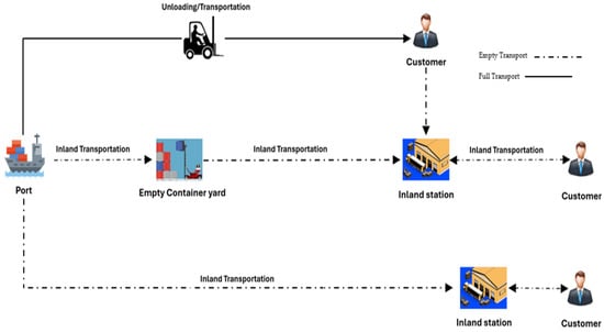
Figure 1.
Inland empty container flow in a two-depot service, adapted from [52].
Trucks are commonly used for short-haul movements due to their flexibility, while rail is preferred for longer distances because of its higher capacity and lower emissions per container-kilometer. Once containers are unloaded at customer locations, they are returned empty to nearby inland depots or back to the port, completing the cycle. This system, however, involves a significant number of empty container movements, particularly across inland routes. These empty trips contribute to operational inefficiencies and increased greenhouse gas (GHG) emissions, especially when road transport is used.
Building on the container flow illustrated in the previous figure, further operational details reveal how storage policies, repositioning needs, and customer distribution patterns shape the inland handling of empty containers. To avoid such additional storage costs and customs complexity inside the port, all empty containers are pulled out by any inland transportation modes to the inland freight station. All the empty containers stay idle in the inland station waiting to receive a customer’s request. In general, the customers are not located directly near the inland depot; therefore, shipping companies must arrange for the transportation of empty containers directly to the customer’s location within the hinterland. This means that repositioning of empty containers should be conducted between depots to restore balance in the distribution of containers across the entire service network, in alignment with transportation demand. Hence, when the shipping line receives a booking request from the customer, it moves empty containers to be transported to their premises by inland transportation.
All these additional land movements of empty containers, both within and beyond port areas, contribute significantly to environmental degradation and congestion at local and regional levels. Therefore, shipping companies prioritize the management and optimization of a physical network comprising inland depots, ports, and customer locations. This strategy focuses on minimizing unnecessary empty container movements, thereby enhancing efficiency and mitigating environmental impacts.
4. ABM Formulation
Traditional optimization approaches such as mixed-integer programming (MIP) and VRP have been widely used in maritime transportation to solve route planning, fleet deployment, and scheduling problems. They typically rely on centralized decision-making, fixed inputs, and deterministic rules, which may not adequately capture the complex, decentralized, and dynamic nature of real-world maritime logistics problems. In contrast, ABM provides a flexible and bottom-up approach that enables the modeling of heterogeneous agents such as shipping lines, ports, terminals, vehicles, and containers, with autonomous behaviours and localized decision-making processes [53].
ABM is particularly well suited for scenarios where system-level patterns emerge from individual interactions, rather than being dictated by a central planner. Moreover, ABM allows for easy scenario testing under various operational and behavioral assumptions, supporting experimentation with adaptive strategies and policy interventions [54]. This is in contrast to optimization models, which often require reformulation and resolving when system parameters or objectives change.
This methodological flexibility makes ABM not only a modeling tool but also an exploratory platform to understand the resilience and adaptability of container transportation systems under uncertainty. Therefore, the use of ABM in this paper is not simply a matter of preference but a deliberate choice to better reflect the real-world characteristics of empty container movements. ABM provides a complementary and, in many cases, more realistic alternative to traditional optimization approaches, especially in environments characterized by high uncertainty, heterogeneity, and adaptive behavior [55]. Hence, it is a powerful tool for simulating and optimizing the movement of empty containers within two-depot systems. By modeling these agents and their behaviours, ABM can provide insights into waiting time, container availability, and CO2 emissions.
In the model, CO2 emissions can be calculated with the CarbonCare CO2 calculator for each move of inland transportation, which estimates emissions based on road distance, truck type, and load factors. This calculator uses the European EN 16258 standard [44]. The calculations were based on the tare weight of an empty twenty-foot equivalent unit (TEU), which is approximately 2300 km [56], and the vehicle type is a 40-tonne truck. The total emissions are calculated by multiplying the number of vehicles by the distance travelled and the emission factor, using the following formula:
Emissions = ∑ (Number of vehicles × Distance × Emission Factor)
JADE, NetLogo, AnyLogic, StarLogo, and RePast are the most frequently mentioned agent-based platforms for supply chain problems. These platforms can be used to track the actions of all supply chain participants throughout time, as well as the supply chain overall. They allow decision-makers to simulate multiple “what-if” scenarios involving container repositioning. They can simulate the effect of using different transport modes, optimizing container routes, or adjusting scheduling to reduce emissions. Furthermore, the NetLogo 6.2.2 simulation platform, which is designed to model complex systems using visual shapes and graphs, was chosen in this study. Agents are expressed in the form of turtles, patches, links, and the observer [57]. NetLogo simulates intricate social and ecological systems. Its user-friendly platform allows it to be applied to complex interactions between numerous stakeholders when it is difficult to characterize their patterns of behavior. Numerous scientific fields, including computer science, resource management, and decision-making, have used NetLogo programming.
4.1. Model Assumptions
The model is tailored for the repositioning of empty containers in the hinterland in the representative setting of a network of empty container yards, inland freight stations, and customer locations. To simplify the problem formulation, the assumptions should be clearly defined, all of which are commonly found in the literature.
Assumption 1: A closed system, consisting of only four nodes: ports, container yards, inland freight stations, and customer locations. As such, empty containers can only be transported or repositioned between these four nodes, and containers outside the system are not permitted to enter.
Assumption 2: Well-performing containers: containers are assumed to be in good condition, meaning that container maintenance is not addressed within the scope of the problem.
Assumption 3: Transportation modes: trucks are considered the primary mode of transportation for inland container movement in the model.
Assumption 4: Intermediary property of depots: it is assumed that full containers are discharged at customer locations and subsequently returned to empty yards within the port for short-term storage, where they are kept available for future export demands. If the demand for empty containers is not yet determined, they will be moved to an inland freight station for long-term storage, awaiting customer requests.
Assumption 5: Single transport cost: it is assumed there only exists one transport cost between each pair of demand and supply, that is, deterministic transportation costs between two specific locations.
Assumption 6: Storage costs: it is assumed that the cost of storing containers in the empty yard and freight station is negligible or not a primary factor in environmental analysis. This exclusion allows the model to focus on the structural and environmental impacts of inland container movements without introducing cost variability, which can differ significantly across regions and operators.
Assumption 7: Capacity: the capacity of the empty container yard and inland station depots for storing containers is infinite.
Assumption 8: Type of container: only standard containers, whether 20- or 40-foot containers, are employed for transportation. Special equipment is not considered as it needs to be moved by specific instructions.
4.2. Entities and State Variables
The following tables outline key entities and state variables in the NetLogo simulation model, including trucks, depots, ports, customers, and links. In Table 1, each entity is defined by specific attributes that govern its role. Additionally, the core sets representing agents and network elements are listed in Table 2, while the associated system parameters relevant to container flows, demand, and emissions are detailed in Table 3.

Table 1.
Agents.
Table 2.
Sets.
Table 3.
Parameters.
Table 1 shows several types of agents that represent the key components of the simulation model. The port agent type signifies the main location represented in Jeddah Islamic Port where trucks load and unload containers. The truck agent type represents the vehicles transporting 20-foot containers, each with parameters like (indicating whether the truck is carrying a load), (the current target location), and (the route to follow). Depots are agents that hold storage capacity for containers and current storage levels, facilitating the management of container inventory. The first depot is Red Sea Gateway Terminal (RSGT) and the second one is Mansour Al Otaibi & Partners Group (OHT). Customers represent various client locations, characterized by parameters such as , which tracks the number of containers needed, and , determining how often they request shipments. Lastly, nodes act as intermediate points on the truck routes, helping to define the geographical structure of the road network. The model’s global parameters, including total emission and time-tracking variables (current-minute, current-hour, current-day, and current-year), support the simulation by providing essential data on emissions and the progression of time within the model. Together, these agents and parameters create a comprehensive framework for simulating and analyzing the movement of empty containers within two-depot systems and transport efficiency in the specified region.
4.3. Mathematical Model for Empty Container Movements
To provide a clearer representation of the NetLogo model within the movement of empty containers within two depot-systems, a mathematical formulation is introduced in this section. First, in Table 4 the decision variables representing the truck movements, container deliveries, and storage states are defined to capture the operational dynamics of the system. Then, the objective function to minimize total CO2 emissions from truck movements between the depots over the time horizon is formulated, followed by constraints that ensure the operational feasibility of the solution.
Table 4.
Decision variables.
Objective Function:
Constraints:
Truck Flow Conservation: For each truck , node , and time period , ensure that a truck entering a node must leave it (or remain idle):
Truck Availability: Each truck can only travel one route at a time:
Customer Demand Satisfaction: The number of containers delivered to customer in time period plus unmet demand must meet or exceed the demand:
Container Delivery: Containers delivered to customers come from loaded trucks arriving at the customer node:
Depot Storage Balance: For each depot , the number of stored containers is updated based on incoming and outgoing containers:
Depot Capacity: Storage at depots cannot exceed capacity:
Port as Container Source: Containers originate from the port (JIP) when trucks leave with loaded containers:
Non-negativity and binary constraints:
4.4. Model Procedures
The NetLogo model follows a structured sequence: initialization and execution. Below is a detailed breakdown of each phase:
Step 1: Model Initialization
The model uses GIS shapefile and CSV as inputs to generate the port, empty yard, inland terminal, and customer premises. The model simulates the movement of empty 20 ft containers using 40 ft trucks in a two-depot system within Jeddah, Saudi Arabia. Figure 2 shows the interface of the build model; the GIS-based map on the left visualizes the road network, with truck movements. The color-coded symbols indicate ports (red star), empty container depots (red squares), and inland depots (green dots). The model uses four plots monitoring CO2 emission of empty truck movements, container status, waiting time of customers, and unmet demand. The GHG emission plot measures the increase in CO2 emissions over time based on real-world fuel consumption, which may require optimization. The truck container status plot exhibits a cyclical pattern, indicating that trucks continuously switch between loaded and unloaded states, reflecting a hub-and-spoke logistics system. Additionally, the customer waiting time and the unfilled demand plot also show if a customer faces a delay in receiving their containers, or if the demand is not being met. To enhance the efficiency of the model, several sliders/switches are added to adjust the actions taken by the agents, whether at the start-up process or during run-time.
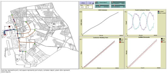
Figure 2.
The NetLogo interface of truck movements for empty containers.
Step 2: Run
Once initialized, the model is run using the GO button. When the model begins, the truck with an empty container moves to an empty depot in the port to be stored until it is released. Then, empty containers are pulled out by inland transportation to the inland terminal waiting for their demand, heading to the customer. By clicking on the OFF button for the inland depot, the truck will head to the customer location, which affects the four plots, namely, time, cost, demand, and emission. The simulated time progresses in minutes, with ticks representing 1 min. Additionally, the model runs for 5 simulated years. The results for both routes are visualized in plots over time based on load status by repeating until 5 simulated years elapse.
4.5. Expermintal Design
To assess the performance of the proposed ABM and highlight its added value, a baseline scenario was developed to emulate current empty movement practices within two-depot systems. A baseline scenario was implemented within the same agent-based framework to reflect the same logistics operations in empty container movements. This scenario replicates centralized, rule-based logistics practices, in contrast to the decentralized and adaptive behavior of the full ABM configuration. Truck agents operate with static shortest path routing and dispatch only when a container request is received, without anticipatory routing or emissions considerations. Depots function independently, replenishing stock at fixed intervals, and fulfilling customer requests on a First-In, First-Out (FIFO) basis. No dynamic reallocation of stock or coordination between depots is performed. Customers submit periodic container requests and remain passive until fulfilment. Ports operate with static schedules and serve agents in arrival order. Links are treated equally regardless of time or usage.
A baseline scenario representing current logistics practices was constructed based on prevailing logistics practices, particularly the use of direct truck routing without intermediary depots [58]. Moreover, its outcomes match anticipated trends in systems lacking depot coordination, supporting its credibility for meaningful comparison with the proposed ABM scenario [59,60]. Key performance metrics, such as delivery times, unmet requests, CO2 emissions, and depot utilization, are used to assess the improvements enabled by the proposed model. Furthermore, the NetLogo model uses Behavior Space to conduct sensitivity analysis by varying the following parameters and testing a serial variable by varying parameters and recording outputs. The experimental design focuses on analyzing the effect of empty container truck movements under two different scenarios: Scenario A (baseline without inland depots) and Scenario B (proposed ABM with inland depots) under the same input conditions. The baseline scenario was constructed to emulate existing centralized practices, where empty containers are delivered directly without intermediate depot coordination or environmental optimization, common in regional container transport systems such as those in the Gulf and East Africa [61].
Table 5 explains the main two key parameters that varied in the experiment. The first one determines whether empty containers are first stored in inland depots before being transported to customers or if they are delivered directly to customer locations. The second one explores the impact of different demand intervals, simulating how varying container request frequencies affect movement performance. Hence, Behavior Space can provide insights for decision-making in reducing emissions and improving transport efficiency.
Table 5.
Parameter variations in sensitivity analysis.
As shown in Table 6, the model tracks several key metrics to evaluate performance. Total emission measures total CO2 emissions in kilograms, reflecting environmental impact, the counts of trucks actively transporting containers, the idle or empty trucks, which contribute to inefficiencies, the average waiting time for customers before receiving their containers, and the average unmet demand per customer.
Table 6.
Output metrics.
5. Results and Discussion
The sensitivity analysis conducted via Behavior Space confirmed the robustness of these trends across a range of demand frequencies and routing strategies. By comparing the two operational scenarios with inland depot coordination (inland-depot? = true) and without depot usage (inland-depot? = false), the simulation highlights key differences in system efficiency, emissions, and service quality. The results show that container availability, customer waiting time, and CO2 emissions are highly related to the customer demand frequency. Subsequently, Figure 3 shows the variation in the number of empty containers over time (in days) based on different demand frequency levels (from 1 to 6) within the model.
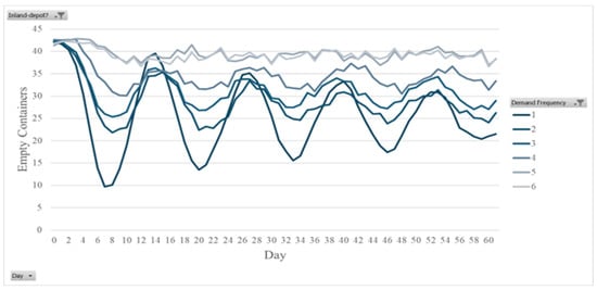
Figure 3.
Customer demand frequency levels.
To maintain fair comparisons across two different scenarios, a demand frequency of 3 days is chosen as a baseline for further analysis. The selection of a 3-day customer demand frequency is grounded in a balance between system stability and analytical clarity. Through simulation, it was observed that shorter demand intervals (such as 1 or 2 days) led to higher system stress, characterized by sharp fluctuations in empty container availability and increased CO2 emissions due to frequent movements. Conversely, longer intervals (such as 5 or 6 days) resulted in underutilization of resources and stagnant system dynamics, where container flows and emissions remained relatively flat and less informative for analysis. Moreover, the selected demand frequency of 3 days as an optimal point can produce enough activity to highlight inefficiencies and potential improvements while keeping the system within operational realism. These findings validate the model’s capacity to support logistics decision-making under dynamic, real-world conditions and demonstrate its added value over conventional practices.
Figure 4 illustrates the cumulative GHG emissions in tons over time under two different scenarios. Both scenarios show steadily increasing total GHG emissions over time, following a nearly linear growth pattern. When inland depots are used, which is represented by the orange line, emissions increase at a slightly lower rate, resulting in approximately 1000–1500 tons less CO2 emissions compared to the direct routing system. This scenario can reduce the total CO2 emissions by approximately 15–25% compared to direct customer routing. This is due to the better consolidation of container movements, reducing unnecessary trips. However, if trucks move directly to customer locations without utilizing the depot, emissions accumulate at a faster rate, resulting in a 20–30% increase in emissions due to increased trips and empty backhauls.
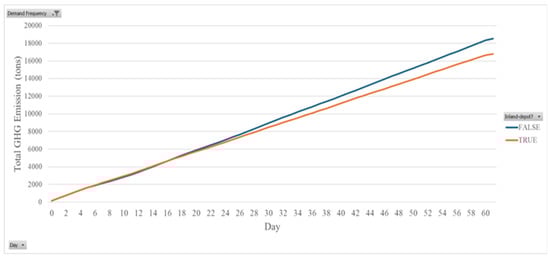
Figure 4.
GHG emissions under different scenarios.
Figure 5 demonstrates the number of empty containers over time under two different scenarios. When the inland depot is utilized, the number of empty containers stabilizes at a consistently lower level. The inland depot functions as a buffer, allowing for better coordination and redistribution of empty containers, which reduces the peaks and troughs seen in the other scenario. It leads to a reduction in empty container accumulation, implying that containers are being utilized more efficiently rather than sitting idle in depots or ports. This indicates a more balanced and efficient system where empty containers are allocated in a way that aligns better with demand patterns, whereas the number of empty containers in the direct strategy exhibits more pronounced fluctuations, with sharp drops and recoveries throughout the simulated period. This suggests inefficiencies in container circulation can be addressed to reduce bottlenecks in the supply chain.
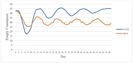
Figure 5.
The availability of empty containers.
Figure 6 measures the average customer waiting time over the simulation period for both scenarios. The relationship between customer waiting time, unmet demand levels, and the configuration of the inland depot is very significant. Moreover, the results show that when an inland depot is used, customer waiting time increases exponentially, suggesting severe delays. Conversely, without an inland depot, waiting times remain stable. This means that direct routing ensures a more efficient and responsive supply chain, with containers reaching their destinations in a timely manner. However, it may lead to higher unmet demand if trucks are not available when needed. Meanwhile, the result shows that while the inland depot system may be beneficial in terms of environmental impact and overall container efficiency, it comes at the cost of severely reduced service levels for customers.
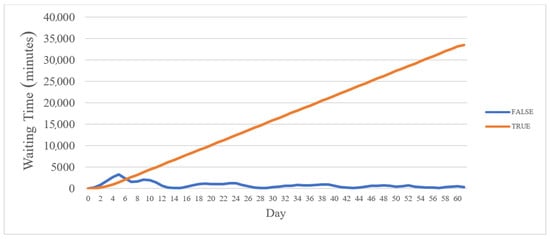
Figure 6.
The average waiting time under different scenarios.
The sensitivity analysis using Behavior Space revealed that customer demand frequency and depot routing significantly influence emissions and waiting time. The proposed ABM consistently outperformed the baseline in all tested configurations, indicating robust performance under varying operational conditions. Hence, the statistical evidence highlights that the depot system significantly reduces emissions and optimizes truck utilization, but it increases the average waiting times due to additional storage processes. By comparison, the direct routing scenario is advantageous in minimizing delivery delays but results in higher emissions and operational costs. Hence, this result highlights a major trade-off between cost, time, and sustainability. Ultimately, the model suggests that while an inland depot enhances sustainability and logistical efficiency, it does so at the expense of customer satisfaction. Decision-makers must balance these factors based on operational priorities, and whether they prioritize environmental benefits and cost reductions or faster service and system flexibility.
6. Conclusions and Future Research
In this study, we investigated the importance of managing inland movements of empty containers in modern logistics and supply chain operations. This paper proposes a simulation optimization model for the movements of empty containers among a two-depot system and their impact on CO2 emissions, customer waiting times, and system efficiency. ABM successfully captures real-world complexities to simulate the truck movements between the port, inland depots, and customer premises. In this way, the analysis highlights the significant influence of demand frequency and inland depot utilization on network performance. The findings provide several practical implications for logistics managers and policymakers engaged in maritime container transport. According to the simulation, using inland depots can cut greenhouse gas emissions by around 15–25% and help create more stable and effective container circulation by reducing the accumulation of empty containers. These results suggest that inland depots can serve as effective coordination hubs, particularly in heavy-traffic regions or where environmental sustainability is a priority. However, the results also reveal a trade-off between environmental benefits and service efficiency: while depot-based routing supports emission reduction, it may also lead to increased customer waiting times due to added handling activities and longer distances.
To address this, decision-makers may consider adopting hybrid routing strategies, where urgent or time-sensitive deliveries follow direct routes, while others are routed through depots to optimize consolidation. Moreover, the reduced variability in empty container flows under the depot scenario highlights the potential of shared depots or container pooling systems to improve equipment utilization and lower operational costs. In practice, companies like Maersk and Hapag-Lloyd are already experimenting with differentiated delivery options and dynamic dispatching technologies to optimize fleet utilization without compromising customer responsiveness. These hybrid strategies, wherein time-sensitive deliveries are routed directly while bulk or lower-priority shipments utilize depot infrastructure, mirror the adaptive approach proposed by this study. From an operational planning perspective, this study demonstrates the value of agent-based modeling as a decision support tool. It enables managers to evaluate different logistics strategies under variable demand and operational constraints before implementation, thereby reducing risk. Furthermore, the model offers a framework for policymakers to assess the impact of routing configurations on emissions, providing a basis for formulating incentives or regulations that encourage more sustainable logistics practices.
The proposed ABM was developed to explore the environmental impact of inland empty container movements within a two-depot system. To maintain simplicity, the model includes assumptions such as a closed system, ideal container conditions, and unlimited depot storage. While these help clarify the model’s focus, they limit its ability to fully reflect real-world logistics complexities. Additionally, the use of NetLogo as a modeling platform further supports agent-based logic and visualization but presents limitations in terms of computational scalability and performance for large-scale applications.
Nevertheless, while ABM is a powerful tool for analyzing complex logistics systems, it has certain limitations. These include high computational requirements for large-scale simulations, reliance on detailed behavioral data, and a lack of standardized frameworks, which can affect model consistency and comparability. Additionally, interpreting emergent behaviours can be challenging without support from complementary analytical methods. Recognizing these constraints, future research should focus on leveraging high-performance computing, integrating real-time and empirical data, and developing standardized modeling practices. Hybrid approaches that combine ABM with optimization or system dynamics could also enhance model transparency and decision-making utility. The modular structure of the ABM also allows future extensions to integrate economic metrics for more comprehensive trade-off analysis. Hence, an important extension of the current model will be to incorporate detailed cost metrics alongside environmental performance.
Beyond methodological improvements, there are several avenues to extend the practical relevance of this framework. While the current model offers valuable insights into emission reduction and container flow optimization, it simplifies certain operational realities. Future enhancements could incorporate dynamic pricing strategies, network congestion effects, and stochastic demand patterns to enable comprehensive trade-off analyses between economic performance, service levels, and environmental impact. Additionally, evaluating the adoption of sustainable transport technologies, such as electric or hydrogen-powered trucks, could further advance emissions reduction goals while maintaining logistical efficiency. Finally, coupling maritime container repositioning models with detailed inland transport simulations would provide a more holistic view of empty container flows across multimodal networks, thereby enhancing the model’s applicability to real-world logistics challenges.
Author Contributions
Conceptualization, A.A. and T.K.; Methodology, A.A. and T.K.; Software, A.A.; Validation; T.K.; Writing—original draft preparation, A.A. and M.S.; Writing—review and editing, A.A. and M.S.; supervision, T.K. All authors have read and agreed to the published version of the manuscript.
Funding
This research received no external funding.
Institutional Review Board Statement
Not applicable.
Informed Consent Statement
Not applicable.
Data Availability Statement
Data are contained within the article.
Conflicts of Interest
The authors declare no conflicts of interest.
References
- UNCTAD. Review of maritime transport 2018. In UNCTAD/RMT/2019; UNCTAD: Genève, Switzerland, 2019. [Google Scholar]
- Song, D.-P.; Dong, J.-X. Empty container repositioning. In Handbook of Ocean Container Transport Logistics; Springer: Berlin/Heidelberg, Germany, 2015; pp. 163–208. [Google Scholar]
- Song, D.-P.; Carter, J. Empty container repositioning in liner shipping. Marit. Policy Manag. 2009, 36, 291–307. [Google Scholar] [CrossRef]
- Abdelshafie, A.; Salah, M.; Kramberger, T.; Dragan, D. Repositioning and Optimal Re-Allocation of Empty Containers: A Review of Methods, Models, and Applications. Sustainability 2022, 14, 6655. [Google Scholar] [CrossRef]
- Xiang, X.; Liu, C.; Jia, S. Tactical vessel deployment and empty container repositioning considering container turnover times. Comput. Ind. Eng. 2024, 190, 110032. [Google Scholar] [CrossRef]
- Joung, T.-H.; Kang, S.-G.; Lee, J.-K.; Ahn, J. The IMO initial strategy for reducing Greenhouse Gas (GHG) emissions, and its follow-up actions towards 2050. J. Int. Marit. Saf. Environ. Aff. Shipp. 2020, 4, 1–7. [Google Scholar] [CrossRef]
- Moon, I.-K.; Do Ngoc, A.-D.; Hur, Y.-S. Positioning empty containers among multiple ports with leasing and purchasing considerations. OR Spectr. 2010, 32, 765–786. [Google Scholar] [CrossRef]
- Hu, H.; Du, B.; Bernardo, M. Leasing or repositioning empty containers? Determining the time-varying guide leasing prices for decision making. Marit. Policy Manag. 2021, 48, 829–845. [Google Scholar] [CrossRef]
- Song, J.; Tang, X.; Wang, C.; Xu, C.; Wei, J. Optimization of multi-port empty container repositioning under uncertain environments. Sustainability 2022, 14, 13255. [Google Scholar] [CrossRef]
- Namboothiri, R.; Erera, A.L. Planning local container drayage operations given a port access appointment system. Transp. Res. Part E Logist. Transp. Rev. 2008, 44, 185–202. [Google Scholar] [CrossRef]
- Hassanin, I.; Serra, P.; Iskander, J.; Gamboa-Zamora, S.; Knez, M. Is the inland waterways system primed for mitigating road transport in Egypt? Int. Bus. Logist. 2024, 4, 61–77. [Google Scholar] [CrossRef]
- Ongcunaruk, W.; Ongkunaruk, P.; Janssens, G. Time Window Characteristics in a Heuristic Algorithm for a Full-Truck Vehicle Routing Heuristic Algorithm in An Intermodal Context. J. Optimasi Sist. Ind. 2025, 24, 18–36. [Google Scholar] [CrossRef]
- Huang, Y.; Jin, Z.; Liu, P.; Wang, W.; Zhang, D. Container drayage problem integrated with truck appointment system and separation mode. Comput. Ind. Eng. 2024, 193, 110307. [Google Scholar] [CrossRef]
- Song, D.-P.; Earl, C.F. Optimal empty vehicle repositioning and fleet-sizing for two-depot service systems. Eur. J. Oper. Res. 2008, 185, 760–777. [Google Scholar] [CrossRef]
- Lu, T.; Lee, C.-Y.; Lee, L.-H. Coordinating pricing and empty container repositioning in two-depot shipping systems. Transp. Sci. 2020, 54, 1697–1713. [Google Scholar] [CrossRef]
- Blažina, A.; Ivče, R.; Mohović, Đ.; Mohović, R. Analysis of empty container management. Pomor. Sci. J. Marit. Res. 2022, 36, 305–317. [Google Scholar] [CrossRef]
- Olivo, A.; Di Francesco, M.; Zuddas, P. An optimization model for the inland repositioning of empty containers. In Port Management; Springer: Berlin/Heidelberg, Germany, 2015; pp. 84–108. [Google Scholar]
- Notteboom, T.; Pallis, A.; Rodrigue, J.-P. Port Economics, Management and Policy; Routledge: London, UK, 2022. [Google Scholar]
- Yu, X.; Feng, Y.; He, C.; Liu, C. Modeling and Optimization of Container Drayage Problem with Empty Container Constraints across Multiple Inland Depots. Sustainability 2024, 16, 5090. [Google Scholar] [CrossRef]
- Dang, Q.-V.; Nielsen, I.E.; Yun, W.-Y. Replenishment policies for empty containers in an inland multi-depot system. Marit. Econ. Logist. 2013, 15, 120–149. [Google Scholar] [CrossRef]
- Helo, P.; Rouzafzoon, J. An agent-based simulation and logistics optimization model for managing uncertain demand in forest supply chains. Supply Chain. Anal. 2023, 4, 100042. [Google Scholar] [CrossRef]
- Calabrò, G.; Le Pira, M.; Giuffrida, N.; Fazio, M.; Inturri, G.; Ignaccolo, M. Modelling the dynamics of fragmented vs. consolidated last-mile e-commerce deliveries via an agent-based model. Transp. Res. Procedia 2022, 62, 155–162. [Google Scholar] [CrossRef]
- Larrea-Gallegos, G.; Benetto, E.; Marvuglia, A.; Gutiérrez, T.N. Sustainability, resilience and complexity in supply networks: A literature review and a proposal for an integrated agent-based approach. Sustain. Prod. Consum. 2022, 30, 946–961. [Google Scholar] [CrossRef]
- Dejax, P.J.; Crainic, T.G. Survey Paper—A Review of Empty Flows and Fleet Management Models in Freight Transportation. Transp. Sci. 1987, 21, 227–248. [Google Scholar] [CrossRef]
- Crainic, T.G.; Dejax, P.; Delorme, L. Models for multimode multicommodity location problems with interdepot balancing requirements. Ann. Oper. Res. 1989, 18, 277–302. [Google Scholar] [CrossRef]
- Crainic, T.G.; Gendreau, M.; Dejax, P. Dynamic and stochastic models for the allocation of empty containers. Oper. Res. 1993, 41, 102–126. [Google Scholar] [CrossRef]
- Holmberg, K.; Joborn, M.; Lundgren, J.T. Improved empty freight car distribution. Transp. Sci. 1998, 32, 163–173. [Google Scholar] [CrossRef]
- Choong, S.T.; Cole, M.H.; Kutanoglu, E. Empty container management for intermodal transportation networks. Transp. Res. Part E Logist. Transp. Rev. 2002, 38, 423–438. [Google Scholar] [CrossRef]
- Arnold, P.; Peeters, D.; Thomas, I. Modelling a rail/road intermodal transportation system. Transp. Res. Part E Logist. Transp. Rev. 2004, 40, 255–270. [Google Scholar] [CrossRef]
- Erera, A.L.; Morales, J.C.; Savelsbergh, M. Global intermodal tank container management for the chemical industry. Transp. Res. Part E Logist. Transp. Rev. 2005, 41, 551–566. [Google Scholar] [CrossRef]
- Olivo, A.; Zuddas, P.; Di Francesco, M.; Manca, A. An operational model for empty container management. Marit. Econ. Logist. 2005, 7, 199–222. [Google Scholar] [CrossRef]
- Bin, W.; Zhongchen, W. Research on the optimization of intermodal empty container reposition of land-carriage. J. Transp. Syst. Eng. Inf. Technol. 2007, 7, 29–33. [Google Scholar]
- Boile, M.; Theofanis, S.; Baveja, A.; Mittal, N. Regional repositioning of empty containers: Case for inland depots. Transp. Res. Rec. 2008, 2066, 31–40. [Google Scholar] [CrossRef]
- Zhang, R.; Yun, W.Y.; Kopfer, H. Heuristic-based truck scheduling for inland container transportation. OR Spectr. 2010, 32, 787–808. [Google Scholar] [CrossRef]
- Yao, B.; Yu, B.; Hu, P.; Gao, J.; Zhang, M. An improved particle swarm optimization for carton heterogeneous vehicle routing problem with a collection depot. Ann. Oper. Res. 2016, 242, 303–320. [Google Scholar] [CrossRef]
- Peng, Z.; Wang, H.; Wang, W.; Jiang, Y. Intermodal transportation of full and empty containers in harbor-inland regions based on revenue management. Eur. Transp. Res. Rev. 2019, 11, 7. [Google Scholar] [CrossRef]
- Faber, J.; Hanayama, S.; Zhang, S.; Pereda, P.; Comer, B.; Hauerhof, E.; Schim van der Loeff, W.; Smith, T.; Zhang, Y.; Kosaka, H. Fourth IMO greenhouse gas study. Int. Marit. Organ. 2020, 5, 2022. [Google Scholar]
- UNCTAD. Bold global action needed to decarbonize shipping and ensure just transition. In UNCTAD Report; UNCTAD: Genève, Switzerland, 2023. [Google Scholar]
- Englert, B.; Lam, S.; Steinhoff, P. The Impact of Truck Repositioning on Congestion and Pollution in the LA Basin. 2011. Available online: https://rosap.ntl.bts.gov/view/dot/23264 (accessed on 20 August 2024).
- Schulte, F.; González, R.G.; Voß, S. Reducing port-related truck emissions: Coordinated truck appointments to reduce empty truck trips. In Proceedings of the Computational Logistics: 6th International Conference, ICCL 2015, Delft, The Netherlands, 23–25 September 2015; pp. 495–509. [Google Scholar]
- Schulte, F.; Lalla-Ruiz, E.; González-Ramírez, R.G.; Voß, S. Reducing port-related empty truck emissions: A mathematical approach for truck appointments with collaboration. Transp. Res. Part E Logist. Transp. Rev. 2017, 105, 195–212. [Google Scholar] [CrossRef]
- Bektaş, T.; Laporte, G. The pollution-routing problem. Transp. Res. Part B Methodol. 2011, 45, 1232–1250. [Google Scholar] [CrossRef]
- Sporkmann, J.; Liu, Y.; Spinler, S. Carbon emissions from European land transportation: A comprehensive analysis. Transp. Res. Part D Transp. Environ. 2023, 121, 103851. [Google Scholar] [CrossRef]
- Saharidis, G.K.; Konstantzos, G.E. Critical overview of emission calculation models in order to evaluate their potential use in estimation of Greenhouse Gas emissions from in port truck operations. J. Clean. Prod. 2018, 185, 1024–1031. [Google Scholar] [CrossRef]
- Duan, L.; Hu, W.; Deng, D.; Fang, W.; Xiong, M.; Lu, P.; Li, Z.; Zhai, C. Impacts of reducing air pollutants and CO2 emissions in urban road transport through 2035 in Chongqing, China. Environ. Sci. Ecotechnol. 2021, 8, 100125. [Google Scholar] [CrossRef]
- Kazancoglu, Y.; Ozbiltekin-Pala, M.; Ozkan-Ozen, Y.D. Prediction and evaluation of greenhouse gas emissions for sustainable road transport within Europe. Sustain. Cities Soc. 2021, 70, 102924. [Google Scholar] [CrossRef]
- Osama, A.; Bagwari, A.; Hossam, N. The Effect of Using Intelligent Transportation Systems on Transportation-Sustainable Development in Egypt. In Cases on International Business Logistics in the Middle East; IGI Global: Hershey, PA, USA, 2023; pp. 73–90. [Google Scholar]
- Zhao, C.; Wang, K.; Dong, X.; Dong, K. Is smart transportation associated with reduced carbon emissions? The case of China. Energy Econ. 2022, 105, 105715. [Google Scholar] [CrossRef]
- Erdogan, S.; Sarkodie, S.A.; Adedoyin, F.F.; Bekun, F.V.; Owusu, P.A. Analyzing transport demand and environmental degradation: The case of G-7 countries. Environ. Dev. Sustain. 2024, 26, 711–734. [Google Scholar] [CrossRef]
- Griffiths, L.L.; Connolly, R.M.; Brown, C.J. Critical gaps in seagrass protection reveal the need to address multiple pressures and cumulative impacts. Ocean Coast. Manag. 2020, 183, 104946. [Google Scholar] [CrossRef]
- Shintani, K.; Konings, R.; Imai, A. Combinable containers: A container innovation to save container fleet and empty container repositioning costs. Transp. Res. Part E Logist. Transp. Rev. 2019, 130, 248–272. [Google Scholar] [CrossRef]
- Chen, K.; Lu, Q.; Xin, X.; Yang, Z.; Zhu, L.; Xu, Q. Optimization of empty container allocation for inland freight stations considering stochastic demand. Ocean Coast. Manag. 2022, 230, 106366. [Google Scholar] [CrossRef] [PubMed]
- Macal, C.M.; North, M.J. Tutorial on agent-based modeling and simulation. In Proceedings of the Winter Simulation Conference, Orlando, FL, USA, 4 December 2005; IEEE: Piscataway, NJ, USA, 2005; p. 14. [Google Scholar]
- Niazi, M.; Hussain, A. Agent-based computing from multi-agent systems to agent-based models: A visual survey. Scientometrics 2011, 89, 479–499. [Google Scholar] [CrossRef]
- Christos, K.; Dimitrios, B.; Dimitrios, A. Agent-based simulation for modeling supply chains: A comparative case study. Int. J. New Technol. Res. 2016, 2, 36–39. [Google Scholar]
- Martin, S.; Martin, J.; Lai, P. International container design regulations and ISO standards: Are they fit for purpose? Marit. Policy Manag. 2019, 46, 217–236. [Google Scholar] [CrossRef]
- Sulis, E.; Taveter, K. Agent-Based Simulation with NetLogo. In Agent-Based Business Process Simulation: A Primer with Applications and Examples; Springer: Berlin/Heidelberg, Germany, 2022; pp. 53–75. [Google Scholar]
- Emde, S.; Zehtabian, S. Scheduling direct deliveries with time windows to minimise truck fleet size and customer waiting times. Int. J. Prod. Res. 2019, 57, 1315–1330. [Google Scholar] [CrossRef]
- Veenstra, A.; de Waal, A. The impact of container call size evidence from simulation modelling. Marit. Transp. Res. 2024, 6, 100109. [Google Scholar] [CrossRef]
- Danladi, C.; Tuck, S.; Tziogkidis, P.; Tang, L.; Okorie, C. Efficiency analysis and benchmarking of container ports operating in lower-middle-income countries: A DEA approach. J. Shipp. Trade 2024, 9, 7. [Google Scholar] [CrossRef]
- Kipyegon, N. Inter-Organizations Technology Systems’ Data Analytics, Corridor Performance Monitoring Using the Northern Transport Corridor Observatory. Doctoral dissertation, University of Nairobi, Nairobi, Kenya, 2018. [Google Scholar]
Disclaimer/Publisher’s Note: The statements, opinions and data contained in all publications are solely those of the individual author(s) and contributor(s) and not of MDPI and/or the editor(s). MDPI and/or the editor(s) disclaim responsibility for any injury to people or property resulting from any ideas, methods, instructions or products referred to in the content. |
© 2025 by the authors. Licensee MDPI, Basel, Switzerland. This article is an open access article distributed under the terms and conditions of the Creative Commons Attribution (CC BY) license (https://creativecommons.org/licenses/by/4.0/).